Industrial and Manufacturing Systems Engineering
Publications
Industrial and Manufacturing Systems Engineering
7-29-2019
Identifying and mitigating supply chain risks using
fault tree optimization
Michael D. Sherwin
Mississippi State University
Hugh R. Medal
University of Tennessee, Knoxville
Cameron A. MacKenzie
Iowa State University, [email protected]
Kennedy J. Brown
Mississippi State University
Follow this and additional works at:
https://lib.dr.iastate.edu/imse_pubs
Part of the
Operational Research Commons
, and the
Systems Engineering Commons
The complete bibliographic information for this item can be found at
https://lib.dr.iastate.edu/
imse_pubs/207
. For information on how to cite this item, please visit
http://lib.dr.iastate.edu/
howtocite.html
.
This Article is brought to you for free and open access by the Industrial and Manufacturing Systems Engineering at Iowa State University Digital Repository. It has been accepted for inclusion in Industrial and Manufacturing Systems Engineering Publications by an authorized administrator of Iowa State University Digital Repository. For more information, please [email protected].
Identifying and mitigating supply chain risks using fault tree optimization
Abstract
Although supply chain risk management and supply chain reliability are topics that have been studied extensively, a gap exists for solutions that take a systems approach to quantitative risk mitigation decision making and especially in industries that present unique risks. In practice, supply chain risk mitigation decisions are made in silos and are reactionary. In this article, we address these gaps by representing a supply chain as a system using a fault tree based on the bill of materials of the product being sourced. Viewing the supply chain as a system provides the basis to develop an approach that considers all suppliers within the supply chain as a portfolio of potential risks to be managed. Next, we propose a set of mathematical models to proactively and quantitatively identify and mitigate at-risk suppliers using enterprise available data with consideration for a firm’s budgetary constraints. Two approaches are investigated and demonstrated on actual problems experienced in industry. The examples presented focus on Low-Volume High-Value (LVHV) supply chains that are characterized by long lead times and a limited number of capable suppliers, which make them especially susceptible to disruption events that may cause delays in delivered products and subsequently increase the financial risk exposure of the firm. Although LVHV supply chains are used to demonstrate the methodology, the approach is applicable to other types of supply chains as well. Results are presented as a Pareto frontier and demonstrate the practical application of the methodology.
Keywords
Supply chain management, risk, optimization, fault tree
Disciplines
Operational Research | Systems Engineering
Comments
This is an Accepted Manuscript of an article published by Taylor & Francis as Sherwin, Michael D., Hugh R. Medal, Cameron A. MacKenzie, and Kennedy J. Brown. "Identifying and mitigating supply chain risks using fault tree optimization."IISE Transactions(2019). DOI:10.1080/24725854.2019.1630865. Posted with permission.
Identifying and mitigating supply chain risks using fault
1
tree optimization
2
Michael D. Sherwin, Hugh R. Medal, Cameron A. MacKenzie, Kennedy J. Brown
3
1 May 2019 4
Abstract
5
Although supply chain risk management and supply chain reliability are topics that have been 6
studied extensively, a gap exists for solutions that take a systems approach to quantitative risk 7
mitigation decision making and especially in industries that present unique risks. In practice, 8
supply chain risk mitigation decisions are made in silos and are reactionary. In this paper, 9
we address these gaps by representing a supply chain as a system using a fault tree based 10
on the bill of materials of the product being sourced. Viewing the supply chain as a system 11
provides the basis to develop an approach that considers all suppliers within the supply chain as 12
a portfolio of potential risks to be managed. Next, we propose a set of mathematical models to 13
proactively and quantitatively identify and mitigate at-risk suppliers using enterprise available 14
data with consideration for a firm’s budgetary constraints. Two approaches are investigated 15
and demonstrated on actual problems experienced in industry. The examples presented focus 16
on low volume high value (LVHV) supply chains that are characterized by long lead times and 17
a limited number of capable suppliers, which make them especially susceptible to disruption 18
events that may cause delays in delivered products and subsequently increase the financial risk 19
exposure of the firm. Although LVHV supply chains are used to demonstrate the methodology, 20
the approach is applicable to other types of supply chains as well. Results are presented as a 21
Pareto frontier and demonstrate the practical application of the methodology. 22
Keywords: Supply chain management, risk, optimization, fault tree
23
1
Introduction
24
In this paper, we propose a methodology to optimize the reliability of a supply chain using a fault tree
25
based on the bill of materials of the product being sourced. In addiiton, the mathematical models
26
developed return a propsed mitigation strategy for the supply chain system with consideration
27
for a firm’s budgetary constraints. Although widely applicable, we focus the application of our
methodology to the nuclear power plant construction supply chain; an industry with supply chain
29
challenges. The examples used are representative of real cases from the industry.
30
Supply chain risk management (SCRM), which is already an extensively studied topic, recently
31
became a popular area of interest because supply chains are experiencing greater exposure to risk.
32
This greater risk is the result of recent changes in how businesses are being managed. Juttner et al
33
(2003) identified the following business practices that have contributed to these increased risks: (1) a
34
focus on efficiency rather than effectiveness, (2) supply chain globalization, (3) focused factories and
35
centralized distribution, (4) a trend toward outsourcing, and (5) reduction of the supply base. Many
36
industries have experienced an increase in supply chain risks due to these practices in combination
37
with the characteristics of the industries they serve. For example, the nuclear industry is highly
38
regulated, requires significant capital investment, has high regulatory barriers to entry, experiences
39
infrequent and low quantity demands, and is primarily a make-to-design industry. This results in a
40
scarcity of capable suppliers across supply chains, which leads to single and sole source situations,
41
and makes carrying inventory buffers impractical.
42
The following elements of this paper make a novel contribution to the study of supply chain
43
risk management. First, we develop two supply chain risk mitigation models to identify at-risk
44
suppliers and optimize the overall reliability of the supply chain. More specifically, we allocate
45
resources among suppliers to maximize reliability of the supply chain. Next, we apply the approaches
46
developed within this paper to demonstrate our approach and how it could be used to solve a
47
practical problem facing a relevant industry.
48
In the next section, a literature review of related work is presented followed by an overview of
49
fault tree analysis and a summary of Sherwin et al. (2016) for those readers less familiar with the
50
subject. Next, the model formulations are outlined. We then apply the models to solve a problem
51
that faces supply chain professionals within the nuclear power industry. The paper concludes with
52
a discussion of the results and recommendations for future work.
53
2
Literature Review
54
Since the early part of the 21st century there has been a significant increase in the number of
55
published papers in the area of supply chain risk modeling (Fahimnia et al. , 2015). The SCRM
literature (Snyder, 2006; Tang et al. , 2012) contains conceptual, quantitative, and qualitative
57
methodologies applied to four primary elements of research: identification, assessment, mitigation,
58
and responsiveness (Sodhiet al. , 2012). This section presents a review of current literature in those
59
areas of research most relevant to this paper.
60
Although research focusing on supply chain risk management and related areas has increased
61
in recent years, a need remains for approaches that join both mature (e.g., tactical and operational
62
planning, demand and supply forecasting) and emergent areas (e.g., sourcing and supply uncertainty
63
modeling, sustainability risk analysis) (Qaziet al. , 2015; Fahimniaet al., 2015). Traditional
quan-64
titative operations research methodologies such as mixed integer programming (Snyder & Daskin,
65
2005; Cui et al. , 2010; Lim et al. , 2010; Benyoucef et al. , 2013; Rafiei et al. , 2013), stochastic
66
programming (Madadi et al. , 2014; Goh et al. , 2007; Bogataj et al. , 2015; Sawik, 2016; Tomlin,
67
2006; Losada et al. , 2012), fuzzy optimization (Aqlan & Lam, 2015b,a; Chen et al. , 2006a; Lee,
68
2009; Sohn & Choi, 2001), and simulation (Schmitt & Singh, 2009; Klimov & Merkuryev, 2008;
69
Wilson, 2007) have been applied to solve supply chain disruption problems quantitatively.
70
Some quantitative approaches estimate supplier risk through surveys of experienced personnel
71
(Karsak & Dursun, 2015; Aqlan & Lam, 2015b) in lieu of empirical data. Surveys, rating systems,
72
matrices, and the aggregation of data resulting from these types of methods fail to accurately
73
measure the likelihood of risks and may lead to poor management decisions (Anthony Tony Cox,
74
2008). Ivanov et al. (2015) note that it is almost impossible to determine the probability of
endemic-75
type risks such as fires, natural disasters, or piracy. Simchi-Levi et al. (2014; 2015) develop a model
76
to determine the impact of a disruption in the supply chain regardless of the cause or likelihood and
77
use a risk-exposure model to assess the impact of disruptions originating in an automotive supply
78
chain with a specific emphasis on low probability risks with high potential impact.
79
Identifying risks that can occur in a supply chain and assessing the likelihood and consequences
80
from those risks is important, but determining how best to mitigate those risks might be even more
81
important for supply chains. Strategies for mitigating disruptions include site location selection
82
(Akgünet al., 2014; Snyder & Daskin, 2005), inventory stocking levels (Tomlin, 2006; Chopraet al.
83
, 2007), and transportation decision models (MacKenzie et al. , 2012). Tomlin (2006) models a
84
firm’s ability to mitigate supply chain risk using inventory or sourcing for multiple suppliers or a
85
combination of the two. Other authors have investigated financial risk sharing within a supply chain
via contracts, pricing, or competition (Babich, 2006; Babichet al., 2007; Babich, 2010). Kleindofer
87
& Saad (2005) analyzes strategic decision making and focuses on risks arising from disruptions to
88
normal activities and the management systems to cope with such supply chain risks. Other research
89
in supply chain risk focuses on response strategies once a risk has been realized (Hishamuddinet al.
90
, 2012; Xia et al. , 2004; MacKenzieet al. , 2014).
91
Other approaches to mitigating supply chain risk concentrate on selecting less risky suppliers
92
or working with existing suppliers to mitigate risk in those suppliers’ operations. Sawik (2011)
93
proposes a portfolio approach to supplier selection with consideration for due dates, cost, and risk
94
mitigation. The author develops a mixed integer program that seeks to minimize cost and considers
95
when and from whom to purchase products based on price, quality, and supplier reliability. Chen
96
et al. (2006b) propose the use of linguistic ratings expressed as fuzzy numbers to assess both
97
qualitative and quantitative factors related to quality, price, flexibility, and delivery performance as
98
a mechanism for supplier selection. Ghodsypour & O’Brien (1998) suggest a combined analytical
99
hierarchy process and linear programming approach to consider both tangible (quantitative) and
100
intangible (qualitative) factors for choosing the optimum supplier.
101
The approach outlined in this paper can be used to select suppliers, but from the perspective
102
of the effect that supplier selection has on the supply chain system’s reliability. Like Sherwin et al.
103
(2016), we represent a supply chain as a fault tree, which provides a system view of the reliability of
104
the supply chain being studied with consideration for the overall structure of the supply chain. We
105
extend the authors’ work by developing a mixed integer program that seeks to maximize supply chain
106
reliability where each supplier has a probability of failure. The firm mitigates risk in its supply chains
107
by identifying suppliers that pose the greatest risk and then takes mitigation actions to increase the
108
reliability of those suppliers. The solution methodology to identify the optimal mitigation activities
109
converts the fault tree structure to a binary decision diagram in order to leverage the computational
110
advantages (Sinnamon & Andrews, 1997, 1996; Remenyte-Prescott & Andrews, 2007). A holistic
111
approach to proactively mitigate risks while considering multiple risk factors is another important
112
contribution of our work and has been identified as a gap in the current research (Paulet al., 2016;
113
Snyderet al. , 2016).
3
Fault Tree Analysis and Binary Decision Diagrams
115
The work outlined in this paper builds on the concept of representing a supply chain network as a
116
fault tree (Sherwinet al., 2016). In the paragraphs that immediately follow, additional background
117
on fault tree terminology and a summary of the authors’ approach is outlined in order to assist
118
readers who may be less familiar with fault tree analysis or binary decision diagrams.
119
Fault tree analysis is one of the most important logic and probabilistic techniques used in
120
probabilistic risk assessment and system reliability. It has been used extensively to uncover design
121
and operational weaknesses in product design and process safety assessments. The value of the
122
technique lies in its ability to not only identify low-probability and high-consequence events, but
123
also high-consequence events that can result from the combination of events regardless of probability
124
or severity. Since its inception in the mid-twentieth century, fault tree analysis has been used
125
extensively by the National Aeronautics and Space Administration (NASA) as well as the nuclear
126
industry (Veseley et al., 2002).
127
A variety of parameters are also used to describe fault trees quantitatively and will be used
128
throughout this paper. Suppliers within a supply chain have a cause-and-effect relationship to one
129
another, which is the same as events within fault trees describing other systems. One parameter,
130
unreliability, is the probability that a failure to deliver on-time occurs during a specified time
131
interval. Its inverse, reliability, is defined as the probability that a failure to deliver on-time does
132
not occur. The time period used in this paper is defined as one calendar year.
133
In fault tree analysis, an undesired state of the system being studied is identified as the top-level
134
event. Next, the system is analyzed with respect to the potential ways in which the undesired event
135
can occur. The fault tree is a graphic model constructed of the various parallel and sequential
136
combinations of lower-level faults, or events, that lead to the undesired top event. (Veseleyet al. ,
137
2002)
138
Sherwin et al. (2016) proposed the use of a fault tree to represent a supply chain network starting
139
with a product’s bill of materials. The bill of materials consists of the assemblies, sub-components,
140
raw materials, or services required to manufacture an item. The level of detail describing the bill
141
of materials varies depending on the point of view of the practitioner within the supply chain. In
142
addition, the authors proposed that suppliers providing the goods or services within a supply chain
can be represented as basic events. Therefore, the combination and structure of the suppliers within
144
a given supply chain can be organized as a fault tree. The top event of the fault tree represents the
145
overall delivery reliability of the the supply chain and thereby the final assembly that is comprised of
146
the procured products and services. In the context of this paper, delivery reliability (or unreliability)
147
is equivalent to a supplier’s on-time (or late) delivery performance metric for the product or service
148
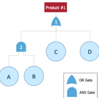
procured by the firm. As an example, let’s consider a product that a firm wishes to produce, Product
149
#1. Its bill of materials consists of three subassemblies supplied by four suppliers, A, B, C, and
150
D. The procurement for one of the subassemblies used in Product #1 will be divided between two
151
suppliers, A and B. If either Supplier A or Supplier B deliver their respective products on time the
152
supply chain is successful. Suppliers C and D are sole sources for the remaining two subassemblies.
153
In the construction of the fault tree, higher level events are associated with lower level and
154
parallel events through gates. OR-gates and AND-gates are two types of gates that are commonly
155
used in fault trees and are used to represent single/sole source situations and multiple sources of
156
supply respectively for the supply chain. Figure 1 illustrates the fault tree for Product #1’s supply
157
chain.
158
Figure 1: Supply chain represented as a fault tree.
159
The output of an OR-gate occurs if at least one of the input events occurs where the probability of
160
failure (unreliability) can be calculated as1−Q
j∈J(1−uj). AND-gates are used to model events that
161
must occur simultaneously in order for the output event to occur and correspond to a parallel system
162
where the unreliability is calculated as the product of independent event probabilities, Q
j∈Juj.
163
(Lindhe et al. , 2009)
Next, we consider the unreliability of the individual suppliers, uj, which is an estimate of the
165
probability that the supplier will not deliver their respective product or service on-time and j
166
is defined as the combination of the supplier and product/service that the particular supplier is
167
responsible for delivering. Throughout this paper, we have outlined cases where suppliers only
168
provide one product or service, which is reasonable given the case studies. However, the models
169
could easily accommodate suppliers that provide multiple products or services. In those cases, each
170
product or service would be represented by a different index j for the given supplier. Table 1
171
summarizes the unreliabilities forj = A, B, C, and D.
172
Table 1: Unreliabilities of suppliers. Supplier (j) Supplier unreliability(uj)
A 0.025
B 0.001
C 0.050
D 0.090
173
Within a fault tree, the combination of basic events that can cause the top event to occur is
174
called a cut set. Multiple cut sets may occur within any given fault tree. A minimal cut set is the
175
combination of basic events that result in the top event. In other words, minimal cut sets represent
176
all the shortest ways that the basic events can cause the top event. The set of minimal cut sets
177
can be obtained for any of the intermediate events (events common to the same gate) or overall for
178
the top event in the fault tree. As the number of events and complexity increases within the fault
179
tree, the use of algorithms becomes more important to efficiently identify the cut sets and minimal
180
cut sets in particular. Examples of such algorithms have been based on binary decision diagrams
181
and reliability block diagrams and include CARA, Shannon’s decomposition, and MOCUS among
182
others. (Veseleyet al. , 2002; Rosenberg, 1996)
183
Using Figure 1 as an example, the top-level event can be expressed as a Boolean function and
184
reduced to its primary input events by starting at the top of the fault tree and working downward.
185
The • indicates an AND gate,+ indicates an OR gate, andG designates the respective gate (G1,
186
G2).
Top-Level =G1 +G2
= (C+D) +G2
= (C+D) + (A•B)
In the above example, three cut sets result - A•B,C, and D. Because of the simplicity of the
188
example, each cut set is also a minimal cut set comprised of only basic events. Each of the minimal
189
cut sets define an event or series of events whose existence will initiate the top-level event in the
190
fault tree (Veseley et al. , 2002).
191
To calculate cut set unreliability, the unreliabilities of events within the same minimal cut sets
192
connected by AND gates are multiplied and those connected by OR gates are added. The result is
193
the unreliability of each cut set(Ui). By applying the rare event approximation(uj <0.1)(Veseley
194
et al. , 2002) and given that the top event unreliability is the union of the minimal cut sets, we
195
can sum the individual minimal cut set unreliabilities to obtain the unreliability of the top event in
196
the fault tree, UREA
S =
P
Ui; where US is the unreliability of the system being studied and REA
197
denotes that US was calculated using the rare event approximation. Since the probability of each
198
cut set (UA•B= 0.0000125,UC = 0.05, and UD = 0.090) is less than 0.1, the probability of having
199
two or more cut sets occur (e.g., C and D) is extremely small. Thus, according the rare event
200
approximation, we can calculate the union of the probabilities as the sum of the probabilities. In
201
the above example,UREA
S =UA•B+UC+UD ≈0.1400. Likewise, the reliability of the supply chain 202
for Product #1, RS, is equivalent to1− US and is≈0.8600.
203
In the second integer program, which is referred to later as the imperfect mitigation model, we
204
apply an alternative analysis procedure for fault trees based on the use of binary decision diagrams
205
that identifiesspecificsuppliers to mitigate. A binary decision diagram is constructed from the fault
206
tree of interest and is a directed acyclic graph in which all paths through the binary decision diagram
207
are in one direction and no loops can exist. The binary decision diagram consists of terminal and
208
non-terminal nodes connected by branches. Terminal nodes correspond to the final state of the
209
system (failure or success) and non-terminal nodes correspond to the basic events of the fault tree.
210
(Andrews & Rementy, 2005)
Several methods have been proposed to convert fault trees to binary decision diagrams. Within
212
this paper, we apply the component connection method (Andrews & Rementy, 2005). The process
213
consists of three primary steps: 1) ordering, 2) construction/connection, and 3) simplification. For
214
basic events that are connected through AND-gates, the corresponding nodes on the binary decision
215
diagram are connected to each other through the 1-branch of the node. Alternatively, for basic events
216
that are connected via OR-gates, the nodes that represent the basic events on the binary decision
217
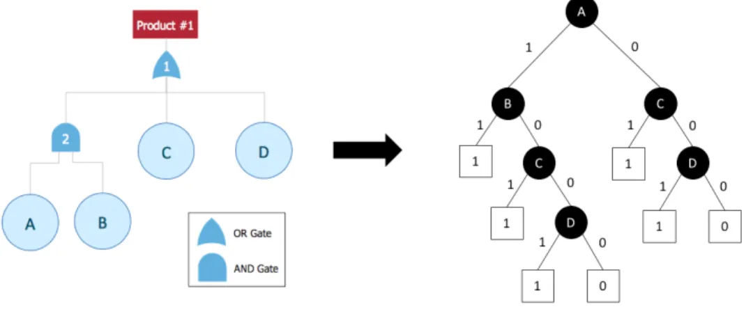
diagram are connected to each other on the 0-branch of the node. Figure 2 illustrates the conversion
218
of the fault tree that represents the supply chain of Product #1 (Figure 1) into a binary decision
219
diagram using the component connection method.
220
Figure 2: Example of converting a fault tree to a binary decision diagram.
The resulting binary decision diagram consists of nodes that represent basic events and have
221
associated probabilities of success (reliability) and probabilities of failure (unreliability) over a given
222
time period. Reliability paths are connected via 0-branches and unreliability paths are connected
223
via 1-branches. Paths that consist of the sequence of connections between basic events are cut sets
224
from the original fault tree and terminate at either a terminal 1 node or a terminal 0 node. Paths
225
that lead to a terminal 1 node specify the basic events (suppliers) for the top event in the fault
226
tree to occur. In the example presented above, A → B → C is one of the terminal 1 paths and
227
A → C → D is one of the terminal 0 paths. If redundancies within the binary decision diagram
228
have been removed, the basic events (suppliers) contained within a path terminating in a terminal 1
229
node lie along the fault tree’s minimal cut sets (Andrews & Dunnett, 2000). Conversely, the paths
230
that terminate in a terminal 0 node indicate top event nonoccurence.
We define Pj,`(j,ω) as the probability of supplier j in path ω being in state `. The supplier
232
is in state ` = 0 if the supplier is in a reliable state and in state ` = 1 if the supplier is in an
233
unreliable state. The index `(j, ω) represents the state of supplier j in path ω. Hereafter, the
234
notation Pj,`(j,ω) is simplified as Pj,ω since `(j, ω) is uniquely identified by j and ω. Let Ω be the
235
set of all terminal 1 node paths. Using the binary decision diagram approach, for a given terminal
236
1 path (ω) we can multiply the probabilities of all suppliers contained within that path (Jω) to
237
obtain the unreliability of that path. Subsequently we can take the summation across all terminal
238
1 paths to compute the top event (system) unreliability. For the example presented in Figure 2,
239
the resulting top event unreliability can be computed asP
ω∈Ω
Q
j∈Jω Pj,ω whereΩ ={1,2,3,4,5},
240
J1 ={A, B},J2 ={A, B, C},J3 ={A, B, C, D},J4={A, C},J5 ={A, C, D}, and the probability
241
of supplier j in path ω is a value that depends on one of two states, ` = {0,1}. The computed
242
unreliability using this method is ≈ 0.1355 or a reliability of ≈ 0.8645, which is slightly different
243
than the reliability computed above. The difference in the unreliability between these two methods
244
is a result of the first method employing the rare event approximation.
245
4
Problem Description and Model Formulations
246
4.1 Problem description
247
The problem that we consider in this research is relevant and practical. A supply chain manager
248
within the supply chain seeks to use resources as effectively as possible to mitigate risks with specific
249
suppliers. Supplier risk can be mitigated by performing various actions (e.g., additional oversight
250
is provided, the supplier is engaged in improvement activities, redundant suppliers are considered),
251
each of which reduce the probability that the supplier is late and each of which costs resources. The
252
manager seeks to minimize the unreliability (maximize the reliability) of the entire supply chain
253
under their responsibility while staying within a prescribed mitigation budget.
254
We approach the problem in two ways by formulating nonlinear integer programs that are
255
subsequently reformulated into linear integer programs with the aim of improving computational
256
efficiency. First, we develop aperfect mitigation model that aims at identifying areas of the supply
257
chain that are at-risk. The next model described, which we refer to as the imperfect mitigation
258
model, extends the perfect mitigation model by identifying specific mitigating actions to take on
specific suppliers to improve the overall reliability of the supply chain system.
260
4.2 Model Formulations
261
4.2.1 Perfect Mitigation Model
262
For the purposes of this paper, perfect mitigation occurs when an activity is taken that sets the
263
reliability of the cut set equal to 100%. In our formulation of the perfect mitigation model, we assume
264
that events (and subsequently minimal cut sets) are independent. This is a practical assumption
265
given that the factors that affect reliability within the supply chain studied have been shown not to
266
have a high degree of correlation (Sherwinet al. , 2016). By assuming mutually independent events,
267
we are able to apply Boolean algebraic operations and calculate the probability of occurrence that
268
at least one mode of failure (i.e., minimal cut set) within the fault tree will occur (Vesely, 2002). As
269
a result, the probability of failure of the top event of the fault tree can be stated as1−Q
i∈I(1−Ui)
270
where (1−Ui) is the probability that cut set i does not occur and I is the set of all minimal cut
271
sets.
272
The objective function (Eq. (1)) of a nonlinear integer program is formulated based on the above
273
assumption and using the binary decision variablexi; wherexi = 1if minimal cut setiis mitigated
274
and xi = 0 otherwise. Cut sets are linked to basic events (suppliers) via the model constraints
275
and specifically a second binary variable yj; where yj = 1 if supplier j is mitigated and yj = 0
276
otherwise. J is defined as the set of all basic events (suppliers). Ji represents the set of suppliers
277
that are members of cut set i. A budget value,b, is included in the formulation and represents the
278
mitigation budget of the firm and is compared to the cost, cj, of mitigating supplierj. The basis
279
for cj and its extension cjk are discussed in a later section. Given this notation, the objective for
280
minimizing the supply chain reliability can be represented as follows:
281
Minimize 1−Y
i∈I
(1−Ui)1−xi (1)
By converting the minimization to a maximization and taking the logarithm of the objective
282
function, the perfect mitigation model is reformulated as follows:
Maximize X i∈I log(1−Ui)(1−xi) (2) s.t. xi ≤ X j∈Ji yj ∀i∈I, (3) X j∈J cjyj ≤b (4) xi ∈ {0,1} ∀i∈I (5) yj ∈ {0,1} ∀j∈Ji (6)
Subsequently, the resulting supply chain reliability is computed by applying the exponential
284
function to Objective Function (2):
285 exp " Maximize X i∈I log(1−Ui)(1−xi) # (7)
Constraint (3) enforces that a minimal cut set can only be mitigated if at least one of its suppliers
286
is mitigated and Constraint (4) enforces the budget for supplier mitigation. As mentioned above,
287
this model assumes that if a supplier is mitigated then it is 100% reliable, an impractical assumption
288
in many cases. In even the best circumstances, it is rare that a supplier will become perfectly reliable
289
after completing mitigation actions. As a result, the perfect mitigation model computes a best-case
290
bound and can serve as a means for practitioners to identify the areas or groups of suppliers of
291
highest risk within the supply chain system.
292
4.2.2 Imperfect Mitigation Model
293
Whereas the perfect mitigation model describes perfect supplier intervention, we now introduce an
294
imperfect mitigation model that selects individual suppliers to mitigate. In this example, supplier
295
intervention reduces, but does not eliminate, the chance of supplier unreliability. Examples of such
296
intervention activities that we will explore include taking action to improve the existing supplier’s
297
reliability, replacing the supplier with an improved supplier, providing additional oversight to assist
298
the supplier, or taking no mitigation action at all. All of the supplier-specific activities described
are intended to have a favorable impact on the overall reliability of the supply chain system and
300
represent actual activities that are applied in industry settings.
301
For the imperfect mitigation model we convert the fault tree that represents the supply chain
302
system into a binary decision diagram. This approach leverages the computational advantages of
303
the binary decision diagram structure as well as more effectively models the problem such that
304
individual suppliers can be identified as targets for risk mitigation activities.
305
The imperfect mitigation model is developed similarly to the perfect mitigation model, but is
306
based on the binary decision diagram that has been converted from the fault tree that represents the
307
supply chain structure being analyzed. The objective function is formulated as part of a nonlinear
308
integer program and seeks to minimize the overall unreliability of the supply chain system. We
309
introduce an indexkto represent the mitigation activity performed on a supplier. More specifically,
310
Pj,ω,k is the probability that supplierjalong pathωdoes not deliver on-time if mitigation activityk
311
was performed on supplierj. A binary decision variableyjk is introduced and represents whether or
312
not supplierjis mitigated using actionk. The selection of mitigation activitykreduces unreliability,
313
but does not necessarily reduce the unreliability to 0%. Subsequently, taking the summation across
314
all terminal 1 paths(ω∈Ω)within the binary decision diagram results in the top event unreliability,
315
or system unreliability. Thus, the model is as follows.
316 Minimize X ω∈Ω Y j∈Jω Y k∈K Pyj,ω,kjk (8) s.t. X j∈J X k∈K cjkyjk ≤b (9) X k∈K yjk = 1 ∀j∈J (10) yjk ∈ {0,1} ∀j∈J;k∈K (11)
The objective function (8) represents the summation of the product of the unreliabilities of the
317
path sets within the binary decision diagram. Constraint (9) is a budgetary constraint (b) and
318
second constraint (10) assures that, if selected, a supplier (j) is only subject to one mitigation
319
activity(k).
320
In the imperfect mitigation model formulation, we extend the cost function values (cjk) used
in Constraint (9) specific to the mitigation activity chosen. By taking this approach, we are able
322
to choose the optimal mitigation activities to take with individual suppliers that minimizes the
323
unreliability of the supply chain system being studied within the budgetary constraints set by the
324
firm.
325
Next, we present a linearized reformulation of the imperfect mitigation model that exactly
326
resolves the nonlinear terms at the expense of adding variables. Specifically, we introduce variables
327
wω
rk, which we will refer to as the partial probability associated with each path ω,r holds an index
328
for therth supplier on the path, andkis the mitigation activity applied to therth supplier. These
329
variables represent the quantity, Pj(1,ω),`(1,ω),k(1,ω)Pj(2,ω),`(2,ω),k(2,ω)...Pj(r,ω),`(r,ω),k(r,ω), which is the
330
probability that the firstrsuppliers within pathωrealize the respective fail/no-fail state (`) assigned
331
to them within the path given thatk(r, ω)is the mitigation level forrthsupplierjin pathω. Given
332
that |Jω| is the index of the last supplier in path ω, w|ωJω|,k holds the product of all of the facility
333
probabilities, which is equal to the probability of pathω. As a result, we can reformulate our model
334 as follows. 335 Minimize X ω∈Ω X k∈K wω|Jω|,k (12) s.t. wω1k=Pj(1,ω),`(1,ω),k(1,ω)yj(1,ω),k ∀k∈K; ω∈Ω; `∈ {0,1} (13) X k∈K wrω−1,k= X k∈K 1 Pj(r,ω),`(r,ω),k(r,ω) wωrk ∀ω∈Ω; ∀j ∈J; r= 2, ...,|Jω|; `∈ {0,(14)1} 0≤wωrk≤yj(r,ω),k ∀j∈J; k∈K; r ∈R; ω∈Ω (15) X j∈J X k∈K cjkyjk ≤b (16) X k∈K yjk = 1 ∀j∈J (17) yjk ∈ {0,1} ∀j∈J; k∈K (18)
The objective function (12) is the summation of the probabilities of all scenarios that result in a
336
failure, which is equivalent to the supply chain reliability. Constraints (13) are “probability chain”
337
constraints that compute the realization probability of the first supplier (r= 1) in each path given
338
the value of the mitigation decision variable,yj(1,ω),k . In these constraints variablewω1kcorresponds
339
to the first facility in path ω (note that this facility is in state `(r, ω) in path ω). The variable
wω1k equals the probability that this first facility is in state`(r, ω) when mitigation k is applied to
341
this facility (i.e., Pj(1,ω),`(1,ω),k(1,ω)) if yj(1,ω),k = 1 and zero otherwise. For each path, the second
342
constraint (14), also forming a probability chain, computes the (r−1)th partial probability (wrω−1,k
343
for some value ofk) by taking the product ofrth partial probability (wωrk for some value ofk) and
344
the inverse of the probability that the rth supplier is in state ` on the path (Pj(r,ω),`(r,ω),k(r,ω) for
345
some value of k); this “chain” starts with the second supplier in the path and continues to the last
346
supplier. In this way, the partial probability of the last supplier in a pathω (wω
|Jω|,k) is the product
347
of the state probabilities of all of the suppliers in the path. The third constraints (15) assure that
348
the partial probability variableswrkω are non-negative, but yet positive only if mitigationkis applied
349
to therth supplier in pathω (i.e.,yj(r,ω),k= 1). The fourth constraint (16) serves as the budgetary
350
constraint, and the fifth constraint (17) assures that only one mitigation activity (k) is selected for
351
each supplier (j).
352
The rationale for this linearized model is as follows. Let k∗(j) be the mitigation level selected
353
for supplier j in the optimal solution (i.e., the value of k for which yjk = 1). Then the recursive
354
Equations (19) (which correspond to (14) above) represent the partial probabilities of each path (ω)
355
for r= 2, . . . ,|Jω|.
356
Pj(r,ω),`(r,ω),k∗(r,ω)wr−1,k∗(r−1)=wω
rk∗(r) r = 2, ...,|Jω|; ω∈Ω (19)
To show that Equation (14) results in Equation (19), consider the following example. Suppose
357
that supplier r−1 is mitigated by choosing k= 2 and supplier r by choosing mitigation activity
358 k= 1. Expanding (14) we obtain: 359 wrω−1,1+wωr−1,2= 1 Pj(r,ω),`(r,ω),1 wrω1+ 1 Pj(r,ω),`(r,ω),2 wrω2 r= 2, ...,|Jω|; ω∈Ω (20) Because wrω−1,1 = 0 andwrω2 = 0, 360
wωr−1,2 =
1
Pj(r,ω),`(r,ω),1
wωr1 r= 2, ...,|Jω|; ω∈Ω (21)
Rearranging Equation (21) yields the recursive equation in the format shown in Equation (19):
361
Pj(r,ω),`(r,ω),1wr−1,2=wrω1 r= 2, ...,|Jω|; ω∈Ω (22)
5
Motivating Example: Nuclear Power Plant Supply Chain
362
Firms, like those in the nuclear power industry, that produce a low volume of high value (LVHV)
363
goods with long lead times are sensitive to supply chain disruptions since they do not have the luxury
364
of inventory buffers to mitigate late deliveries due to higher cost items, lower production quantities,
365
and less frequent deliveries. LVHV industries are studied less in supply chain risk management
366
literature, but represent important industries in the U.S. economy, defense industry, and global
367
economy overall. Examples of LVHV industries include aircraft, shipbuilding, and power plant
368
construction, which are reported to have global market sizes of $1.96 trillion, $258 billion, and $4.78
369
trillion respectively (Aboulafia, 2017; Geaney et al. , 2015; Dyble, 2018).
370
Nuclear power plant construction supply chains are a good example of an LVHV industry, which
371
are characterized by long lead times, demand for increasingly scarce capabilities, and fewer and
372
fewer suppliers that are qualified to meet the stringent requirements. These characteristics create
373
significant risk for firms within the nuclear power plant construction supply chain. The risks are
374
confounded due to the low volume, costly barriers to entry, and relatively infrequent demand, which
375
disincentivizes new firms from participating in the supply chain. Thus, LVHV firms like those in
376
the nuclear industry are especially vulnerable to supply chain risks. These challenges that nuclear
377
power plant construction supply chains face appear frequently in other LVHV supply chains such
378
as the defense industrial base and aerospace.
379
Although the models developed in this paper could apply to other supply chains, they are
380
quite appropriate for LVHV supply chains primarily due to the aforementioned factors and the
381
long lead times that these industries experience. The long lead times are a consequence of the
complexity and time that the projects take to design and manufacture. As a result, both suppliers
383
and customers make long term commitments to one another and within their respective businesses
384
to ensure they are qualified and capable to make such products. These characteristics, combined
385
with the fact that these supply chains are comprised of several tiers, requires a significant level
386
of coordination within the supply chain system to assure products are delivered on-time and with
387
the requisite quality. For example, a British nuclear submarine can take 14 years to design and
388
build at a cost of $1.6 billion (BBC, 2014). When suppliers fail to deliver equipment on-time,
389
the completion of the end product can be significantly late and result in liquidated damages. In
390
high volume supply chains, suppliers make deliveries more frequently, the deliveries are in higher
391
quantities, buffer inventory levels are maintained, and the supply chain is typically comprised of a
392
distributed network of suppliers. The typical risk management solutions for higher volume supply
393
chains (inventory buffers, transportation networks, site selection, and constructing optimal response
394
plans) may not be applicable to LVHV supply chains because of the unique risk exposure that results
395
from a scarce supply of capable providers, low quantities of demand, significant capital investment,
396
and long lead times to manufacture such goods. Therefore, LVHV supply chains require models
397
that proactively identify and mitigate risks in order to improve reliability.
398
In the sections that follow, the models presented above are applied at two levels within the
399
same supply chain. The first level analyzes the basic supply chain used in nuclear power plant
400
construction. The second level supply chain is based on the perspective of a supplier to the firm
401
constructing the nuclear power plant and consists of a turbine, which is a key component used
402
within the nuclear power plant. These examples demonstrate the flexibility of the approach in that
403
it enables the decision maker to either take a broader system view of the supply chain or a modular
404
view and include or exclude portions of the supply chain during their analysis.
405
5.1 Supply chain definition
406
We have chosen a pressurized water reactor as the basis for the bill of materials of the nuclear power
407
plant because several nuclear power plants based on the pressurized water reactor design are being
408
constructed worldwide (WNA, 2018). Further, our focus is on the primary items sourced for the
409
plant. We exclude building materials and other items in order to simplify the application. The
410
following items are included in the pressurized water reactor bill of materials used in our analysis
in the pages that follow: containment structure, pressurizer, steam generator, control rods, reactor
412
vessel, steam turbine, generator, and condenser.
413
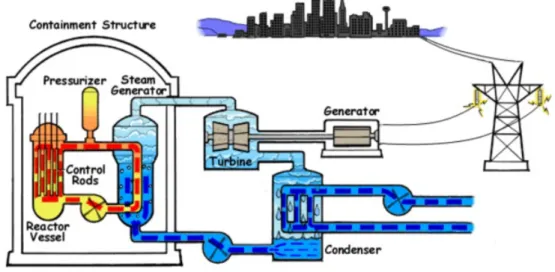
One of the primary items in the pressurized water reactor is the steam turbine. Within the
414
reactor vessel, the core creates heat. The heat is then transferred via the primary coolant loop to
415
the steam generator where water is vaporized and produces steam. The steam is directed to the
416
main turbine, causing it to turn the turbine generator, which results in electrical power production.
417
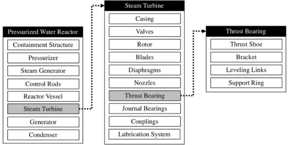
(USNRC, 2015) Steam turbine designs vary. However, the primary components of a steam turbine
418
include the casing, valves, a rotor containing blades, diaphragms, nozzles, and a host of other
419
auxiliary equipment that comprise the turbine system. Examples of auxiliary equipment include
420
thrust bearings, journal bearings, couplings, and lubricating systems. For the purposes of this study,
421
we will examine a steam turbine thrust bearing. Figure 3 shows a schematic of a pressurized water
422
reactor and its primary items. Figure 4 outlines the flow of the bills of material for the pressurized
423
water reactor, steam turbine, and thrust bearing that will be used in the computational studies that
424
follow.
425
Figure 4: Bills of material.
5.2 Fault tree and binary decision diagram formulation
426
5.2.1 Pressurized water reactor
427
For the pressurized water reactor supply chain, we take the perspective of the construction firm
428
responsible for sourcing the primary goods and services for the pressurized water reactor. In the
429
examples presented, we assume that multiple pressurized water reactors are being built
simultane-430
ously. As a result, dual-sourcing positions across the multiple pressurized water reactor construction
431
sites exist for some, but not all of the goods and services being procured by the construction firm.
432
The pressurized water reactor supply chain consists of the eight primary goods and services provided
433
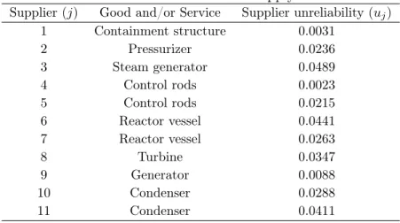
by eleven suppliers. Table 2 outlines the suppliers(j), their respective goods and services, and the
434
supplier’s unreliability (uj). The unreliability numbers, which are equivalent to the late delivery
435
percentage, presented here are synthetic, but are reflective of unreliabilities experienced within the
436
nuclear industry.
Table 2: Pressurized water reactor supply chain data.
Supplier(j) Good and/or Service Supplier unreliability(uj) 1 Containment structure 0.0031 2 Pressurizer 0.0236 3 Steam generator 0.0489 4 Control rods 0.0023 5 Control rods 0.0215 6 Reactor vessel 0.0441 7 Reactor vessel 0.0263 8 Turbine 0.0347 9 Generator 0.0088 10 Condenser 0.0288 11 Condenser 0.0411
The resulting fault tree for the pressurized water reactor can be found in Figure 5. Each of
438
the goods and services provided are represented by basic events and the respective suppliers that
439
provided them. Basic events that are inputs to the three AND gates in the fault tree include
440
control rods, the reactor vessel, and the condenser. AND gates represent situations where the
441
firm constructing the pressurized water reactor has chosen dual source options. The containment
442
structure, pressurizer, steam generator, turbine, and generator are being provided by single sources
443
of supply in this example and the basic events that represent them are connected via OR gates in
444
the fault tree.
Figure 5: Pressurized water reactor fault tree.
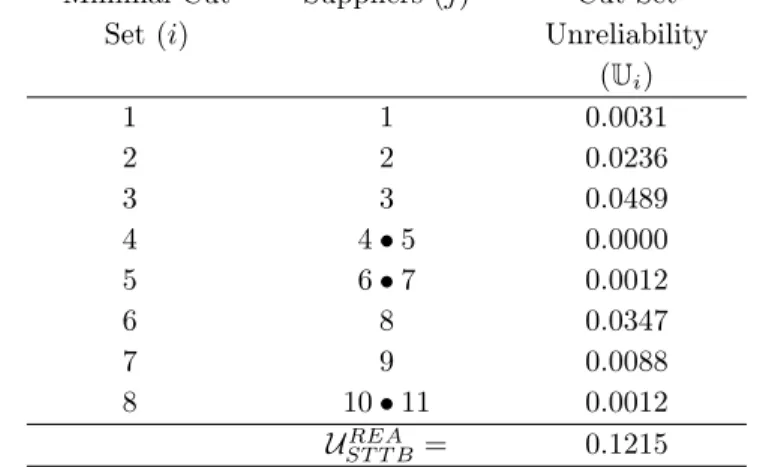
A total of eight cut sets (i= 1, ...,8)result from the pressurized water reactor fault tree. Each
446
cut set is a minimal cut set, which represents an event or series of events whose occurrence will result
447
in the realization of the top event of the fault tree (Veseleyet al., 2002). Using the data presented
448
in Table 2 and the rare event approximation, the pressurized water reactor supply chain system
449
unreliability is UREA
P W R = 0.1215. Table 3 includes the minimal cut sets and associated minimal cut
450
set unreliabilities for the pressurized water reactor fault tree.
451
Table 3: Pressurized water reactor fault tree minimal cut set data.
Minimal Cut Set(i)
Suppliers(j) Cut Set Unreliability (Ui) 1 1 0.0031 2 2 0.0236 3 3 0.0489 4 4•5 0.0000 5 6•7 0.0012 6 8 0.0347 7 9 0.0088 8 10•11 0.0012 UREA ST T B = 0.1215
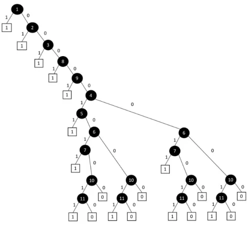
Next, we construct a binary decision diagram using the component connection method. The
452
binary decision diagram structure is used as input to the imperfect mitigation models as described
453
above. Figure 6 is a graphical representation of the binary decision diagram based on the fault tree
454
shown in Figure 5 where nodes represent suppliers.
455
Figure 6: Binary decision diagram for pressurized water reactor fault tree.
5.2.2 Steam turbine thrust bearings
456
Steam turbine thrust bearings are used as a primary component in the steam turbine (j= 8 in the
457
pressurized water reactor fault tree). In constructing the fault tree for the thrust bearing, we take
458
the perspective of the firm who is the supplier to the steam turbine manufacturer. In our example,
459
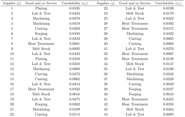
the thrust bearing manufacturer’s supply chain consists of 44 suppliers (see Table 4 for individual
460
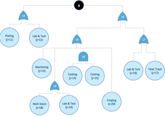
supplier unreliabilities) and the resulting fault tree consists of 31 gates, which is shown in Figure 7.
Table 4: Steam turbine thrust bearing supply chain data.
Supplier(j) Good and/or Service Unreliability(uj) Supplier(j) Good and/or Service Unreliability(uj)
1 Plating 0.0195 23 Lab & Test 0.0199
2 Lab & Test 0.0424 24 Melt Stock 0.0178 3 Machining 0.0379 25 Lab & Test 0.0322 4 Machining 0.0419 26 Heat Treatment 0.0492
5 Casting 0.0203 27 Heat Treatment 0.0157
6 Forging 0.0450 28 Machining 0.0422
7 Lab & Test 0.0323 29 Casting 0.0065
8 Heat Treatment 0.0081 30 Casting 0.0062
9 Melt Stock 0.0092 31 Lab & Test 0.0276 10 Lab & Test 0.0433 32 Heat Treatment 0.0097
11 Plating 0.0459 33 Heat Treatment 0.0129
12 Lab & Test 0.0316 34 Melt Stock 0.0147 13 Machining 0.0009 35 Lab & Test 0.0190
14 Casting 0.0472 36 Machining 0.0343
15 Casting 0.0062 37 Machining 0.0328
16 Lab & Test 0.0454 38 Casting 0.0049
17 Heat Treatment 0.0332 39 Forging 0.0107
18 Melt Stock 0.0016 40 Forging 0.0010
19 Lab & Test 0.0475 41 Heat Treatment 0.0425
20 Forging 0.0362 42 Heat Treatment 0.0358
21 Machining 0.0189 43 Melt Stock 0.0484
22 Casting 0.0114 44 Lab & Test 0.0095
Figures 7 through 12 illustrate the supply chains as fault trees for the items used in the
manufac-462
ture of the thrust bearing. These items include the thrust shoe, bracket, leveling links, and support
463
ring. Thrust shoes are sourced from two separate suppliers. All other top-level items (bracket,
464
leveling links, support ring) are procured from single or sole sources.
Figure 7: Steam turbine thrust bearing manufacturer top-level fault tree.
466
467
Figure 9: Thrust shoe supply chain (Source B).
468
Figure 10: Bracket supply chain (Source C).
Figure 11: Leveling link supply chain (Source D).
470
Figure 12: Support ring supply chain (Source E).
471
A total of 99 minimal cut sets are contained within the thrust bearing fault tree. We again
472
apply the rules of Boolean algebra and the rare event approximation. The resulting steam turbine
thrust bearing supply chain system unreliability is UREA
ST T B = 0.3128. This translates to a 31.28%
474
probability of not being completed on-time as the result of delivery failures within the supply chain.
475
Table 5 summarizes the unreliability data of the steam turbine thrust bearing supply chain fault
476
tree minimal cut sets.
477
Figure 13 shows a portion of the overall binary decision diagram developed from the steam
478
turbine thrust bearing fault tree and specifically the suppliers that comprise the thrust shoe supply
479
chain (see Figure 8). After applying simplification rules (Andrews & Rementy, 2005), the steam
480
turbine thrust bearing binary decision diagram consists of a total of 99 paths.
Table 5: Steam turbine thrust bearing fault tree minimal cut set data. Minimal Cut Set (i) Suppliers (j) Cut Set Unreliability (Ui) Minimal Cut Set (i) Suppliers (j) Cut Set Unreliability (Ui) Minimal Cut Set (i) Suppliers (j) Cut Set Unreliability (Ui) 1 1•11 0.00089505 34 9•20 0.00033304 67 7•18 0.00005168 2 1•12 0.00061620 35 9•16 0.00041768 68 7•19 0.00153425 3 1•13 0.00001755 36 9•17 0.00030544 69 7•14•15 0.00000945 4 1•18 0.00003120 37 10•11 0.00198747 70 7•20 0.00116926 5 1•19 0.00092625 38 10•12 0.00136828 71 7•16 0.00146642 6 1•14•15 0.00000571 39 10•13 0.00003897 72 7•17 0.00107236 7 1•20 0.00070590 40 10•18 0.00006928 73 8•11 0.00037179 8 1•16 0.00088530 41 10•19 0.00205675 74 8•12 0.00025596 9 1•17 0.00064740 42 10•14•15 0.00001267 75 8•13 0.00000729 10 2•11 0.00194616 43 10•20 0.00156746 76 8•18 0.00001296 11 2•12 0.00133984 44 10•16 0.00196582 77 8•19 0.00038475 12 2•13 0.00003816 45 10•17 0.00143756 78 8•14•15 0.00000237 13 2•18 0.00006784 46 5•11 0.00093177 79 8•20 0.00029322 14 2•19 0.00201400 47 5•12 0.00064148 80 8•16 0.00036774 15 2•14•15 0.00001241 48 5•13 0.00001827 81 8•17 0.00026892 16 2•20 0.00153488 49 5•18 0.00003248 82 21 0.01890000 17 2•16 0.00192496 50 5•19 0.00096425 83 24 0.01780000 18 2•17 0.00140768 51 5•14•15 0.00000594 84 25 0.03220000 19 3•4•11 0.00007289 52 5•20 0.00073486 85 22 0.01140000 20 3•4•12 0.00005018 53 5•16 0.00092162 86 23 0.01990000 21 3•4•13 0.00000143 54 5•17 0.00067396 87 26 • 27 0.00077244 22 3•4•18 0.00000254 55 6•11 0.00206550 88 28 0.04220000 23 3•4•19 0.00007543 56 6•12 0.00142200 89 31 0.02760000 24 3•4•14•15 0.00000046 57 6•13 0.00004050 90 32 0.00970000 25 3•4•20 0.00005749 58 6•18 0.00007200 91 29 • 30 0.00004030 26 3•4•16 0.00007210 59 6•19 0.00213750 92 33 0.01290000 27 3•4•17 0.00005272 60 6•14•15 0.00001317 93 34 • 35 0.00027930 28 9•11 0.00042228 61 6•20 0.00162900 94 36 • 37 0.00112504 29 9•12 0.00029072 62 6•16 0.00204300 95 43 0.04840000 30 9•13 0.00000828 63 6•17 0.00149400 96 44 0.00950000 31 9•18 0.00001472 64 7•11 0.00148257 97 38 0.00490000 32 9•19 0.00043700 65 7•12 0.00102068 98 39 • 40 0.00001070 33 9•14•15 0.00000269 66 7•13 0.00002907 99 41 • 42 0.00152150 UREA ST T B = 0.31292916 482
Figure 13: Binary decision diagram for steam turbine thrust bearing thrust shoe (see Figure 8).
483
5.3 Mitigation Cost
484
The cost of mitigating the risks of supplier j is a function of the time estimated for the mitigation
485
activity (k) and the hourly rate of personnel to complete the activity (h= $104 per hour (USBLS,
486
2015)). The respective costs used for the four mitigation activities available are described in Table
487
6 and were estimated empirically based on industry knowledge.
488
Table 6: Cost function values.
Mitigation Activity k Reliability
Improve-ment
cjk
Improve the existing supplier 1 15% $12,209
Replace supplier with an improved supplier 2 25% $27,737 Increase oversight at existing supplier 3 5% $10,816
In order to maintain consistency between the perfect mitigation model and the imperfect
miti-489
gation model for comparison purposes, we have set the mitigation cost (cj) in the perfect mitigation
490
model to $12,209, which is equivalent to cj1 in the imperfect mitigation model even though the
491
functions described in Table 6 do not apply to the perfect mitigation model.
492
6
Computational Results
493
For the supply chains described above, we run the models outlined using data representative of the
494
nuclear industry. Although the perfect mitigation model provides less information to the
practi-495
tioner than the imperfect mitigation model, it can be notionally useful to identify areas of concern
496
(suppliers to focus on when planning mitigation efforts) within the supply chain. Once those areas
497
of concern are identified, the practitioner may choose the specific mitigation activities to perform
498
for each individual supplier.
499
The computational results are presented in a fashion relevant to the supply chain professional
500
who, with a limited budget, will be challenged with minimizing risk across the supply chain system
501
that he/she is managing. As a result, each model is run at $10,000 budgetary increments up to a
502
maximum budget of $300,000 or an overall system reliability of 100% (0% unreliability), whichever
503
comes first. Results are presented as a Pareto frontier and demonstrate the optimal tradeoff between
504
the budget allocation and resulting reliability of the supply chain system being analyzed.
505
Both the pressurized water reactor and steam turbine thrust bearing supply chains are analyzed
506
in the pages that follow utilizing each of the modeling approaches outlined throughout this paper.
507
6.1 Perfect Mitigation
508
Here, we analyze the supply chains using the perfect mitigation model described in Objective
Func-509
tion (2) and Constraints (4)-(6). Figure 14 demonstrates the tradeoff between the system
relia-510
bility and mitigation cost for both the pressurized water reactor and steam turbine thrust bearing
511
supply chains independently. Prior to investing in mitigation activities, the reliability of the
pres-512
surized water reactor and steam turbine thrust bearing supply chains were RP M M
P W R = 0.8837 and
513
RP M M
ST T B = 0.7285respectively. At successive levels of investment, the reliability of each supply chain
514
system increases as expected. The pressurized water reactor supply chain achieves 100% reliability
at a cost of $109,881. The steam turbine thrust bearing does not achieve 100% reliability prior to
516
exhausting the $300,000 maximum budget. Instead, the thrust bearing supply chain sees a
max-517
imum reliability of 99.98% at a total cost of $293,016. In both cases, the marginal improvement
518
in system reliability decreases with increasing investment in mitigation activity. This information
519
could prove quite important to a practitioner responsible for allocating resources to minimizing
520
risk within a supply chain. For example, a supply chain manager might determine that budgeting
521
$150,000 to increase the reliability of the thrust bearing supply chain is satisfactory given that the
522
resulting improvement in reliability (to 95.12%) is sufficient.
523
Figure 14: System reliability improvement as a function of mitigation budget (perfect mitigation model).
Table 7 includes the minimal cut sets whose probabilities have been nullified and contain the
524
suppliers selected to mitigate for each formulation and within the pressurized water reactor supply
525
chain. Across all budgetary levels minimal cut set 4 was not chosen. This is reasonable given the
526
fact that the cut set is already 100% reliable without any mitigation. Table 8 includes the same
527
information in a summarized format for the steam turbine thrust bearing supply chain. Minimal cut
528
sets 6, 24, 33, 51, 78, 91, and 98 were not chosen by the model in the thrust bearing supply chain
529
system. These cut sets have relatively lower reliability values and at the same time are located
530
within regions of the fault tree/supply chain that have minimal impact on reducing the overall
system unreliability.
532
Table 7: Minimal cut sets selected in pressurized water reactor supply chain.
Budget Minimal Cut Set(s)
$10,000 – $20,000 3 $30,000 3, 6 $40,000 2, 3, 6 $50,000 1, 2, 3, 6 $60,000 1, 2, 3, 6 $70,000 2, 3, 6, 7 $80,000 1, 2, 3, 6, 7 $90,000 1, 2, 3, 6, 7, 8 $100,000 1, 2, 3, 5, 6, 7 $110,000 1, 2, 3, 5, 6, 7, 8
Table 8: Minimal cut sets selected in steam turbine thrust bearing supply chain.
Budget Minimal Cut Set(s)
$100,000 82, 83, 84, 86, 88, 89, 92, 95 $200,000 1, 5, 7-10, 14, 16-19, 23, 25-28, 32, 34-37, 41, 43-46, 50, 52-55, 59, 61-64, 68, 70-73, 77, 79-86, 88, 89, 90, 92, 95, 96 $300,000 1-5, 7-14, 16-23, 25-32, 34-41, 43-50, 52-59, 61-68, 70-77, 79-90, 92-97, 99 6.2 Imperfect Mitigation 533
Objective Function (12) and Constraints (13)-(17) constitute the formulation of the linearized
im-534
perfect mitigation model used to analyze the pressurized water reactor and steam turbine thrust
535
bearing supply chains. Prior to investment or taking any mitigating actions, the system
reli-536
abilities of the pressurized water reactor and steam turbine thrust bearing supply chains were
537
RIM M
P W R = 0.8836 and RIM MST T B = 0.7982 respectively. Figure 15 illustrates the tradeoff between
in-538
creasing investments in mitigating activities and the improvement in supply chain reliability. At a
539
total mitigation budget of $300,000 neither of the supply chains had achieved 100% system reliability
540
(RIM M
P W R = 0.9122, RIM MST T B = 0.8354).
Figure 15: System reliability improvement as a function of mitigation cost (imperfect mitigation model).
Table 9 illustrates the suppliers and mitigation activities selected at three budgetary levels for
542
the pressurized water reactor supply chain. Optimal mitigation activities at select budgetary levels
543
for the steam turbine thrust bearing supply chain are shown in Table 10. For both supply chains,
544
the mitigation action increase oversight at existing supplier (k = 3) was only chosen twice, at
545
b = $150,000 and b = $230,000, which was the least frequent of all mitigation options. Next to
546
selectingno mitigation activity (k= 4), increasing oversight at the existing supplier projected the
547
least impact on improving reliability (5%) at a relatively similar cost ($10,816) to improving the
548
existing supplier (k= 1), which cost $12,209and resulted in a reliability improvement of 15%.
549
Table 9: Suppliers selected in the pressurized water reactor supply chain.
Budget Supplier(s) k=1 k=2 k=3 k=4 $100,000 9 2, 3, 8 – 1, 4, 5, 6, 7, 10, 11 $200,000 5, 6, 7, 10, 11 1, 2, 3, 8, 9 – 4 $300,000 4 1, 2, 3, 5, 6, 7, 8, 9, 10, 11 – –
Table 10: Suppliers selected in the steam turbine thrust bearing supply chain. Budget Supplier(s) k=1 k=2 k=3 k=4 $100,000 31 25, 28, 43 – 1-24, 26, 27, 29, 30, 32-42, 44 $200,000 11, 16, 19, 21, 24 23, 25, 28, 31, 43 – 1-10, 12-15, 17, 18, 20, 22, 26, 27, 29, 30, 32-42, 44 $300,000 11, 16, 17, 19, 20, 22, 32, 33 21, 23, 24, 25, 28, 31, 43 – 1-10, 12-15, 18, 26, 27, 29, 30, 34-42, 44
Similar to the perfect mitigation model, the tradeoff between mitigation investment and
improve-550
ment in overall supply chain system reliability is useful to a practitioner. Compared to the perfect
551
mitigation model, the imperfect mitigation model provides additional flexibility since mitigation
552
activities for individual suppliers are chosen by the model. As a result, improvements in system
re-553
liability based on specific actions are observed up to the maximum budget allocated ($300,000) and
554
the practitioner is left to decide if the incremental investment is worth the additional improvement.
555
The additional flexibility that the imperfect mitigation model provides a supply chain
practi-556
tioner is evident in the activities chosen by the model. Generally, if mitigation funds are available,
557
the model seeks to maximize the use of those funds for a corresponding maximum benefit in system
558
reliability. As a result, the mitigation activities chosen and the suppliers chosen to mitigate change
559
at increasing budgetary levels depending on the cost-reliability tradeoff; a pattern that is observed
560
in both the pressurized water reactor and steam turbine generator supply chains.
561
6.3 Comparison of Mitigation Models and Formulations
562
Next, we compare the two mitigation models by analyzing the solution sets at the same budgetary
563
levels and the system reliabilities at the same budgetary levels for each of the supply chain systems
564
studied. The perfect mitigation model contains two decision variables,xiandyj, which represent the
565
cut sets containing suppliers and the suppliers chosen at each mitigation budget level respectively.
566
As a result, we are able to compare the solution sets of suppliers selected for the perfect and imperfect
567
mitigation models for each budgetary level. Tables 11 and 12 include a summary of the results of
568
the solution sets for both supply chains studied at select budgetary levels. Overall, the models