Open Works
Senior Independent Study Theses
2014
The Analytic Hierarchy Process: A Mathematical
Model for Decision Making Problems
Giang Huong Nguyen
The College of Wooster, [email protected]
Follow this and additional works at:https://openworks.wooster.edu/independentstudy Part of theMathematics Commons
This Senior Independent Study Thesis Exemplar is brought to you by Open Works, a service of The College of Wooster Libraries. It has been accepted for inclusion in Senior Independent Study Theses by an authorized administrator of Open Works. For more information, please contact
© Copyright 2014 Giang Huong Nguyen Recommended Citation
Nguyen, Giang Huong, "The Analytic Hierarchy Process: A Mathematical Model for Decision Making Problems" (2014).Senior Independent Study Theses.Paper 6054.
model for decision making
problems
IndependentStudyThesis
Presented in Partial Fulfillment of the Requirements for the Degree Bachelor of Arts in
the Department of Mathematics and Computer Science at The College of Wooster
by
Giang Huong Nguyen The College of Wooster
2014
Advised by: Dr. John Ramsay
The ability to make the right decision is an asset in many areas and lines of profession including social work, business, national economics, and
international security. However, decision makers often have difficulty choosing the best option since they might not have a full understanding of their preferences, or lack a systematic approach to solve the decision making problems at hand. The Analytic Hierarchy Process (AHP) provides a
mathematical model that helps the decision makers arrive at the most logical choice, based on their preferences. We investigate the theory of positive, reciprocal matrices, which provides the theoretical justification of the method of the AHP. At its heart, the AHP relies on three principles: Decomposition, Measurement of preferences, and Synthesis. Throughout the first five chapters of this thesis, we use a simple example to illustrate these principles. The last chapter presents a more sophisticated application of the AHP, which in turn illustrates the Analytic Network Process, a generalization of the AHP to systems with dependence and feedback.
I would like to thank Professor John Ramsay, my advisor, for his tremendous support with this thesis. His knowledge of the subject, passion for
mathematics, and relentless encouragement were the main source of motivation that got me through a research project that at times seemed impossible. Being his student has been the most extraordinary experience in my sixteen years of schooling. I am most grateful to complete an Independent Study project under his guidance.
My sincere thanks goes to all of the professors in the Department of Mathematics and Computer Science. Each of them has offered advice that helped shape the outcome of this thesis.
I would also like to thank my friends, Dung Nguyen’14 and Chris and Christy Ranney, for their support. Without them, this thesis would not have been possible.
Last but not least, thank you, Mom and Dad, for having faith in my abilities and judgment.
Abstract iii
Acknowledgements v
1 Introduction 1
1.1 Motivation . . . 1 1.2 The Initial Problem . . . 2 1.3 Research Outline . . . 6
2 The Consistent Decision Maker 9
2.1 The Eigenvalue Problem . . . 9 2.2 Finding the Weight Vector for the Alice Example . . . 16
3 The Inconsistent Decision Maker 19
3.1 From Consistent to Inconsistent . . . 19 3.2 Positive Matrices and Their Eigenvalues . . . 22 3.3 Finding the Weight Vector for the Inconsistent Alice Example . . 41
4.1 Finding the Score of Each Alternative in the Alice Example . . . . 46 4.2 The Hierarchy . . . 51 4.3 Extension of the Hierarchy in the Alice Example . . . 53
5 Metrics 59
5.1 Measure of Consistency . . . 60 5.1.1 Consistency of a Pairwise Reciprocal Matrix . . . 60 5.1.2 Consistency Index . . . 68 5.1.3 Finding the Consistency Ratio for the Alice Example . . . 70 5.2 Measure of Pairwise Preferences . . . 72
6 An Application in Medical Diagnosis 75
6.1 The Supermatrix . . . 76 6.1.1 The Supermatrix Approach for the Alice Example . . . 76 6.1.2 The Supermatrix Approach for a System with Feedback . 82 6.2 A Case Study in Medical Diagnosis . . . 87 6.2.1 Preliminary Analysis of the Case Study . . . 87 6.2.2 Finding the Likelihood of the Diseases . . . 98 6.2.3 Finding the Priorities of the Alternatives with Respect to
the Diseases . . . 109 6.2.4 Finding the Priorities of the Alternatives . . . 111
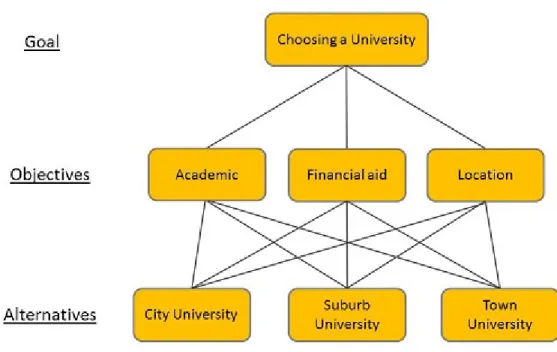
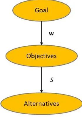
4.1 The Hierarchy for the Alice Example . . . 52
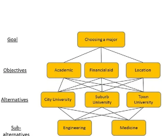
4.2 The Extended Hierarchy for the Alice Example . . . 54
6.1 Network for the Alice Example . . . 77
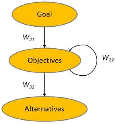
6.2 Network for a System with Feedback . . . 84
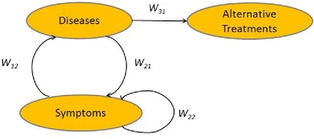
6.3 Network for the Case Study in Medical Diagnosis . . . 89
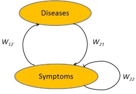
6.4 Reduced Network for the Case Study in Medical Diagnosis . . . . 95
6.5 Linear Network for the Case Study in Medical Diagnosis . . . 96
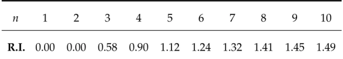
5.1 Values of the Random Index (R.I.) . . . 69
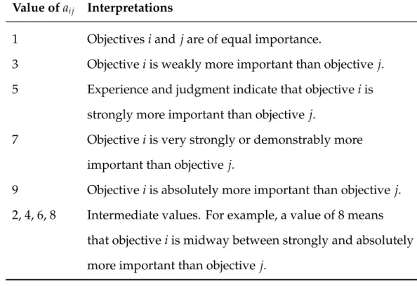
5.2 Interpretations of Entries in a Pairwise Comparison Matrix . . . . 73
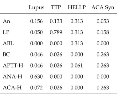
6.1 Priorities of Symptoms with Respect to Diseases . . . 100
6.2 Priorities of Diseases with Respect to Symptoms . . . 103
6.3 Priorities of Symptoms with Respect to Symptoms . . . 105
6.4 Priorities of Alternatives with Respect to Diseases . . . 110
Introduction
1.1
Motivation
We make decisions every day. High school graduates decide which college to attend. Moms make up their minds as to how much time they should let their children watch TV each day. Chefs choose the spices to use in dishes. The Federal Reserve makes judgments about its monetary policy. Decision making is a part of everyday life, whether it be a personal choice, a decision with global impact, or anything in between. Being able to make right decisions can have a tremendously positive impact on individuals’ lives.
However, making the right decision is often easier said than done. For starters, assuming that the decision makers are aware of their options, they need to identify their goals in choosing among these options. (As a simple example, consider a buyer, who is trying to decide between two kinds of tomatoes. He or she needs to know what qualities in tomatoes he or she values: the color, the shape, or the price.) Then, the decision makers need to
determine how well each option satisfies their goals. Even when the decision makers have clear ideas of their goals and the qualities of their options, their judgments can still exhibit inconsistency, or can vary according to time. Variations can also occur due to the environment that surrounds the decision making process.
The Analytic Hierarchy Process (AHP), developed by Thomas Saaty [10] is a model that helps the decision makers arrive at the most logical choice. Using the AHP, we first determine the options available to the decision makers and their goals in making decisions. These goals and options will then be used to construct an analytic hierarchy, which reflects the various factors in the decision making process and their importance. The outcome of the AHP is a priority vector, which gives us an insight into the best option for the decision makers. In order to understand the strengths of the AHP, in the next section, we consider a simple problem of choosing universities.
1.2
The Initial Problem
Alice is in her last year of high school. She has been accepted to three major universities and is trying to decide which one to attend. Those universities are City University, Suburb University, and Town University. In evaluating a university, Alice considers three factors: the academic quality of the university, the financial aid package that the university offers her, and the quality of the town or city that surrounds the university. In our discussion of the AHP, we will refer to the universities that extend their acceptance to Alice as
One solution to Alice’s problem is to directly assess her opinion of each university. For example, Alice can assign a score to each university, on a scale of 1–10, based on each of her objectives. Then the total score of each university is the sum of the scores of that university on the three objectives. The
university with the highest total score is the one that Alice should attend. The solution to the problem seems easy enough.
However, what will happen if Alice has ten, instead of three, objectives? Then scoring the universities will be a more complicated and error-prone task. How about the possibility that each objective has a different level of
importance to Alice? Then we have to take into account not only the score of each university on each objective, but also the weight of each objective to Alice’s decision. The problem quickly escalates in terms of complexity if Alice also has different potential majors in mind, and her choice of university affects her choice of major. For example, one of the universities might not have a Pre-Health program, but it has a strong Music department (assuming that Alice is considering studying Pre-Health and Music). Another university has a prestigious Pre-Health curriculum, but it does not have a Music major. The third university has both Pre-Health and Music, allowing Alice more opportunities to explore her interest, but both of the programs are only average.
The AHP provides a systematic method of solving problems such as the one that Alice is facing. We mentioned in the last section that in order to apply the AHP, we first identify clearly the objectives and alternatives available to the decision makers. Then there are two steps that we need to carry out. First, we measure the importance of each objective to the decision maker, compared
to the importance of the other objectives. This relative importance is called the
weightof the objective. For ease of computing, we require that the measured
weights sum to 1 [4, p. 30]. For this example, suppose that the AHP has found the weights for academic quality, financial aid, and quality of location to be 0.6, 0.3, and 0.1, respectively. According to these weights, Alice considers the quality of a university’s education the most important factor in making her decision. Following in importance are the financial aid package that she is offered, and then the quality of the university’s location.
In the next step, the AHP measures how well each of the decision maker’s alternatives satisfies each of the objectives. The extent to which each
alternative meets the decision maker’s expectation in each objective is measured as a numerical value. This value is referred to as thescoreof the alternative on that objective. In this example, suppose that the AHP has found the scores for one of the universities, City University, on academic quality, financial aid, and quality of location, to be 5, 7.5, and 10, respectively. These scores indicate that Alice loves the setting of City University, while the
financial aid that she is offered is moderately good, and the academic quality is only average. We noted earlier that a decision maker’s preferences can exhibit inconsistency. The scores found by the AHP are not simply the decision maker’s assessment of his or her own preferences. The AHP achieves these scores using a systematic approach that will be discussed in Chapter 4, helping the decision maker make the most logical choice given his or her preferences.
The reader might have guessed that in order for Alice to make a decision, both the weights of her objectives and the score of each alternative on those objectives must be taken into account. Indeed, we utilize both kinds of
information to compute the total score for each alternative. For the first alternative, City University, we first take the products of each of City
University’s scores on an objective and the weight of that objective. Taking the sum of those products will give us the total score of City University. Using the values in this example, the total score of City University is computed as
follows:
5×0.6+7.5×0.3+10×0.1=6.25.
Given that we also know the score of the other alternatives on Alice’s
objectives, we can compute the total score of those alternatives using the same method explained above. The alternative with the highest total score should be chosen.
In subsequent chapters, it will be clear that the AHP involves more than just finding the weights of the objectives and the scores of the alternatives. In fact, the two steps outlined above are merely part of a hierarchy that is used to model the decision makers’ preferences. The same idea of a hierarchy that is used to solve Alice’s problem could be used to answer questions about
promotion and tenure in higher education [10, p. 162], the optimum choice of coal plants [10, p. 156], and measuring the world influence of nations such as the U.S., China, France, the U.K., Japan,. . .[10, p. 40]. For the purpose of understanding the foundations of the AHP, the next three chapters will investigate the two outlined tasks: finding the weights of the objectives and the scores of the alternatives. The discussion of the hierarchy will soon follow.
At this stage, the AHP problem is summarized in mathematical notations as follows: Suppose a decision maker hasnobjectives andmalternatives. In
the first step of the AHP, for theithobjective, the AHP generates a weightwi. In the second step, for theithobjective and thekthalternative, the AHP obtains a scoresikof thekthalternative on theith objective. The total score of thekth alternative is then computed by the following formula:
n
X
i=1
wisik. (1.1)
After the total scores of all alternatives have been calculated, the decision maker should choose the alternative that has the highest total score.
1.3
Research Outline
This thesis focuses on the method and mathematical reasoning of the AHP. The next two chapters cover the task of finding the weights of the objectives. Specifically, in Chapter 2, we will develop Alice’s problem, introducing the basic terms and concepts of the AHP. As will be clear in this chapter, an essential concept of the AHP is the consistency of the decision maker’s preferences. We will include the definition of consistency, and then focus on the consistent decision maker. In Chapter 3, we investigate the case of an inconsistent decision maker. We turn our attention to finding the scores of the alternatives in Chapter 4. The discussion of the scores naturally leads to the idea of a hierarchy. Having discussed the hierarchy, we apply it to extend our Alice’s problem. In Chapter 5, we examine some measurement issues of the AHP. Specifically, we will provide an explanation for the measure of the decision maker’s consistency, and comment on the scale that is used to
measure the decision maker’s pairwise preferences.
In the second-to-last chapter, we present a more sophisticated application of the AHP in medical diagnosis. The application in turn illustrates the Analytic Network Process, a generalization of the AHP to systems with dependence and feedback. Included in Chapter 7 are final remarks and ideas for future research.
The terminologies of the AHP are defined as they are first used in the subsequent chapters. Unless otherwise noted, these definitions apply throughout the thesis.
The Consistent Decision Maker
2.1
The Eigenvalue Problem
In this chapter, we tackle the first task of the AHP: finding the weight of each objective of the decision maker. We continue with the Alice example presented in the last chapter, introducing terms and concepts that are fundamental to the AHP. One such concept is what is called the pairwise comparison matrix. This concept will naturally lead to the idea of the decision maker’s consistency in preferences. The AHP problem will then be divided into two sub-problems: one for the consistent and the other for the inconsistent decision maker. In the rest of the chapter, we present the method of finding the weight vector for the consistent case. This method involves the eigenvalue problem, a concept central to the AHP. Finally, we provide an illustration of the eigenvalue problem for the Alice example.
It is the writer’s intention to start the discussion of the AHP with a simple, instructive example such as the problem of choosing university for Alice.
However, the AHP has a wide array of applications in more complicated situations. The complexity of these situations is enhanced by the fact that
(i) the decision maker has a large number of objectives, (ii) the objectives are divided into layers of importance,
(iii) there exists a relationship between objectives and alternatives, or any combination of those mentioned above. For more sophisticated applications of the AHP, the interested reader is referred to [10, p. 91–163], which covers topics such as prediction of the number of children in a household, designing the transport system for the Sudan, and the future of higher education in the United States.
In decision making problems that involve a large number of objectives, it is difficult to compare each objective to the rest of the objectives. The process tends to result in error, much like the process of scoring each alternative on a scale of 1–10, compared to the other alternatives, that we mentioned in the introduction. A method that provides a more accurate assessment of the available objectives is to compare the importance of each objective to that of
each otherobjective. This method results in thepairwise comparisons of objectives.
Returning to the Alice example, the AHP assumes that Alice knows the pairwise comparisons of her objectives. Suppose she values the quality of a university’s education twice as much as the financial aid that the university offers, and six times as much as the quality of the university’s location. Similarly, financial aid is three times as important to Alice as the quality of
location. These numerical values that represent the pairwise comparisons of objectives are placed into apairwise comparison matrixA:
A= 1 2 6 1 2 1 3 1 6 1 3 1 .
The entry in theithrow and the jth column of matrixAis the importance of objectiveicompared to that of objective j. For example,a13 =6 means that the
first objective, academic quality, is six times as important as the third objective, location. It follows that the entries in the diagonal of matrixAare equal to 1. Moreover, if objectiveiis twice as important as objective j, then objective j
must be half as important as objectivei. In other words,aji= a1i j. We also note that if Alice isconsistentin her preferences, thenai jajk=aik. That is, if she prefers academic quality twice as much as financial aid, and financial aid three times as much as location, then she must prefer academic quality six times as much as location to be considered a consistent decision maker. According to this definition, Alice in our example is consistent. However, a decision maker in real life is rarely consistent in her preferences. In Chapter 3, we will discuss the process of obtaining the weights of the objectives in the inconsistent case. It is in this inconsistent case that the mathematical reasoning becomes more complicated. For now, we turn our attention to the consistent case.
The next definitions formalize our discussion of the pairwise comparison matrix.
matrix for a decision maker withnobjectives is ann×nmatrixA=hai jisuch
that:
(i) ai j>0 fori,j=1, . . . ,n, and (ii) aji= a1i j fori,j=1, . . . ,n.
A matrixAthat satisfies condition (i) is defined to be apositivematrix. If
Asatisfies condition (ii), then it is said to be areciprocalmatrix. In the next chapters, when we refer to the pairwise comparison matrix of a decision maker, the assumption is that the matrix is positive and reciprocal. Also note that conditions (i) and (ii) in Definition 2.1 imply thataii=1 fori=1, . . . ,n.
Definition 2.2(Pairwise Comparison Matrix of a Consistent Decision Maker).
If a decision maker is consistent, then the pairwise comparison matrixA
satisfies the conditions in Definition 2.1, and (iii) aik=ai jajk fori,j,k=1, . . . ,n.
Recall that theai jentry inArepresents the importance of objectivei, compared to that of objective j. Letwi be the (unknown for the time being) weight of objectivei. We assume each of the weights is positive, and the weights sum to 1. Then for aconsistentdecision maker, thei jentry ofAcan be written as:
ai j =
wi
wj
.
We note that the above equality is guaranteed to be true only if the decision maker is consistent. Thus, we have an alternative definition of the pairwise comparison matrix for a consistent decision maker:
Definition 2.3. The pairwise comparison matrixAof a consistent decision maker has the following form:
A=hai j i = w1 w1 w1 w2 · · · w1 wn w2 w1 w2 w2 · · · w2 wn ... ... ... ... wn w1 wn w2 · · · wn wn , wherewi >0 and Pn i=1wi =1.
Definition 2.3 leads to the formal definition of theweight vectorof the decision maker:
Definition 2.4. The weight vectorwof a decision maker is of the form:
w=[wi]=
w1 w2 · · · wn
T
,
wherewi >0 andPni=1wi =1. The weight vectorwis also referred to as the
priority vectorof the decision maker.
As mentioned in the introduction, the goal of the AHP is to findw. The next theorem guarantees that for a consistent decision maker, we can always obtain this weight vector from the pairwise comparison matrixA.
Theorem 2.1. Suppose a decision maker is consistent and has n objectives. Let A be
the corresponding pairwise comparison matrix, andwthe weight vector. Thenwis an eigenvector of A with corresponding eigenvalueλ=n.
Proof. By Definition 2.3 and Definition 2.4 Aw= w1 w1 w1 w2 · · · w1 wn w2 w1 w2 w2 · · · w2 wn ... ... ... ... wn w1 wn w2 · · · wn wn w1 w2 ... wn = w1 w1w1+ w1 w2w2+ · · ·+ w1 wnwn w2 w1w1+ w2 w2w2+ · · ·+ w2 wnwn ... wn w1w1+ wn w2w2+ · · ·+ wn wnwn = nw1 nw2 ... nwn =n w1 w2 ... wn =nw.
Thus,wis an eigenvector ofAwith corresponding eigenvaluen.
From Theorem 2.1, we have a way to obtain the weight for each objective, given that we know the number of objectivesnand the pairwise comparison matrixA. We know this by observing that:
Aw=nw
⇔Aw−nw=0 ⇔Aw−nIw=0 ⇔(A−nI)w=0.
Thus,wis in null(A−nI), whereIis the identity matrix of an appropriate
The equation
Aw=nw (2.1)
proved in Theorem 2.1 is critical to the AHP. In Chapter 3, we will discuss certain conditions that allow us to apply Equation 2.1 to solve the decision making problem when the decision maker is inconsistent. In Chapter 5, this equation is once again important to our discussion of the decision maker’s consistency. Throughout the rest of this thesis, we shall refer to Equation 2.1 as
theeigenvalue problem.
The purpose of this section has been to present the eigenvalue problem in Equation 2.1. We close the section by the next theorem, which provides a quick and easy way to identify the weight vector when the decision maker is
consistent.
Theorem 2.2. The normalized form of any column of the matrix A=
wi
wj
is a solution to the eigenvalue problem Aw=nw, wherew=
w1 w2 · · · wn
T
is the weight vector solution and n is the number of objectives.
Proof. By Definition 2.3, the jcolumn ofAhas the form
w1 wj w2 wj · · · wn wj T ,
for j=1,2, . . . ,n. Therefore, each column ofAis simply a constant multiple of
w. It follows that the normalized form of any column ofAis a solution to the
eigenvalue problem.
weights of Alice’s objectives. Our expectation is that the methods from both theorems give the same weight vectors.
2.2
Finding the Weight Vector for the Alice
Example
In this section, we illustrate the process of finding the weight vectors for the Alice example, using both Theorem 2.1 and Theorem 2.2. By our definition of consistent pairwise comparison matrices, the matrixAin the Alice example, which was given in the last section, is consistent. This guarantees that we can apply both theorems to obtain the weight vectors to solve Alice’s problem.
First, applying Theorem 2.1, we know thatλ =3 is an eigenvalue ofAand thatwis in the null space ofA−3I. In order to find the solutions of the
homogeneous system (A−3I)w=0, we first find:
A−nI =A−3I = 1 2 6 1 2 1 3 1 6 1 3 1 − 3 0 0 0 3 0 0 0 3 = −2 2 6 1 2 −2 3 1 6 1 3 −2 .
The reduced row echelon form ofA−3Iis:
1 0 −6 0 1 −3 0 0 0 . Using
Gauss-Jordan elimination [8, p. 78], the eigenvectors ofAwith corresponding eigenvalue 3 have the form
6s 3s s
T
(s∈R).
eigenvalue 3 is
6 3 1
T
.Since the weights of all of the objectives sum to 1, the weight vector is
w= 6 10 3 10 1 10 T .
According to this weight vector, the weights of the three objectives—academic quality, financial aid, and location—are 0.6, 0.3, and 0.1, respectively. This weight vector is indeed a constant multiple of any of the columns inA. So the methods of Theorem 2.1 and Theorem 2.2 yield the same result.
In this chapter, we have discussed the components essential to the
theoretical reasoning of the AHP. The discussion of the pairwise comparison matrix at the beginning of the chapter brought about the bifurcation of the AHP problem into the consistent and the inconsistent sub-problems. We also justified the existence of a solution to the AHP in the consistent case by the eigenvalue problem. In the next chapter, we shall see how this problem is utilized in solving for the weight vector in the inconsistent case.
The Inconsistent Decision Maker
3.1
From Consistent to Inconsistent
In reality, decision makers are usually inconsistent. For example, if a prospective college student prefers academic quality twice as much as financial aid, and financial aid three times as much as location, it is unlikely that she will prefer academic quality six times as much as location. As a result, for then×npairwise comparison matrixA=hai ji, it no longer holds that
aik=ai jajkfori, j,k=1, . . . ,n. Therefore, we cannot directly apply the
eigenvalue problem presented in the last chapter to the inconsistent case. (We note thatAis still a positive, reciprocal matrix. This means thatai j >0 and
ai j = a1ji for alliand j.)
Saaty contends that if the entries of a positive reciprocal matrix change by small amounts, then the eigenvalues of that matrix also change by small amounts [10, p. 51]. In addition, the corresponding eigenvectors do not vary by much. Provided that our decision maker is not too inconsistent, the
inconsistent pairwise comparison matrix will not deviate much from the consistent matrix. We can find the weight vector for an inconsistent decision maker based on the weight vector in theconsistentcase. Thus, we want to further explore the eigenvalues and corresponding eigenvectors of a consistent pairwise matrix. The next theorem serves that purpose.
Theorem 3.1. Suppose a decision maker is consistent and has n objectives. Then the
pairwise comparison matrix has a unique largest eigenvalue n. All of the other eigenvalues are zero.
Proof. In the last chapter, we proved that
Aw=nw.
Sowis an eigenvector ofAwith corresponding eigenvalueλ =n. Consider: A w1 0 ... 0 −wn = w1 w1 w1 w2 · · · w1 wn w2 w1 w2 w2 · · · w2 wn ... ... · · · ... wn−1 w1 wn−1 w2 · · · wn−1 wn wn w1 wn w2 · · · wn wn w1 0 ... 0 −wn = w1−w1 w2−w2 ... wn−1−wn−1 wn−wn = 0 0 ... 0 0 =0 w1 0 ... 0 −wn .
Thus, the vector w1 0 ... 0 −wn
is an eigenvector ofAwith corresponding eigenvalue
λ=0. Using the same approach, we can prove that the following vectors are the eigenvectors corresponding to the eigenvalueλ=0 forA:
w1 0 0 ... 0 −wn , 0 w2 0 ... 0 −wn , 0 0 w3 ... 0 −wn , . . . , 0 0 0 ... wn−1 −wn . | {z } n-1vectors
It can be easily seen that thesen−1 vectors are linearly independent, since
none of them could be written as a linear combination of the others. So the basis of the eigenspace associated with the eigenvalueλ=0 has at leastn−1
vectors. In other words, the geometric multiplicity of the eigenvalueλ=0, which is the dimension of the eigenspace associated with that eigenvalue, is at leastn−1. Since the algebraic multiplicity of the eigenvalueλ =0, which is
the number of times its factor occurs in the characteristic polynomial, is always bigger than or equal to its geometric multiplicity, the factor of the eigenvalue 0 occurs at leastn−1 times in the characteristic polynomial.
2.1, we already proved thatλ=nis an eigenvalue ofA. Therefore, the factor of the eigenvalueλ=0 can only occur in the characteristic polynomialn−1
times, since the factor of the eigenvalueλ =nhas to occur at least once in the characteristic polynomial with degreen. Therefore, the characteristic
polynomial ofAisp(λ)=λn−1
(λ−n).
Thus, the matrixAhas a unique largest eigenvalueλ=nand all of the
other eigenvalues equal zero.
From the proof above, when the eigenvalue ofAis 0, the corresponding eigenvectors violate the assumptionwi >0. Therefore, the only useful eigenvalue ofAisλ=n. Provided that the decision maker is slightly inconsistent, we expect thatAhas a unique largest eigenvalue that
approximatesn. The corresponding eigenvector, denotedw0, approximatesw.
Our problem for the inconsistent case becomes: given a decision maker that is inconsistent in her preferences, find the weight vectorw0that satisfies
Aw0 =λmaxw0, (3.1)
whereλmaxis the unique largest eigenvalue forA. In Section 3.2, we will discuss Perron’s theorem, which guarantees that Equation 3.1 always has a unique solution.
3.2
Positive Matrices and Their Eigenvalues
In this section, we discuss Perron’s theorem for positive matrices. The proof of this theorem provides the theoretical foundation for the method of finding the
weight vector in the inconsistent case. We begin by introducing several concepts and theorems about stochastic matrices. These results will be useful for our proof of Perron’s theorem later. The statement and the proof of
Perron’s theorem are presented in the second half of the section. The idea of the proof of Perron’s theorem in this section draws from an outline provided by Saaty [10, p. 170–176].
In Chapter 2, we mentioned the condition that makes a matrix positive. For the purpose of the theorems in this section, we provide a formal definition of the termsnon-negative matrixandpositive matrix.
Definition 3.1. A real matrixAis non-negative (or positive) if all of the entries
ofAare non-negative (or positive). We writeA≥0 (orA>0).
Definition 3.2. A non-negative matrixMis a stochastic matrix if each of the
row sums equal 1 [16, p. 189].
In another common definition of stochastic matrix, the entries in each of the columns ofMsum to 1. We can also say that the columns ofMare probability vectors. An example of a column stochastic matrix isM=
0.7 0.2 0.3 0.8 .
Theorem 3.2. For a positive, n×n, row stochastic matrix M
lim k→∞M k =ev, wherev= v1 v2 · · · vn
is a positive row vector,Pn
i=1vi =1, and e= 1 1 · · · 1 T .
Proof. Theorem 3.2 states that for largek,Mk approaches a matrix with identical rows. In order to prove this theorem, we prove that each column of
Mk approaches a column vector with identical entries. Let
y0 = y1 0 y 2 0 · · · y n 0 T
be an arbitrary column vector inRn. Define
yk =Mky0, withk=0,1,2, . . .. Letak andbkbe the maximum and minimum components ofyk, respectively. Further, letαbe the minimum entry inM.
The outline of the proof is as follows: (i) first, we demonstrate that the sequences (ak) and (bk) are monotone, and (ii) bounded. As a result, (ak) and (bk) converge. (iii) Next, we prove that the difference between (ak) and (bk) approaches 0 askapproaches infinity. Therefore, (ak) and (bk) tend to a
common limit, and all of the components inyk also approach this limit. Soyk
approaches a column vector with identical entries. (iv) Lastly, we choosey0so
that for eachy0,yk represent a column ofMk. Putting everything together,
each column ofMk approaches a column vector whose entries are the same, andMkapproaches a matrix whose rows are identical.
(i) The sequences(ak)and(bk)are monotone:
We observe that fork=0,1,2, . . .,yk+1 =Mk+1y0 =MMky0=Myk. Let yi
k+1be thei
thcomponent ofy
k+1, ykj be the jthcomponent ofyk, andmi,jbe the entry in theithrow and jthcolumn ofM, we have
yik+1 =
n
X
j=1
mi,jykj =mi,1y1k +mi,2y2k+. . .+mi,nynk. (3.2)
Without loss of generality, assume thaty1
yk. Then y1k =ak. Equation 3.2 could be rewritten as
yik+1 =mi,1ak+mi,2y2k+. . .+mi,nynk.
Sincebk is the minimum component ofyk,
yik+1 =mi,1ak+mi,2y2k +. . .+mi,nynk
≥mi,1ak+mi,2bk+. . .+mi,nbk
=mi,1ak+(1−mi,1)bk.
The last line was achieved because the entries in each row ofMsum to unity. Further, sinceαis the minimum entry inM,α≤mi,1and
1−α≥1−mi,1. Therefore
yik+1 ≥mi,1ak+(1−mi,1)bk ≥αak+(1−α)bk.
Similarly, without loss of generality, assume that y2k is the minimum component ofyk. Then y2k =bk. Equation 3.2 could be rewritten as
With the same reasoning as the case above, we could write
yik+1 =mi,1y1k+mi,2bk+. . .+mi,nynk
≤mi,1ak+mi,2bk+. . .+mi,nak
=mi,2bk+(1−mi,2)ak
≤αbk+(1−α)ak.
We just showed that an arbitrary component ofyk+1has the following
bounds:
αak+(1−α)bk ≤ yik+1 ≤αbk+(1−α)ak. (3.3)
Since the bounds hold for the largest component ofyk+1
ak+1 ≤αbk+(1−α)ak, (3.4)
which is equivalent to
ak+1−ak ≤α(bk−ak).
Becausebk ≤ak fork=0,1,2, . . .
ak+1−ak ≤α(bk −ak)≤0
fork=0,1,2, . . .. Thus, (ak) is decreasing.
yk+1. As a result
bk+1 ≥αak+(1−α)bk, (3.5) which is equivalent to
bk+1−bk ≥α(ak−bk)≥0,
for allk=0,1,2, . . .. Thus, (bk) is increasing.
(ii) The sequences(ak)and(bk)are bounded and convergent:
We showed that (ak) is decreasing and (bk) is increasing. Thus, for
k=0,1,2, . . .,ak ≤a0andbk ≥b0.
Fork=0,1,2, . . .,bk ≤ak ≤a0. Thus, the increasing sequence (bk) is
bounded above by the numbera0.
Similarly, fork=0,1,2, . . .,ak ≥bk ≥b0. Therefore, the decreasing
sequence (ak) is bounded below by the numberb0.
By the Monotone Convergence Theorem [1, p. 51], since (ak) is monotone and bounded, it converges. Likewise, (bk) converges.
(iii) The vector ykapproaches a column vector with identical entries:
Combining Equation 3.4 and Equation 3.5, we have
which is equivalent to
ak+1−bk+1 ≤(1−2α)(ak−bk). (3.6)
Next, we prove that (ak−bk)≤(1−2α)k(a0−b0) by induction.
Choosingk=0 and applying Equation 3.6, we have
a1−b1 ≤(1−2α)1(a0−b0),
so the base case is satisfied.
Assumean−bn ≤(1−2α)n(a0−b0). Then by Equation 3.6
an+1−bn+1 ≤(1−2α)(an−bn).
By our assumption of the induction hypothesis, the quantity on the left-hand side of the above inequality is less than or equal to
(1−2α)(1−2α)n(a0−b0). Thus
an+1−bn+1 ≤(1−2α)n+1(a0−b0).
By induction,
ak−bk ≤(1−2α)k(a0−b0). (3.7)
We showed that (ak) and (bk) converge. Therefore, the Algebraic Limit Theorem [1, p. 45] implies that (ak−bk) also converges. Next, we compute the limit of (ak−bk).
SinceMis a positive matrix whose row sums are ones, 0 < α <1. Thus
0<2α <2⇔ −1<1−2α <1⇔ |1−2α|<1,
which means limk→∞(1−2α)k =0 [1, p. 56].
From Equation 3.7 and the way we definedakandbk, we have
0≤ak−bk ≤(1−2α)k(a0−b0).
We knowlimk→∞0=0 and
limk→∞((1−2α)k(a0−b0))=(a0−b0) limk→∞((1−2α)k)=(a0−b0)0=0.
Using the Squeeze Theorem [1, p. 49], limk→∞(ak−bk)=0.
We showed that lim(ak) and lim(bk) exist. Again, by the Algebraic Limit Theorem lim k→∞(ak −bk)=0= lim k→∞(ak) −lim k→∞(bk).
Thus, (ak) and (bk) approach a common limit. Sinceakandbk are the maximum and minimum components ofyk, respectively, all of the
components inykalso approach this limit. In other words, ask
approaches infinity, the vectoryk approaches a column vector whose
entries are all the same. Since the decreasing sequence (ak) is bounded below byb0and the increasing sequence (bk) is bounded above bya0,
whereb0 ≤C≤a0ande=
1 1 · · · 1
T
.
(iv) Mkapproaches a matrix with identical rows:
Lety0= y1 0 y 2 0 · · · y n 0 T , with yi 0=1 andy j
0 =0 for any j,i. Then
yk =Mky0is theithcolumn ofMk.
We showed that askapproaches infinity, the vectorykapproaches a
column vector with identical entries. Therefore, theithcolumn ofMk also approaches a column vector with identical entries, askapproaches infinity.
LetCe=
ci ci · · · ci
T
. Sinceciis an entry inMk andMis positive,ci is also positive. Letvbe a row vector such thatvj =ci, we have
lim k→∞M k = c1 c2 · · · cn c1 c2 · · · cn ... ... ... c1 c2 · · · cn = 1 1 ... 1 c1 c2 · · · cn = 1 1 ... 1 v1 v2 · · · vn =ev.
Sinceci is positive,vis a positive row vector. The last item in the proof is to show that the sum of all of the components ofvis 1.
Since the rows ofMall sum to 1,Me=e, withe=
1 1 · · · 1
T
. We prove thatMk is also a stochastic matrix by induction.
First, sinceM1e=eas shown above, the base case is satisfied.
Assume thatMne=e. ThenMn+1e=M(Mne)=Me=e.
unity, and thereforePn
j=1vj =1.
We just proved that the powers of a positive, row stochastic matrix
eventually reach a stable stage. This result will be important to the proof of the next lemma, which is in turn useful for the proof of Perron’s theorem.
Lemma 3.1. If A is a positive n×n matrix, then
lim k→∞
Ak
λk =wv,
whereλis a positive constant,va positive row vector, andwis a positive column vector.
Proof. LetSbe the set of all non-negative, columnn-vectors such that the entries of each of those vectors sum to 1. We denote
S={x|x=[xi] n×1,xi ≥0, n X i=1 xi =1,i=1,2, . . . ,n}.
For any vectory, define the function
f(y)= n
X
i=1 yi,
and the matrix transformation
T(y)= 1
f(Ay)Ay, whereAis a positive,n×nmatrix.
The outline of the proof is as follows: (i) first, we demonstrate that the transformationTis a continuous function, andT(S)⊂S. That is for an
arbitraryx∈S,T(x)∈S. (ii) Next, using the Brouwer Fixed Point Theorem
with the functionTand the spaceS, we are able to find a positive fixed point w. (iii) Finally, we apply Theorem 3.2 to prove the proposed limit.
(i) Tis a continuous function which transformsStoS:
For an arbitraryx∈S, the matrix transformationAxis continuous, since
each component ofAxis a linear function ofx1,x2, . . . ,xnand therefore continuous. As a result,T(x) is continuous.
Let (Ax)ibe theithcomponent ofAx. Consider n X i=1 (T(x))i = n X i=1 ( 1 f(Ax)(Ax))i = f( 1 f(Ax)Ax) = (Ax)1 f(Ax) + (Ax)2 f(Ax) +. . .+ (Ax)n f(Ax) = 1 f(Ax) n X i=1 (Ax)i = 1 f(Ax)f(Ax) =1. SinceAisn×nandxisn×1,T(x) isn×1.
Further, sincex≥0 andPn
i=1xi =1,xhas at least one positive component. SinceAis positive,Ax>0, which leads to f(Ax)=Pn
i=1(Ax)i >0.
Therefore,T(x)>0.
To sum up, fori=1,2, . . . ,n,T(x)=[(T(x))i]n×1,T(x)>0,
Pn
Therefore,T(x)∈S.In other words,T: S→S.
(ii) Find w andλsuch thatAw=λw:
The spaceSis a closed boundedn−1 dimensional convex set inRn. ThusSis topologically equivalent to a closed disk inRn−1.
By the Brouwer Fixed Point Theorem [14, p. 277], there exists a fixed pointw∈Ssuch that
T(w)=w.
By our definition ofT, the above equation could be written as 1
f(Aw)Aw=w, (3.8)
which is equivalent to
Aw= f(Aw)w.
Likex,wis non-negative, with entries that sum to 1, sowhas at least one positive component. SoAw>0. Therefore, the right-hand side of the above equation has to be positive. Since we know thatwis non-negative,
f(Aw)>0 and thereforew>0.
Setλ= f(Aw). Then we have
Aw=λw, (3.9)
whereλis a positive real number andwis a positive columnn-vector. (iii) Proof of the proposed limit:
LetDbe a diagonal matrix,dii=wi anddi j =0 wheneveri, j(wi is theith component ofw). Then it follows thatw=De, withe=
1 1 · · · 1
T
.
For an arbitrary columnn-vectorz,Dz=0has only the trivial solution
z=0. Therefore,Dis invertible. D−1
is a diagonal matrix, with diagonal entries w1 i. It follows thatD −1 w=e. We observe that (D−1(1 λ)AD)e=(D −1 (1 λ)A)De=D −1 (1 λ)Aw=D −1 w=e. Thus,D−1
(λ1)ADis a row stochastic matrix. Further, sinceD−1
andDare non-negativen×nmatrices,Ais a positiven×nmatrix, andλis
positive,D−1
(λ1)ADis a positiven×nmatrix. Using Theorem 3.2,
lim k→∞(D −1 (1 λ)AD)k =ev ∗ , wherev∗=h v∗ i i 1×n >0, and Pn i=1v ∗ i =1.
On the other hand,
limk→∞(D −1 (1 λ)AD)k =klim→∞(D −1 (1 λ)AD)(D −1 (1 λ)AD). . .(D −1 (1 λ)AD) | {z } kterms ) =lim k→∞D −1 (1 λA)kD =D−1(lim k→∞ 1 λkA k)D.
Therefore, D−1(lim k→∞ 1 λkA k)D=ev∗ ⇔ lim k→∞ Ak λk =Dev ∗ D−1 =wv∗D−1. Letv=v∗ D−1 . Sincev∗
is a positive, rown-vector andD−1
is a non-negative,n×nmatrix,vis a positive rown-vector.
We have shown that for a positiven×nmatrixA,
lim k→∞
Ak
λk =wv,
whereλis a positive real number,va positive row vector, andwis a positive column vector.
We are now ready to state and prove Perron’s theorem, which justifies the existence of a unique largest eigenvalue and a corresponding eigenvectorw0
that satisfies Equation 3.1.
Theorem 3.3(Perron’s Theorem). Let A be a positive matrix. Then
1. A has a real positive simple (i.e., not multiple) eigenvalueλmax, whose modulus
is larger than the modulus of any other eigenvalues.
2. Each of the right and left eigenvectors of A corresponding to the eigenvalueλmax
has positive components, and is essentially (to within multiplication by a constant) unique.
3. The numberλmax(also called the Perron root of A) is bounded above by the
maximum row (or column) sum of A, and bounded below by the minimum row (or column) sum of A.
Proof. We claim that for a matrixA>0, the real numberλand the vectorsw andvconstructed in Lemma 3.1 satisfy Perron’s theorem. We present the proof in the following steps: (i) We first prove thatλis a eigenvalue ofAwith corresponding right eigenvectorwand left eigenvectorv, withλ,w, andv constructed in Lemma 3.1. (ii) Next, we prove thatλis the unique, largest eigenvalue ofA, which is the first item in Perron’s theorem. (iii) The proof that wandvare unique will be presented next. (iv) Lastly, we prove thatλis bounded above by the maximum row (or column) sum, and bounded below by the minimum row (or column) sum ofA.
(i) The real numberλis an eigenvalue ofAwith corresponding right
eigenvector w and left eigenvector v:
From Equation 3.9, we know thatλis an eigenvalue ofAwith corresponding right eigenvectorw.
Using the result of Lemma 3.1 1 λwvA= 1 λklim→∞ Ak λkA=klim→∞ Ak+1 λk+1 =wv. Therefore wvA=λwv, which is equivalent to ewvA=λewv,
in whiche=
1 1 · · · 1
is a rown-vector. Sinceewis a constant, we have
vA=λv, (3.10)
which means thatvis a left eigenvector ofAwith eigenvalueλ. We just showed thatwandvare the right and left eigenvectors ofA, respectively, with eigenvalueλ. The vectorswandv, as well asλ, are constructed in Lemma 3.1. In Lemma 3.1, we proved thatλis a positive real number,wis a positive column vector andvis a positive row vector.
(ii) The eigenvalueλis the unique, largest eigenvalue ofA:
Supposehis another eigenvalue ofAwith corresponding eigenvectoru.
ThenAu=hu. For any positive integerk,Aku=hku[8, p. 307]. This
means λ1kAku=(
h
λ)ku.
Taking the limit of both sides of the above equality and using the result of Lemma 3.1, we have: wvu=limk→∞(λh)ku.
Sincewvuis an columnn-vector, the limit on the right-hand side of the above equality has to exist, which means that limk→∞(λh)k has to exist.
Therefore,|h
λ|<1, which is equivalent to
|h|<|λ|,
in which case limk→∞(λh)k =0. Thus,λis the unique, largest eigenvalue of A.
unique to within multiplication by a constant:
We first prove thatwis unique to within multiplication by a constant. Supposeuis another right eigenvector ofAcorresponding to the eigenvalueλ. ThenAu=λu. For any positive integerk,Aku=λku[8, p. 307]. Therefore 1
λkAku=u.
Taking the limit of both sides of the above equality and using the result of Lemma 3.1, we have: limk→∞(1
λkAku)=limk→∞u⇔wvu=u. Sincevu
is a constant, we can seta=vu. Thus
aw=u.
Similarly, to prove that any other left eigenvector ofAcorresponding to
λis a constant multiple ofv, supposeyA=λy. ThenyAk =λky(for any
k∈Z,k>0)[8, p. 307]. Therefore 1
λkyAk =y, which meansyλ1kAk =y.
Taking the limit of both sides of the above equation and using the result of Lemma 3.1, we haveylimk→∞ A
k
λk =limk→∞y⇔ywv=y. Sinceywis a
constant, we can setc=yw. Thus
cv=y.
λis also called theprincipal eigenvalueofA, with corresponding
principal eigenvectors wandv. Up to this point, we have proved the
first two items in Perron’s theorem. What remains to be shown is the upper and lower bounds ofλ.
(iv) The eigenvalueλis bounded above by the maximum row (or column)
sum ofAand bounded below by the minimum row (or column) sum
ofA:
Lete=
1 1 · · · 1
T
be a columnn-vector. The row sums ofAare given by the components ofAe. LetMbe the maximum row sum andm
be the minimum row sum ofA. Then
me≤Ae≤Me. (3.11)
We proved thatvis a left eigenvector ofAwith corresponding eigenvalueλ. From Equation 3.10, we havevAe=λve.
In addition, from 3.11, we have
vme≤vAe≤vMe.
Therefore
vme≤λve≤vMe. (3.12)
Sinceveis a positive real number (we proved thatv>0), we can divide 3.12 byve, yielding:
m≤λ≤M.
Using similar techniques, we can prove thatλis bounded above by the maximum column sum and bounded below by the minimum column sum. This time, lete=
1 1 · · · 1
sums ofAare given by the components ofeA. LetNbe the maximum column sum andnbe the minimum column sum ofA. Then
en≤eA≤eN.
Using Equation 3.9, we haveeAw=eλw. Therefore,enw≤eλw≤eNw,
which is equivalent to
n≤λ≤N.
Perron’s theorem guarantees that in the inconsistent case, we can always find the weight vector from a positive, reciprocal pairwise comparison matrix
A. (Equation 3.1 has a unique solution). The next theorem provides the justification for the method of finding the weight vector.
Theorem 3.4.
lim k→∞
Ake
eTAke =w1,
where A>0,w1is its principal eigenvector corresponding to the maximum eigenvalueλ1, such that
Pn
i=1(w1)i =1.
For the proof of this theorem, the reader is referred to [10, p. 176]. Theorem 3.4 states that in order to compute the weight vector of an inconsistent
pairwise comparison matrix, we raise the matrix to an arbitrarily large power, and then divide the sum of each row by the sum of the entries in the matrix .
In the next section, we illustrate this method of finding the weight vector for an inconsistent decision maker.
3.3
Finding the Weight Vector for the Inconsistent
Alice Example
In this section, we illustrate the use of Theorem 3.4 with the inconsistent version of our Alice example. The consistent pairwise comparison matrixAis modified so that Alice is inconsistent in her preferences:
A= 1 2 5 1 2 1 3 1 5 1 3 1 .
Sincea12a23=6,5=a13,Ais not consistent. Fork =1:
A1e=Ae= 1 2 5 1 2 1 3 1 5 1 3 1 1 1 1 = 8 9 2 23 15 , eTA1e= 1 1 1 1 2 5 1 2 1 3 1 5 1 3 1 1 1 1 = 421 30 .
Applying Theorem 3.4 and approximating the result to five decimal places, the eigenvector is w1 = A 1e eTA1e = 30 421 8 9 2 23 15 = 0.57007 0.32066 0.10926 .
Replicating this process for larger values ofkyields: w2 = A 2e eTA2e = 0.58176 0.30896 0.10928 w3 = A 3e eTA3e = 0.58157 0.30898 0.10945 w4 = A 4e eTA4e = 0.58155 0.30900 0.10945 w5= A 5e eTA5e = 0.58155 0.30900 0.10945 .
The values of the eigenvector have stabilized after five iterations. In general, we stop when
kwi−wi+1k< ,
where >0 is predetermined. The weights of Alice’s objectives are the entries ofw5: the weight of the first objective is the first entry ofw5, the weight of the second objective is the second entry, and so on. Fromw5, we can see that the
weights of academic quality, financial aid, and location are 0.58155,0.30900, and 0.10945, respectively. These weights are close to the weights in the
consistent case, which were found in Chapter 2 to be 0.6,0.3 and 0.1. This indicates that Alice is not too inconsistent in her preferences. The method to measure the degree of inconsistency will be presented in Chapter 5.
Up until now, we have explained the methods used to find the weight vectors in both the consistent and the inconsistent sub-problems of the AHP. If a decision maker is consistent, Equation 2.1 states that the desired weight vectorwis an eigenvector ofAwith corresponding eigenvaluen. By Theorem 2.2, we are assured thatwis simply the normalized form of any column inA.
If the decision maker is inconsistent, we find the largest eigenvector ofA
corresponding to the principal eigenvalueλmax. (In other words, we find a solution to Equation 3.1). Theorem 3.3 (Perron’s theorem) guarantees the existence of a unique solution to Equation 3.1. In order to find this unique principal eigenvector, we apply Theorem 3.4: raisingAto an arbitrarily large power, and then dividing each row sum by the sum of the entries in the matrix. The iterations are stopped when the difference between two resulting vectors is less than a prescribed value. Since the goal is for the resulting
vectors to converge, a quick way to obtain the weight vector is to raiseAto the 2·ipower at theiiteration, fori=1, . . . ,n[10, p. 179].
In the next chapter, we turn our attention to the second task of the AHP: finding how well each alternative satisfies each objective.
Finding the Score of an Alternative
on an Objective
In this chapter, we present the method to determine the score of each
alternative on each objective. After the scores have been obtained, we will be able to calculate the priority of each alternative. As it turns out, the method to compute the scores of the alternatives is by nature similar to the process used to obtain the weights of the objectives. This leads to the generalization of the AHP, which at its heart involves the construction of ahierarchywith different
levels(or strata) in order to model the various elements in a decision maker’s
preferences.
46 OBJECTIVE
4.1
Finding the Score of Each Alternative in the
Alice Example
The computation of the scores starts with the construction of a pairwise comparison matrix. In Chapter 2 and Chapter 3, the pairwise comparison matrix has been used to compare each pair of the objectives in terms of their importance to the goal. In this chapter, we construct a pairwise comparison matrix for each objective, assessing how well each alternative satisfies that objective, compared to each other alternative. In other words, we are now interested in thepairwise comparisons of alternativeson each objective.
Not surprisingly, we aim to obtain thescore vector son an objective from the pairwise comparison matrix for that objective. If the matrix is consistent, we apply Theorem 2.2 to finds. If the matrix is inconsistent, we findsby using Theorem 3.4. In a nutshell, finding the scores of the alternatives on an
objective uses the same process as finding the weights of the objectives on the decision maker’s final choice. The only difference is that we have to repeat this process for each objective. We illustrate this process with the Alice example.
Recall that Alice has been accepted into three universities: City University, Suburb University, and Town University. Suppose further that we know how well each university satisfies each objective, compared to how welleach other
university satisfies the same objective. The extent to which alternativei
satisfies an objective, compared to the extent to which alternative jsatisfies that same objective, is measured on an integer-valued, 1–9 scale.1 These
1This scale is the same scale that was used to measure the pairwise comparisons of objectives
pairwise comparative scores are placed into a pairwise comparison matrix for each objective. For example, for the first objective, academic quality, the pairwise comparison matrix comparing each pair of the three universities is
B1= 1 4 8 1 4 1 3 1 8 1 3 1 .
Thei jentry inB1reflects the score of universityion academic quality,
compared to the score of university jon the same objective. In this example, suppose we refer to City University, Suburb University, and Town University as the first, second, and third university, respectively. Then the entry in the second row and the first column ofB1, which is 14, means that Suburb
University scores one fourth as well as City University on academic quality.
ThoughB1is a positive, reciprocal matrix as required, it is inconsistent,
sinceb12b23=4·3=12,8=b13. Applying Theorem 3.4, we find the score
vectors1forB1: s11 = B 1 1e eTB1 1e = 0.69488 0.22717 0.07795 s21 = B 2 1e eTB2 1e = 0.71788 0.20459 0.07753
48 OBJECTIVE s31 = B 3 1e eTB3 1e = 0.71677 0.20496 0.07826 s41 = B 4 1e eTB4 1e = 0.71664 0.20509 0.07826 s51 = B 5 1e eTB5 1e = 0.71665 0.20509 0.07826 s61 = B 6 1e eTB6 1e = 0.71665 0.20509 0.07826 .
The values ofs1 are within our convergence tolerance=0.00001 after the
sixth iteration. The first entry of this vector is the score of the first alternative on the objective academic quality, the second entry corresponds to the score of the second alternative on that objective, and so on. Based ons61, we know that the scores of City University, Suburb University, and Town University on the objective academic quality are 0.71665,0.20509,and 0.07826, respectively. Note that just like the weights of the objectives, these