Durham Research Online
Deposited in DRO:02 October 2019
Version of attached le: Accepted Version
Peer-review status of attached le: Peer-reviewed
Citation for published item:
Ahmadini, A.A.H. and Coolen, F.P.A. (2019) 'Statistical inference for the Arrhenius-Weibull accelerated life testing model with imprecision based on the likelihood ratio test.', Proceedings of the institution of
mechanical engineers, part O : journal of risk and reliability. . Further information on publisher's website:
https://journals.sagepub.com/home/pio
Publisher's copyright statement: Additional information:
Use policy
The full-text may be used and/or reproduced, and given to third parties in any format or medium, without prior permission or charge, for personal research or study, educational, or not-for-prot purposes provided that:
• a full bibliographic reference is made to the original source
• alinkis made to the metadata record in DRO
• the full-text is not changed in any way
The full-text must not be sold in any format or medium without the formal permission of the copyright holders. Please consult thefull DRO policyfor further details.
Statistical inference for the Arrhenius-Weibull
accelerated life testing model with imprecision
based on the likelihood ratio test
Abdullah A.H. Ahmadini
Department of Mathematics, Faculty of Science, Jazan University, Jazan, Saudi Arabia Frank P.A. Coolen
Department of Mathematical Sciences, Durham University, Durham, United Kingdom
Abstract
In this paper, we present a new imprecise statistical inference method for accelerated life testing data, where nonparametric predictive inferences at normal stress levels are integrated with a parametric Arrhenius-Weibull model. The method includes imprecision based on the likelihood ratio test which provides robustness with regard to the model assumptions. We use the likelihood ratio test to obtain an interval for the parameter of the Arrhenius link function providing imprecision into the method. The imprecision leads to observations at increased stress levels being transformed into interval-valued observations at the normal stress level, where the width of an interval is larger for observations from higher stress levels. If the model fits well, our method has relatively little imprecision. However, if the model fits poorly, it leads to more imprecision. Simulation studies are presented to investigate the performance of the proposed method.
Keywords: Accelerated life testing, Arrhenius-Weibull model, failure data, imprecise probability, likelihood ratio test, lower and upper survival functions, nonparametric predictive inference
1. Introduction
Accelerated life testing (ALT) is frequently used to obtain information on the lifespan of devices. Testing items under normal conditions can require a great deal of time and expense. To determine the reliability of devices in a shorter period of time, and with lower costs, it may be possible to use ALT. In ALT, a unit is
5
tested under levels of physical stress (e.g. temperature, voltage, or pressure) greater than normal operating conditions. Using this method, devices will fail more quickly, enabling estimation of the lifetime under normal conditions via extrapolation using an ALT model. There is a wide range of designs for ALT, including constant-, step-and progressive-stress testing [23]. Two components usually used to extrapolate a
device’s lifespan under normal use conditions from ALT results are the life time distribution (e.g. Weibull or log-normal) and the relationship between failure time and stress level (e.g. Arrhenius law or power law).
In recent decades, various methods for analyzing ALT data and a variety of applications for assessing the reliability with different ALT scenarios have been
in-15
troduced. An excellent introduction to ALT was given by Nelson [23]. Since Nelson [23], there has been a large amount of literature on ALT and a variety of statistical methods have been devoloped, we mention several recent contributions. Fan et al. [14] developed the maximum likelihood estimation (MLE) and Bayesian inference on all parameters of ALT models under an exponential distribution, with a link
20
function between the failure rate and the stress variables in a linear way under the Box-Cox transformation. Fard and Li [15] presented optimal step stress to obtain the optimal hold time at which the stress level is changed for step stress ALT design for reliability prediction. They assumed a Weibull distribution for the failure time at any constant stress level, and the scale parameter of the Wiebull distribution
25
is assumed to be a log-linear function of the stress level. Elsayed and Zhang [13] proposed an optimal multiple-stress-type ALT plan using a proportional hazards model to obtain failure time data rapidly in a short period of time. Sha and Pan [27] introduced step-stress ALT with Bayesian analysis for the Weibull proportional hazard model. Nasir and Pan [22] posited a Bayesian optimal design criterion and
30
presented acceleration model selection ALT studies, while Han [16] conducted re-search into temporally and financially constrained constant-stress and step-stress ALT.
Whilst ALT models typically consider failure times as the events of interest, there have also been important contributions with more detailed modelling, in particular
35
exploiting methods to mathematically model degradation processes. For example, Liao and Tseng [19], proposed an optimal design for step-stress accelerated degra-dation tests with the degradegra-dation process modelled as a stochastic diffusion process. Pan et al. [25] presented a bivariate constant stress accelerated degradation model and related inference. They assumed a device which has two performance
charac-40
teristics which are controlled by a Wiener process, to determine the relibility of high quality devices with a time scale transformation, and the Frank copula is used to model dependence of the two performance characteristics. Duan and Wang [12] pro-posed a bivariate constant stress accelerated degradation model with inference based on the Inverse Gaussian Process. It is important to note here that the modelling of
45
degradation processes does require much information about the engineering process and physical properties of the equipment, which may come from detailed measure-ments of the process or expert judgemeasure-ments. While this is an important development for real world accelerated life testing, we do not address such approaches further in this paper and only assume information about the failure times to be present.
50
Yin et al. [29] introduced imprecise probability theory [4] for ALT data using the power-Weibull model. In this paper we follow the same approach used by Yin et al. [29] but we investigate the Arrhenius-Weibull model, so a different link function is
used between different stress levels. The methods are basically the same, but Yin et al. [29] did not give an argument, other than simulation studies, for the imprecision
55
in the parameter. We use a parametric statistical test between the pairwise stress levels, to obtain the intervals for the parameter of the link function for which we do not reject the null hypothesis. This use of a frequentist statistical test to determine the level of imprecision is the main novelty in this paper.
We develop a new likelihood ratio test based method for analysing ALT data
60
with imprecise probabilities, where nonparametric predictive inferences (NPI) at the normal stress level is integrated with a parametric Arrhenius-Weibull model. This new method consist of two steps. First, we assume the Arrhenius-Weibull model for all levels and we derive an interval for the parameter of the Arrhenius link function by pairwise likelihood ratio tests, which allows observations of increased
65
stress levels to be transformed to interval-valued observations at the normal stress level. Secondly, we use NPI at the normal stress level for predictive inference on the failure time of a future unit operating under normal stress, using the original data at the normal stress level and interval-valued data transformed from higher stress levels.
70
This paper is organized as follows: in Section 3, the main ideas of nonparametric predictive inference are briefly reviewed. In Section 4, our novel method of imprecise statistical inference is introduced. Section 5 presents an example with simulated data in order to illustrate our method and its main properties. In Section 6 the new method is applied to a data set from the literature. Section 7 presents results of
75
simulation studies that investigate the performance of the proposed method. Finally, some concluding remarks are made in Section 8.
2. The model
In this paper, we consider the Arrhenius model and a Weibull lifetime distribution for a constant-stress ALT. The Arrhenius model is based on physical or chemical
80
theory, and is often an appropriate model to use when the failure mechanism is driven by temperature [23]. The Weibull distribution is often suitable for examining component, system or product life. The Arrhenius-Weibull model is adopted to the current research on imprecise statistical approaches to establish the use of impreci-sion in modelling the nature of the relationship between stress levels and unit failure
85
rates. The main issue here is how to extrapolate the failure data from units tested at higher-than-normal stress levels to units operating at the normal stress level.
The model at each stress level (the two-parameter Weibull distribution) is f(t) = β αi ( t αi )β−1exp h −( t αi )β i . (1)
The unknown parameters of the Weibull distribution are the shape parameter β, and the scale parameters αi at stress level i, where αi > 0 and β > 0, and its
90
P(T > t) = exph− t αi
βi
.
The Arrhenius-Weibull model is specified as follows. K0 represents the stress at
the normal level. There are m ≥ 1 increased stress levels, with stress Ki at level
i ∈ {1, ..., m}, we assume that Ki increases as a function of i. In this paper, the Weibull distributions for different stress levels are assumed to have different scale
95
parametersαi >0 for level i, but the same shape parameter β. The Arrhenius link function for the scale parameters is
αi =α0exp γ Ki − γ K0 . (2)
Using this model with varying temperatures (in Kelvin) as stress levels, K0 is
the normal temperature at stress level 0,Ki is the higher temperature at stress level i, andγ >0 is the parameter of the Arrhenius link function model.
100
Using this link function model, an observation ti at the stress level i, subject
to stress Ki, can be transformed to stress level 0. For fixed γ the transformed
observation denoted by ti→0(γ) from level i to level 0 is given by the equation
ti→0(γ) = tiexp γ K0 − γ Ki . (3)
Now, we define the model through the probability density function as: f(ti;α, β, γ, K) = β αi ti→0(γ) αi β−1 exp − ti→0(γ) αi β! , (4)
where the Arrhenius link function for scale parameters αi should be identified to
105
establish a connection between the different stress levels i.
Let all the data be denoted by t
∼ = {t 0 1, ...t0n0, t 1 1, ...t1n1, ..., t m
1 , ...tmnm} and let the
stress levels be denoted byK ={K0, ..., Km}. The likelihood function is defined as L(t ∼;α, β, γ, K) = m Y j=0 nj Y i=1 f tji;α, β, γ, K.
So there are in total three parameters that need to be estimated to fit the com-plete model,α0,β, and γ. In this paper, we will apply the pairwise likelihood ratio
110
test to create an interval for the parameter γ of the link function, as presented in Section 4. We assume the same β for all stress levels, so differences between stress levels are only modelled through theαi, and hence in the model through theα0 and
γ parameters of the link function between different stress levels. For ease of
pre-sentation, we assume that there are no right-censored observations and that there
115
are failure observations at the normal stress level. We briefly comment on these assumptions in Section 8.
3. Nonparametric predictive inference
Nonparametric Predictive Inference (NPI) is a statistical method, which provides lower and upper survival functions for a future observation based on past data
120
using imprecise probability [4, 7]. Hill [17] proposed an assumption which gives direct conditional probabilities for a future random quantity which depend on the values of related random qualities [3, 6, 7]. It proposes that the rank of a future observation among the values already observed will be equally likely to have each possible value 1, ..., n+ 1. Suppose thatX1, X2, ..., Xn, Xn+1 represent exchangeable
125
and continuous real-valued possible random quanities, then the ranked observed values of X1, X2, ..., Xn can be denoted by x(1) < x(2) < ... < x(n). Let x0 = 0 and xn+1 =∞. The assumptionA(n) is
P(Xn+1 ∈(x(j−1), x(j))) = 1/(n+ 1).
Here, no tied observations are included for convenience, any tied values can be dealt with by assuming that tied observations differ by a small amount which tends
130
to zero [18].
Inferences which are based onA(n) are nonparametric and predictive. They can
be considered suitable if there is hardly any knowledge about the random quantity of interest, except for thenobservations, or if one does not want to use any such further information. TheA(n) assumption is not sufficient to derive precise probabilities for
135
many events of interest. However, this approach does yield optimal bounds for probabilities through the ’fundamental theorem of probability’ [11], which are lower and upper probabilities in the imprecise probability theory [3, 4].
The lower and upper probabilities for event A are denoted by P(A) and P(A), respectively. These are open to interpretation in various ways [4]. For instance,
140
P(A) can be assumed to be the supremum buying price for a gamble on event A,
such that ifA occurs then 1 is paid, if not then 0 is paid. This can also simply be interpreted as the maximum lower bound for the probability ofA, which derives from
the assumptions made. Similarly, P(A) can be interpreted as the minimum selling
price for the gamble onA, or the minimum upper bound based on the assumptions
145
made. We have 0 ≤ P(A) ≤ P(A) ≤ 1, and P(A) = 1−P(Ac) where, Ac is the
complimentary event of A [3, 4].
The NPI lower and upper survival functions for a future observation Xn+1 in
case of no censoring are SX n+1(t) = n−j n+ 1, for x∈(xj, xj+1), j = 0, ..., n. (5) SXn+1(t) = n+ 1−j n+ 1 , for x∈(xj, xj+1), j= 0, ..., n. (6) The imprecision, the difference between the upper and lower survival functions, reflects the amount of information in the data. We will only use Equations (5) and (6) for the NPI method in this paper.
4. ALT inference using pairwise likelihood ratio tests
To investigate equality of two independent failure data groups, possibly including right-censored observations, the likelihood ratio test can be used [26]. This is a popular statistical test that can be applied to investigate equality of the probability distribution of two independent groups, which has been briefly introduced in Section
155
1 [2, 23].
In this section we present new predictive inference based on ALT data and the likelihood ratio test. We use NPI at the normal stress level, with the fully parametric model used in our new statistical method analysing data from ALT. The use of NPI here provides lower and upper survival functions for a future observation at the
160
normal stress level, based on all failure data.
This new statistical method for data in ALT divides into two steps. First, the basic Arrhenius-Weibull model is adopted [23], and the pairwise likelihood ratio test is used between the stress levelsKi and stress levelK0, to obtain the intervals for the parameterγfor which we do not reject the null hypothesis that the data transformed
165
from stress level i to normal stress level 0, and the original data obtained at the
normal stress level 0, come from the same Weibull distribution. The hypothesis test we use in this paper is
(
H0 :γ =γ0 H1 :γ 6=γ0, whereγ ∈R. The test statistic is defined as
LR= L(t ∼; ˜α, ˜ β, γ0, K) L(t ∼; ˆα, ˆ β,ˆγ, K) where ˜α,β˜are such that sup(α,β)∈R+×
R+L(∼t;α, β, γ0, K) = L(∼t; ˜α,β, γ0, K˜ )
170
and ˆα,β,ˆ ˆγ are such that sup(α,β,γ)∈R+×
R+×RL(∼t;α, β, γ, K) =L(∼t; ˆα,β,ˆ ˆγ, K). The probability density function of the Arrhenius-Weibull model is assumed in this paper to describe the failure time at a fixed stress level, and its parameters are therefore maximized in the likelihood ratio test. There are in total three parameters that need to be estimated under the alternative hypothesis;α0,β, andγ. Under the
175
null hypothesis, for which γ is fixed whileα0 and β are estimated, theLR follows a χ12 distribution. To get [ γi,γi], for each value of γ we would have different ˆα0 and
ˆ
β but we do not use these any further in our method.
For each i = 1, ..., m, we find γ
i, the smallest value for γ0 for which we do not reject the null hypothesis, andγi, the largest value for γ0for which we do not reject
180
the null hypothesis. Then we define γ = max {min γ
i,0} and γ = max γi. Note that, because of the physical interpretation of generally faster failures with increased stress levels, we exclude negative values which leads to someγ values being set at 0.
In this paper, we will always restrict γ to non-negative values. We find the γ
i and
γi numerically using the statistical softwareR.
185
Note that, we do not make a confidence statement for the final NPI lower and upper survival functions, so we do not explicitly quantify the prediction accuracy. If indeed the main assumption is valid, that increased stress tends to decreased failure times, then negative γi are typically resulting from statistical variation and would disappear for larger samples.
190
One may wish to allowγ to be negative, which may e.g. be reasonable if it turned out that higher stress level could possibly improve a unit’s failure time. However, in normal ALT applications there tends to be sufficient knowledge about the effect of the stress on the failure times to justify negative values forγ not to be considered. Hence we also do not consider such values in this paper. It should be emphasized
195
though that our inferential method could still be used if negative values for lowerγ were allowed.
In the second step, we apply the data transformation using γ for all levels i =
1, ..., m to get transformed data at level 0, which are then used together with the original data at the normal stress level, to derive the NPI lower survival function
200
S. Similarly, we apply the data transformation using γ for all levels i = 1, ..., m to get transformed data at level 0, which are then used together with the original
data at the normal stress level, to derive the NPI upper survival function S. Note
that each observation at an increased stress level transforms into an interval-valued observation at the normal stress level 0, where the width of an interval is larger for
205
an observation from a higher stress level.
Note that, if the model fits really well, we expect most γ
i values to be quite
similar, as well as most γi values. If the model fits poorly, γ
i are most probably
very different, orγi are very different, or both. Hence, in case of poor model fit, the resulting interval [γ, γ] tends to be wider than in the case of good model fit. If the
210
model assumed is not too far from reality, we would expect the widest interval for
the parameter γ to come from the likelihood ratio test applied to levels 1 and 0.
If the model assumed is not too far from reality, we would expect the widest interval for the parameter γ to come from the likelihood ratio test applied to levels 1 and 0. If the model fits well, a level 1 observation is transformed to a smaller
215
interval on level 0 than a level 2 interval, if the transferred intervals are close, in
particular if they are overlapping. In the overlapping case, because the level 2
interval is wider, the left and right end points of these intervals from level 2 are
further apart, which implies that the γ in the null hypothesis will be rejected in
more cases. Hence, the interval [γ, γ] from level 1 will be wider than the interval
220
[γ, γ] from level 2 (in most cases, due to variability in the samples not in all cases).
If the model is worse than we would expect more often thatγ = γ
i for an i6= 1, or γ = γi for an i 6= 1. If the model assumptions are not fully correct, for example, using some misspecification cases or there is a lot of overlap between the data, then latter can happen.
225
com-bine these into a single test of a hypothesis involving all groups simultaneously. A multiple testing (comparison) procedure arises in many scenarios, where two groups of data are compared over time with each other [5, 24]. A well known scenario that one may be interested in testing is the comparison between two groups based
230
on confidence level [24]. While we use pairwise tests in our approach, we do not combine these into an overall confidence level statement for the resulting inference. Instead we use NPI to derive the lower and upper predictive survival functions and we investigate the performance of our predictive method separately via simulations.
If the assumed model is fully correct then the lower and upper γ will form an
235
interval with at least 1−α confidence level, with α the significance level for each pairwise test. However, we explicitly develop our method for robust inference as the basic assumed model will in practice not be ‘correct’, and acknowledging this makes confidence statements hard to justify. This is an interesting topic for future research. The method proposed in this section is illustrated by two examples using
240
simulated data and real data in Sections 5 and 6, and studied in more detailed by simulation in Section 7.
5. Example: simulated data
In this section we present an example consisting of two cases. In Case 1 we simulated data at all levels using the parametric model for the link function we
245
assume for the analysis. In Case 2 we change these data such that the assumed link function will not provide a good fit anymore and we investigate the effect on the interval [γ, γ] and the corresponding lower and upper predictive survival functions for the normal stress level. We assumed the normal temperature stress level to be
K0 = 283, and the increased temperatures stress levels K1 = 313 and K2 = 353
250
Kelvin. We generated ten observations from a Weibull distribution at each stress
level linked by the Arrhenius link function. The Weibull distribution at level K0
had shape parameter β = 3 and scale parameter α0 = 7000, and the Arrhenius
parameter was set atγ = 5200. This model keeps the same shape parameter at each
temperature, and the scale parameters are linked by the Arrhenius relation, which
255
led to α1 = 1202.942 at level K1 and α2 = 183.0914 at level K2. The ten failure times of units were simulated at each temperature, so data of a total of 30 units is used in the study. The failure times are given in Table 1.
To illustrate the pairwise likelihood ratio tests method using these data, we first assume the Weibul distribution at each stress level and the Arrhenius link function
260
for the data. To obtain the intervals [γ
i, γi] of the values γi for which we do not reject the null hypothesis with regard to the well-mixed data transformation, we used the pairwise likelihood ratio test betweenKi fori= 1,2 andK0. The resulting intervals [γ
i, γi] for three significance levels are given in Table 2.
In the second step of our method, we transformed the data using the [γ, γ]
265
values. All observations at the increased stress levels were transformed to the normal stress level. Therefore, the observations at the increased stress levels K1 and K2
Case K0 = 283 K1 = 313 K2 = 353 K1 = 313 (*1.4) K2 = 353 (*0.4) 1 2692.596 241.853 74.557 338.595 29.823 2 3208.336 759.562 94.983 1063.387 37.993 3 3324.788 769.321 138.003 1077.050 55.201 4 5218.419 832.807 180.090 1165.930 72.036 5 5417.057 867.770 180.670 1214.878 72.279 6 5759.910 1066.956 187.721 1493.739 75.088 7 6973.130 1185.382 200.828 1659.535 80.331 8 7690.554 1189.763 211.913 1665.668 84.765 9 8189.063 1401.084 233.529 1961.517 93.412 10 9847.477 1445.231 298.036 2023.323 119.214
Table 1: Failure times at three temperature levels in the first three columns and corresponding failure times with misspecification in the last two columns
Significance level 0.01 0.05 0.10 Stress level γi γi γi γi γi γi Case 1: K1 K0 4060.018 6605.752 4424.881 6261.168 4593.700 6100.653 K2 K0 4377.043 5602.321 4550.205 5434.908 4630.511 5357.037 Case 2: K1∗(1.4), K0 3066.539 5612.273 3431.402 5267.689 3600.221 5107.174 K2 ∗(0.4), K0 5684.708 6909.985 5857.870 6742.573 5938.175 6664.701
0 5000 10000 15000 20000 25000 30000 260 280 300 320 340 t0 y0
Figure 1: Some transformed data using [4060.018,6605.752]
are transformed to interval-valued observations at the normal stress level K0. We
briefly illustrate this in Figure 1 using only three points of the data at each level, therefore, we have six lines going down as shown in Figure 1. We transformed the
270
data from the higher stress levels K1 and K2 using [4060.018,6605.752] with 0.01 level of significance, mixed with the original samples at the normal stress levelK0.
Note that, in Figure 1 the two largest transformed data points are actually the γ
and γ transformations of the largest observation from level K2. So, this illustrates the key property of our method, that data transformed from higher levels tend to
275
be wider intervals at the normal level.
The NPI lower survival function is based on the original data at level 0 together with the transformed data from the stress levels K1 to K0 and K2 to K0 using γ. Similarly, the NPI upper survival function is based on the original data at level 0
together with the transformed data from the stress levels K1 to K0 and K2 to K0
280
using γ. The γ transformed the points to the smallest values and therefore is most
pessimistic case which leads to the lower survival functionS. Theγ transformed the points to the largest values and therefore is most optimistic case which leads to the upper survival function S. In Case 1, we take γ = 4060.018 and the γ = 6605.752, γ = 4424.881 andγ = 6261.168, andγ = 4593.700 andγ = 6100.653 of the pairwise
285
K1, K0 with 0.01, 0.05 and 0.10 significance levels, respectively. We used all the
aboveγ and γ values to transform the data to the normal stress level 0, see Figure
2(a). In this figure, the lower survival function S is labeled as S(γ
i) and the upper survival function S is labeled as S(γi). This figure shows that higher significance levels leads to more imprecision for the NPI lower and upper survival functions.
290
In Case 2, we illustrate our method in case of misspecification. We multiply the
data at level K1 by 1.4 and in addition we multiply the data at level K2 by 0.4.
case, we take γ = 3066.539 and γ = 6909.985, γ = 3431.402 and γ = 6742.573, and γ = 3600.221 and γ = 6664.701 for 0.01, 0.05 and 0.10 significance levels,
295
respectively. We used all the above γ and γ values to transform the data to the
normal stress level 0, see Figure 2(b). Figure 2(b) also shows that higher significance level results in more imprecision for the NPI lower and upper survival functions. In Case 2, we can see that the [γi, γi] intervals for the two pairwise comparisons are
fully disjoint unlike in Case 1. Note that in Case 2, the observations at level K1
300
have increased, leading to smaller γ
1 and γ1 values, which, in turn, leads to the
lower and upper survival functions to decrease in comparison to Case 1. Also, the observations at K2 stress level in Case 2 have decreased, resulting in larger values forγ
2 andγ2, and this leads to the lower and upper survival functions to increase in
comparison to Case 1. Therefore, it is obvious that considering the γ and γ values
305
give substantially more imprecision in our NPI method. In case of poor model fit, the NPI lower and upper survival functions in Figure 2(b), using our method as discussed in Section 4, have more imprecision than if the model fits well.
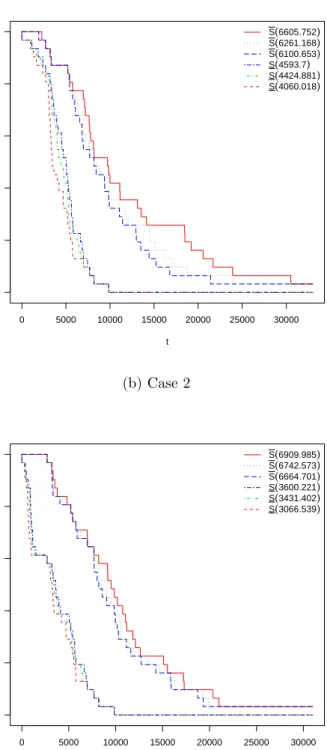
(a) Case 1 0 5000 10000 15000 20000 25000 30000 0.0 0.2 0.4 0.6 0.8 1.0 t Sur viv al function S(6605.752) S(6261.168) S(6100.653) S(4593.7) S(4424.881) S(4060.018) (b) Case 2 0 5000 10000 15000 20000 25000 30000 0.0 0.2 0.4 0.6 0.8 1.0 t Sur viv al function S(6909.985) S(6742.573) S(6664.701) S(3600.221) S(3431.402) S(3066.539)
Case K0 = 393 K0 = 408 K0 = 423 1 3850 3300 2750 2 4340 3720 3100 3 4760 4080 3400 4 5320 4560 3800 5 5740 4920 4100 6 6160 5280 4400 7 6580 5640 4700 8 7140 6120 5100 9 7980 6840 5700 10 8960 7680 6400
Table 3: Failure times at three temperature levels
Significance level 0.01 0.05 0.1 Stress level γ i γi γi γi γi γi K1 K0 0 4881.225 0 3988.558 0 3572.193 K2 K0 188.348 3540.639 651.091 3077.896 866.927 2862.060 Table 4: [γ
i, γi] for pairwise likelihood ratio tests.
6. Example: real data
The method proposed in Section 4 is now applied to a data set from the literature
310
[28], which result from a temperature-accelerated lifespan test. The time-to-failure
data were collected at three temperatures (in Kelvin): K0 = 393, K1 = 408, and
K2 = 423, with 393 the normal temperature for the process of interest. Ten units
were tested at each temperature, so a total of 30 units where used in the study. All of the units failed during the experiment. The failure times, in hours, are given in
315
Table 3.
For the data in Table 3, we have assumed the Weibull failure time distributions at each stress level, with the Arrhenius link function between different stress levels. Then the pairwise likelihood ratio test is used separately between levelKi and K0, for i = 1,2 to derive the intervals [γ
i, γi] for the value of the parameter γ of the
320
Arrhenius link function, such that we do not reject the null hypothesis that two
group of failure data (the transformed data from level i and the real data from
level 0) come from the same underlying distribution, is not rejected for values ofγ in this interval. The resulting intervals [γ
i, γi] are given in Table 4, for three test significance levels.
325
Note that, because the data corresponding to the different stress levels already have quite some overlap, the likelihood ratio tests even did not rule out some nega-tive values forγ. However, because of the physical interpretation of generally faster failures with increased temperature, we exclude negative values which leads to some
γ
i values being set at 0. Following the method presented in this paper, we
trans-330
formed the data using the overall values [γ, γ], derived as the smallest and largest corresponding values for the pairwise tests, respectively. Based on the original data at level 0 together with the data transformed from the stress levelsK1 toK0 andK2 toK0usingγ, the NPI approach provides the NPI lower survival function. Similarly,
but usingγ for the transformation, we derived the NPI upper survival function. For
335
the significance levels 0.01,0.05,0.1, the values ofγ are always 0 in this case, and for γ we have, 4881.225, 3988.558 and 3572.193, respectively. The resulting lower and upper survival functions are presented in Figure 3, where of course the three differ-ent significant levels lead to the same lower survival function due to the restriction for the γ values to be non-negative. In this figure, the lower survival function S is
340
labeled as S (γ
i) and the upper survival function S is labeled as S (γi). This figure shows that a smaller significance level leads to more imprecision for the NPI lower and upper survival functions, which is directly resulting from the fact that the inter-vals of not rejected values ofγi in the pairwise tests will be nested, becoming larger if the significance level is decreased. These lower and upper survival functions can
345
also be used to deduce corresponding lower and upper values for percentiles, which are found in the usual way by inverting the respective functions. These functions can also be used as inputs into decision processes, for example with regard to setting warranty policies, this is a topic of ongoing research by the authors.
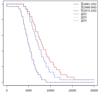
0 5000 10000 15000 20000 0.0 0.2 0.4 0.6 0.8 1.0 t Sur viv al function S(4881.225) S(3988.558) S(3572.193) S(0) S(0) S(0)
7. Simulation studies
350
The imprecise predictive statistical method we propose in this paper for ALT, uses the pairwise likelihood ratio tests with the parametric Arrhenius-Weibull model. This is intuitively attractive because it shows some robustness, and demonstrates the effect of imprecision when we lack perfect information about the link between different stress levels. In this section, we first apply simulation studies to investigate
355
the performance of our proposed method when considering the assumed Arrhenius-Weibull model as the true underlying model.
To investigate the predictive inference performance of our new method for ALT data, we conduct a simulation study. We assumed the temperature stress levels to
be K0 = 283, K1 = 313, and K2 = 353. In this analysis, we run the simulation
360
10,000 times with the data simulated from the Weibull distribution with β = 3, α
= 7000, and the Arrhenius link function parameter γ = 2000, where we have used
n = 10,50,100 assigned to each stress level. We applied the method described in
Section 4, with levels of significance 0.01, 0.05, and 0.10. For good performance of the method, we check the results by taking into account a future observation,
365
and we consider if it mixes well among the data at level K0, where we use both
the actual data at level K0 and the data transformed to level K0. We examined
the performance in the quartiles of NPI lower and upper survival functions for q= 0.25,0.50,0.75, and whether or not the future observation at the normal stress level has exceeded these quartiles in the right proportion. One can use different
370
quartiles but these quartiles provided a good indicator of the performance of our method. We conducted simulation with assumed Arrhenius-Weibull model, hence with data generated from the same model as used for our method, hence we expect a good performance.
For good performance of the method, we require that the future observation for
375
each run at the normal stress level has exceeded the first, second, and third quartiles of the NPI lower survival functions just over proportions 0.75,0.50 and 0.25 of all runs, respectively, and for the NPI upper survival functions just under proportions 0.75,0.50 and 0.25. Table 5 presents the results of the performance of our method for this simulation. All cases in Table 5 show an overall good performance of the
380
proposed method, with levels of significance 0.01,0.05, and 0.10, and with sample sizen = 10,50,100. Note that the quartiles in this table are denoted byqL andqU, corresponding to the NPI lower and upper survival functions, respectively. We note
that for corresponding proportion with larger values of n, the differences between
lower and upper survival functions tend to decrease. That means that when have
385
more data, the NPI lower and upper survival functions allow more precise infer-ence. As mentioned in Section 4, if the model fits very well or perfectly, then in
most cases γ = γ
1, and γ = γ1. Table 6 shows that when we simulate from the
assumed Arrhenius-Weibull model out of 10,000 runs with 0.05 level of significance, hence with data generated from the same model, that most of the widest intervals
390
ap-proach using the Arrhenius-Weibull model provides suitable predictive inference if the model assumptions are fully correct. We will investigate robustness in case of model misspecification in the next three simulation cases.
In Case 1, we are dealing with a particular misspecification of the model for
sta-395
tistical inference for ALT data [20, 21]. Table 7 presents the results of the predictive performance of our method. We used the same scenario as in the first simulation
but we assumed shape parameter β = 2 for each level, in the analysis. Now only
the scale parameterα and the parameter γ of the link function are explicitly
maxi-mize in the likelihood ratio. In comparison to the first simulation where the shape
400
parameter β = 3 was estimated, there is a slight effect on the quartiles in Table
7. From Table 5 and Table 7, the effect of fixing the shape parameter β = 2 in
the analysis can also be seen on the quartiles of the NPI lower and upper survival functions forq= 0.25,0.50,0.75, which is reflected by more imprecision for this case. Also, we checked whether or not the future observation at the normal stress level
405
has exceeded these quartiles in the right proportion. Further note that, in Table 7, there seems to be more imprecision than in Table 5. Throughout this simulation,
when we fixed the shape parameter β = 2 in the fitted model, our novel method
provided sufficient robustness against the misspecification.
In Case 2, we investigate the predictive performance of our method for ALT data
410
we change these data such that the assumed link function will not provide a good fit and we show the change to the resulting quartiles of NPI lower and upper survival functions for q = 0.25,0.50,0.75, and whether or not the future observation at the normal stress level has exceeded these quartiles in the right proportion.
To illustrate this, we generated data sets as before withn = 10,50,100
observa-415
tion at each stress level using the Arrhenius-Weibull model. But now all the data at stress levelK1 are multiplied by 1.2 and in addition we multiply all the data at level
K2 by 0.8. We run the simulation 10,000 times. Using these generated data, we
again applied our method as described in Section 4, with levels of significance 0.01, 0.05, and 0.10. We compute the likelihood ratio test within the statistical software
420
Rto the simulated data set separately between the stress levelsK1 toK0 thenK2 to
K0 for finding the values γ and γ. Then we used these γ and γ values to transform
the data to the normal stress levelK0. All the results in Case 2 provide an insight into whether or not the presented method shows sufficient robustness against the misspecification case considered. Table 8 presents the results of these simulations
425
with n= 10,50,100.
For n = 50,100 there are a few cases for which the future observation for each
run at the normal stress level has exceeded the first, second, and third quartile (qU0.25, qU0.50, qU0.75) corresponding to the NPI upper survival functions just over 0.75,0.50,0.25 of the pairwise level K1 ∗(1.2) to K0, receptively, see Table
430
8. They are highlighted by bold font in Table 8. Exceeding the first, second, and third quartile (qU0.25, qU0.50,qU0.75) of the NPI upper survival function just over 0.75,0.50,0.25 corresponds to the use of this misspecification case where the data at stress levelK1 are multiplied by 1.2 and in addition we multiply all the data at level
K2by 0.8. There are slight increase inqU0.25,qU0.50,qU0.75, which means that we
435
have too many observations passing these quartiles from the upper 0.75,0.50,0.25. They seem that the points 0.75,0.50,0.25 occurred a bit earlier and they should be related to the effect of multiplying the data by 1.2 and 0.8 for the stress levels K1 to K0 and K2 to K0, respectively. As mentioned, this is in line with expectation,
which is mainly due to the misspecification case we assumed as well as increasingn
440
that caused the imprecision in the method to become small. Note that, the lower significance level leads to less imprecision for the NPI lower and upper survival functions. Further note that in this simulation, the observations at the stress level K1 have increased, resulting in smaller γ1 and γ1, and hence possibly smallerγ and
γ compared to the earlier simulations, when we assume the model assumptions are
445
fully correct. Also, the data at level K2 ∗(0.8) have decreased, resulting in larger γ2 and γ2 and hence possibly larger γ and γ, in comparison to the first simulation results in Table 5.
Table 9 shows the numbers of the simulation runs withγ =γ1 orγ =γ1 or both
for this case considered, out of 10,000 simulation runs with 0.05 level of significance.
450
It shows that when we use the simulated data for this case, that most of the γ =
γ1 intervals come from level K1 and few of the γ = γ1 intervals come from level
K1 in comparison to the Table 6 when we assume the correct model. Note that,
the resulting intervals at levelK2∗(0.8) become larger, that why most cases of the
γ come from γ2 in comparison to the first simulation. Therefore, in case of worse
455
model fit, the NPI lower and upper survival functions forq= 0.25,0.50,0.75, using our proposed method discussed in Section 4, have more imprecision.
We next investigate the robustness and the performance of our predictive infer-ence against the necessary assumptions. To conduct this, we simulated the data
from the Eyring-Weibull model with the parameters α0 = 7000, β = 3 and λ =
460
2000. The Weibull distributions for different stress levels are assumed to have dif-ferent scale parameters αi > 0 for level i, but the same shape parameter β. The Eyring link function for the Weibull scale parameters is
αi =α0∗(K0/Ki)∗exp
h
(λ/Ki−λ/K0)
i
(7)
Where using this model with temperatures as stress levels, K0 is the normal
temperature (Kelvin) at stress level 0, Ki is the higher temperature (Kelvin) at
465
stress level i, and λ > 0 is the parameter of the Eyring link function model. In this simulation we used the assumed Arrhenius link function model between dif-ferent stress levels. We applied the method described in Section 4, with levels of significance 0.01, 0.05, and 0.10, with 10,000 simulation runs. Table 8 shows the results of the predictive performance of our method. We use the same scenario
470
as in the first simulation but with data generated from the Eyring-Weibull model. In comparison with the simulation where the model assumptions are fully correct, the results in Table 8 are very similar to those in Table 7, which means that from the preceding investigation that the Eyring model and the Arrhenius model lead to
similar conclusions. These simulations show that the proposed approach provides
475
suitable robustness in predictive inference against the model assumptions in case of this specific model misspecification. One can similarly investigate other cases of model misspecification.
The main findings drawn from the above simulations are: the future observation
at the normal stress level K0 has exceeded the quartiles that we considered in the
480
right proportions. Both with the Arrhenius-Weibull model and the power-Weibull model, our method achieves suitable predictive inference if the model assumptions are fully correct, and the intervals [γ, γ] have reasonable imprecision. However, in case of model misspecification, the intervals [γ,γ] have wider imprecision compared to if the model assumptions are correct. One can similarly investigate other cases of
485
model misspecification. Of course, in the case of large misspecification, no method would give meaningful inferences; in our model it would lead to large imprecision, which would reflect that there is a problem of model fit. We have seen that when
the number of observations at each stress level isn = 100, the imprecision between
the NPI lower and upper survival functions tends to decrease compared to when the
490
K1K0 n= 10 n= 50 n= 100 α q qL qU qL qU qL qU 0.01 0.25 0.50 0.75 0.9386 0.4960 0.8227 0.1407 0.5670 0.0197 0.8565 0.6287 0.6726 0.3208 0.4314 0.0900 0.8293 0.6717 0.6349 0.3684 0.3818 0.1245 0.05 0.25 0.50 0.75 0.9058 0.5531 0.7557 0.2192 0.5049 0.0470 0.8326 0.6585 0.6322 0.3660 0.3966 0.1238 0.8131 0.6938 0.6028 0.4000 0.3511 0.1531 0.1 0.25 0.50 0.75 0.8871 0.5804 0.7143 0.2604 0.4664 0.0667 0.8214 0.6730 0.6137 0.3866 0.3755 0.1415 0.8048 0.7030 0.5880 0.4155 0.3351 0.1681 K2K0 n= 10 n= 50 n= 100 α q qL qU qL qU qL qU 0.01 0.25 0.50 0.75 0.8795 0.5054 0.6974 0.2869 0.4588 0.0649 0.8088 0.6923 0.5919 0.4072 0.3525 0.1599 0.7974 0.7132 0.5712 0.4361 0.3162 0.1838 0.05 0.25 0.50 0.75 0.8538 0.6418 0.6524 0.3392 0.4073 0.1035 0.7945 0.7073 0.5699 0.4287 0.3287 0.1792 0.7881 0.7220 0.5552 0.4518 0.2998 0.2005 0.1 0.25 0.50 0.75 0.8398 0.6589 0.6285 0.3644 0.3818 0.1239 0.7881 0.7146 0.5594 0.4411 0.3175 0.1900 0.7835 0.7260 0.5470 0.4605 0.2917 0.2079
min γ and the max γ n= 10 n= 50 n= 100
α q qL qU qL qU qL qU 0.01 0.25 0.50 0.75 0.9427 0.4925 0.8277 0.1352 0.5732 0.0149 0.8577 0.6273 0.6749 0.3189 0.4333 0.0886 0.8299 0.6708 0.6363 0.3672 0.3834 0.1235 0.05 0.25 0.50 0.75 0.9122 0.5459 0.7664 0.2087 0.5150 0.0376 0.8347 0.6562 0.6362 0.3625 0.4003 0.1203 0.8144 0.6920 0.6058 0.3982 0.3538 0.1500 0.1 0.25 0.50 0.75 0.8957 0.5714 0.7299 0.2485 0.4792 0.0546 0.8238 0.6700 0.6202 0.3818 0.3812 0.1366 0.8074 0.7002 0.5920 0.4122 0.3384 0.1642
Table 5: Proportion of runs with future observation greater than the quartiles, Arrhenius model.
min γ and the max γ n= 10 n= 50 n= 100
γ =γ 1 γ =γ1 γ =γ 1 and γ = γ1 8699 8675 7374 8963 9003 7966 9022 9087 8109
Table 6: Number of the simulation runs withγ =γ1 or γ =γ1 or both out of 10,000 simulation
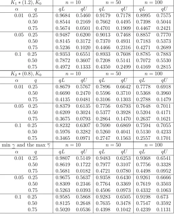
K1K0 n= 10 n= 50 n= 100 α q qL qU qL qU qL qU 0.01 0.25 0.50 0.75 0.9524 0.4640 0.8432 0.0915 0.5807 0.0028 0.8727 0.6028 0.7047 0.2859 0.4629 0.0795 0.8599 0.6357 0.6913 0.3120 0.4400 0.0831 0.05 0.25 0.50 0.75 0.9169 0.5211 0.7686 0.1542 0.5056 0.0112 0.8396 0.6336 0.6447 0.3336 0.4019 0.0995 0.8339 0.6669 0.6450 0.3625 0.3910 0.1193 0.1 0.25 0.50 0.75 0.8941 0.5413 0.7230 0.1878 0.4600 0.0221 0.8193 0.6518 0.6076 0.3521 0.3752 0.1151 0.8218 0.6945 0.6217 0.4096 0.3663 0.1618 K2K0 n= 10 n= 50 n= 100 α q qL qU qL qU qL qU 0.01 0.25 0.50 0.75 0.8828 0.5851 0.7026 0.2563 0.4514 0.0447 0.8196 0.6791 0.6096 0.3971 0.3700 0.1518 0.8118 0.6982 0.6012 0.4088 0.3472 0.1565 0.05 0.25 0.50 0.75 0.8524 0.6135 0.6491 0.3076 0.3939 0.0862 0.7998 0.6960 0.5780 0.4161 0.3338 0.1683 0.7976 0.7135 0.5740 0.4368 0.3186 0.1834 0.1 0.25 0.50 0.75 0.8356 0.6029 0.6169 0.3132 0.3601 0.1266 0.7869 0.7038 0.5587 0.4258 0.3165 0.1781 0.7910 0.7240 0.5622 0.4584 0.3068 0.2042
min γ and the max γ n= 10 n= 50 n= 100
α q qL qU qL qU qL qU 0.01 0.25 0.50 0.75 0.9539 0.4623 0.8468 0.0889 0.5844 0.0027 0.8748 0.5958 0.7081 0.2757 0.4667 0.0656 0.8602 0.6356 0.6915 0.3118 0.4402 0.0826 0.05 0.25 0.50 0.75 0.9216 0.5089 0.7779 0.1484 0.5184 0.0222 0.8450 0.6303 0.6522 0.3267 0.4085 0.0948 0.8357 0.6663 0.6481 0.3614 0.3938 0.1177 0.1 0.25 0.50 0.75 0.9017 0.5064 0.7369 0.1727 0.4782 0.0580 0.8258 0.6476 0.6182 0.3474 0.3824 0.1108 0.8243 0.6896 0.6258 0.4008 0.3714 0.1519
Table 7: Proportion of runs with future observation greater than the quartiles, Arrhenius model,
K1∗(1.2), K0 n= 10 n= 50 n= 100 α q qL qU qL qU qL qU 0.01 0.25 0.50 0.75 0.9684 0.5460 0.8544 0.2169 0.5674 0.0501 0.9179 0.7178 0.7662 0.4495 0.4701 0.1909 0.8995 0.7575 0.7398 0.5044 0.4467 0.2421 0.05 0.25 0.50 0.75 0.9487 0.6200 0.8145 0.3172 0.5236 0.1020 0.9013 0.7468 0.7370 0.4931 0.4466 0.2316 0.8857 0.7770 0.7183 0.5373 0.4271 0.2689 0.1 0.25 0.50 0.75 0.9353 0.6551 0.7872 0.3607 0.4972 0.1333 0.8933 0.7608 0.7208 0.5141 0.4350 0.2499 0.8785 0.7883 0.7072 0.5530 0.4169 0.2815 K2∗(0.8), K0 n= 10 n= 50 n= 100 α q qL qU qL qU qL qU 0.01 0.25 0.50 0.75 0.8679 0.5767 0.6690 0.2470 0.4135 0.0481 0.7896 0.6642 0.5596 0.3710 0.3106 0.1303 0.7778 0.6918 0.5368 0.3960 0.2788 0.1479 0.05 0.25 0.50 0.75 0.8379 0.6135 0.6209 0.3024 0.3675 0.0793 0.7756 0.6793 0.5377 0.3928 0.2864 0.1470 0.7648 0.7011 0.5204 0.4171 0.2637 0.1621 0.1 0.25 0.50 0.75 0.8232 0.6307 0.5976 0.3282 0.3465 0.0971 0.7690 0.6869 0.5260 0.4041 0.2747 0.1563 0.7594 0.7055 0.5130 0.4233 0.2557 0.1701
min γ and the max γ n= 10 n= 50 n= 100
α q qL qU qL qU qL qU 0.01 0.25 0.50 0.75 0.9807 0.5149 0.8619 0.1722 0.5681 0.0182 0.9483 0.6253 0.7977 0.3107 0.4721 0.0780 0.9368 0.6541 0.7756 0.3328 0.4498 0.0952 0.05 0.25 0.50 0.75 0.9675 0.5637 0.8309 0.2346 0.5263 0.0393 0.9358 0.6430 0.7764 0.3369 0.4506 0.0973 0.9261 0.6666 0.7619 0.3503 0.4332 0.1063 0.1 0.25 0.50 0.75 0.9585 0.5868 0.8125 0.2648 0.5020 0.0536 0.9283 0.6505 0.7635 0.3478 0.4398 0.1042 0.9198 0.673 0.7547 0.3592 0.4239 0.1131
Table 8: Proportion of runs with future observation greater than the quartiles, Arrhenius model.
min γ and the max γ n= 10 n= 50 n= 100 γ =γ 1 γ =γ1 γ =γ 1 and γ = γ1 9993 1821 1814 10000 12 12 10000 5 5
Table 9: Number of the simulation runs withγ =γ1 or γ =γ1 or both out of 10,000 simulation
runs with 0.05 level of significance, Arrhenius model.K1∗(1.2) andK2∗(0.8). Case 2.
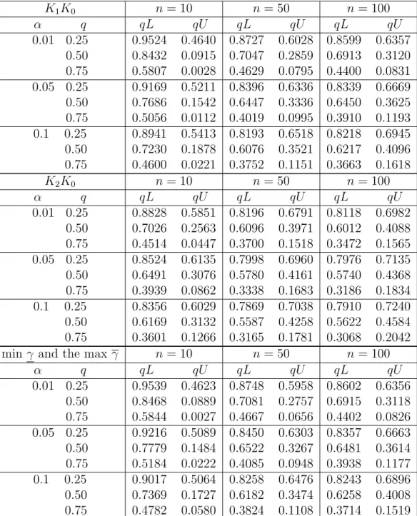
K1K0 n= 10 n= 50 n= 100 α q qL qU qL qU qL qU 0.01 0.25 0.50 0.75 0.9396 0.4970 0.8238 0.1426 0.5694 0.0205 0.8583 0.6306 0.6762 0.3254 0.4338 0.0938 0.8332 0.6718 0.6426 0.3706 0.3889 0.1251 0.05 0.25 0.50 0.75 0.9068 0.5547 0.7573 0.2230 0.5051 0.0477 0.8355 0.6612 0.6350 0.3700 0.3988 0.1264 0.8162 0.6942 0.6089 0.4007 0.3570 0.1544 0.1 0.25 0.50 0.75 0.8887 0.5822 0.7184 0.2630 0.4692 0.0694 0.8244 0.6763 0.6176 0.3908 0.3785 0.1457 0.8084 0.7035 0.5944 0.4165 0.3418 0.1686 K2K0 n= 10 n= 50 n= 100 α q qL qU qL qU qL qU 0.01 0.25 0.50 0.75 0.8782 0.6038 0.6965 0.2848 0.4571 0.0648 0.8072 0.6911 0.5905 0.4053 0.3486 0.1576 0.7959 0.7116 0.5704 0.4336 0.3140 0.1820 0.05 0.25 0.50 0.75 0.8529 0.6407 0.6497 0.3381 0.4047 0.1020 0.7943 0.7054 0.5673 0.4271 0.3265 0.1775 0.7875 0.7204 0.5540 0.4501 0.2970 0.1971 0.1 0.25 0.50 0.75 0.8379 0.6558 0.6261 0.3618 0.3795 0.1222 0.7871 0.7131 0.5571 0.4393 0.3153 0.1883 0.7822 0.7243 0.5455 0.4578 0.2902 0.2056
min γ and the max γ n= 10 n= 50 n= 100
α q qL qU qL qU qL qU 0.01 0.25 0.50 0.75 0.9433 0.4934 0.8281 0.1366 0.5749 0.0153 0.8583 0.6286 0.6777 0.3229 0.4349 0.0916 0.8338 0.6705 0.6435 0.3690 0.3902 0.1238 0.05 0.25 0.50 0.75 0.9133 0.5472 0.7671 0.2116 0.5142 0.0373 0.8376 0.6583 0.6384 0.3650 0.4016 0.1222 0.8176 0.6915 0.6117 0.3975 0.3592 0.1503 0.1 0.25 0.50 0.75 0.8966 0.5723 0.7334 0.2495 0.4800 0.0566 0.8261 0.6727 0.6229 0.3848 0.3831 0.1386 0.8103 0.6999 0.5980 0.4116 0.3445 0.1634
Table 10: Proportion of runs with future observation greater than the quartiles, Eyring model. Case 3.
8. Concluding remarks
This paper has presented statistical methods for ALT using the Arrhenius-Weibull model under constant stress testing, supported by the theory of imprecise probability [3, 4], where the imprecision results from the use of the likelihood
ra-495
tio test [26]. The proposed method applies the use of the likelihood ratio test to compare the survival distribution of pairwise stress levels, in combination with the
Arrhenius model finding the interval of γ values according to the null hypothesis.
The observations at the increased stress levels were transformed to interval-valued observations at the normal stress level by developing imprecision in the link function
500
of the Arrhenius model via a classical test between the pairwise stress levels. We found that using an interval of values for the parameter in the link function between different stress levels enabled us to achieve a greater level of robustness than if we were to use a single point for the parameter. Using the Arrhenius model, we linked the data at different stress levels to the normal stress level, after which NPI can
505
be used at normal stress level. The most pessimistic case, which leads to the lower
survival function S, uses γ to transform the data points to the smallest values at
the normal stress level. Unlike the most optimistic case, which usesγ to transform
the data points to the largest values at the normal stress level.
We discussed the use of pairwise tests instead of one test on all stress levels
510
simultaneously, elsewhere [1]. If the model fits poorly, a single test on all stress levels would result in less imprecision while our proposed method, combining pairwise tests, tends to result in more imprecision. It should be mentioned that we were quite surprised to see that the classical literature in this field mostly presents methods for parameter estimation, with no explicit attention to prediction at the normal
515
stress level. Hence, we did not find classical methods that were suitable for direct
comparison with our method. Using the proposed approach, the intervals [γ, γ]
for the parameter for the link function have adequate imprecision if the model fits well. However, the intervals [γ, γ] for the parameter for the link function get wider if the model fits poorly. The latter can happen if the model assumptions are not
520
fully correct. However, if we have large imprecision, the remaining inferences are probably of no use at all. Therefore, it will be a strong recommendation to do more detailed modelling or to sample more data in such cases. Regarding the choice of the values of the factors for assessing robustness of the methods, we only show that any suggested form of misspecification can be included in simulations to then
525
study the level of robustness. We have shown how the use of different significant levels for the pairwise likelihood ratio tests lead logically to varying imprecision in the final inferences. An interesting topic for future research concerns the choice of the significance level, in particular related to theoretical coverage properties for the final predictive inference resulting from the NPI-based inference in the form of lower
530
and upper survival functions for a future observation at the normal stress level. It should be emphasized here, however, that our aim differs substantially from the usual hypothesis testing in frequentist statistics, as we do not aim at a good test
performance in order to decide between two hypotheses, but we want to provide a method which can also be used if the assumed basic model does not fit well, which
535
will then be indicated by large imprecision.
The application of our novel method in this paper assumed that we have failure
times observed at the normal stress level K0. The assumption of having failure
data at the normal stress level K0 may not be realistic in real world applications. In this case, we can apply our method with basic function to a higher stress level
540
that is above the normal stress level K0. The combined data at that level are then transformed all together to the normal stress levelK0. Investigating this is a topic for future research.
Usually, events of interest in reliability and survival analysis are failure times
[8, 9]. However, such data often includes right-censored observations. The A(n)
545
assumption cannot handle right-censored observations, and demands fully observed data. Coolen and Yan [10] presented a generalization ofA(n), called rc-A(n), which
is suitable for NPI with right-censored data. This method can be used at the
second step in our approach if there are right-censored data, and also the likelihood
ratio test can be applied. So generalizing this method to data including
right-550
censored observations is straightforward. Moreover, a transformation link function, generalizing Equation (3), can also be derived if we allow different shape parameters βifor each leveli, so our method can be generalized in this way as well. Investigating these generalizations, for example to consider the effect of such changes on the imprecision in the resulting lower and upper survival functions is an important topic
555
for future research. Of course, one may want to use a different parametric model at each stress level. As long as the model enables the Arrhenius link function (or a similar link function) to be used to link scale parameters, and transformations of data at higher stress levels to the normal stress levels can be written explicitly as function of a parameter of the link function, then the method as presented in this
560
paper can straightforwardly be adapted. It is also possible to apply the basic idea of our new method without assuming a parametric model at each stress level, but instead using the Arrhenius link function directly to transform observations to the normal stress level. In that case, the likelihood ratio test used in this paper must be replaced by a nonparametric test to determine a range of values for the parameter
565
of the Arrhenius link function for which the transformed data mix well with actual data at the normal stress level. As this approach requires substantially different aspects to be explained compared to the method presented in this paper, it will be presented elsewhere.
As mentioned in the introduction section, there is an increasing literature on more
570
detailed modelling of degradation processes related to accelerated test scenarios. It will be of interest to investigate if the method presented in this paper can also be developed for inference based on such more detailed models. While this will pose substantial challenges, the main idea to avoid very detailed or complicated models through the use of simpler models in combination with imprecision suggests that
575
processes.
Since we began this research, we have not found ALT methods with imprecision in the literature. The classical methods as presented in the literature seem effec-tively to stop at parameter estimates, so no predictions and certainly not predictions
580
explicitly at the normal stress level are considered. Of course, there are more pub-lished imprecise statistical methods for other reliability inferences [8, 9]. The main approach presented in this paper, that is taking a simple model and adding impre-cision to a parameter, then using corresponding transformed data for impreimpre-cision at the level of interest, has not been presented before for any inference problem. One
585
important aspect of ALT applications is the decision of the design of the experi-ment, so which stress levels to use and how many items to use at each level. There is substantial attention to this in the literature on ALT, and we have not addressed it yet in combination with the inferential method presented in this paper, hence this is left as an important topic for future research.
590
As with any novel statistical method developed for real-world applications, the real value of our method should be shown in practical applications. To implement the method, not more is needed on the modelling side then for the classic inference methods with the same model assumptions, but the main questions are how one can use the resulting lower and upper survival functions to support real-world decisions.
595
In continuing research, we are investigating this important aspect in the context of warranty contracts, while it is also interesting to consider the use of our method for other decision support scenarios. Finally, we are starting research into different ALT scenarios, where we aim to develop a similar approach, e.g. for the case of step-stress testing.
600
Acknowledgements
The authors thank two anonymous reviewers for helpful suggestions that have led to improved presentation. Abdullah A.H. Ahmadini gratefully acknowledges the financial support from Jazan University in Saudi Arabia.
References
605
[1] Ahmadini AAH, Coolen FPA (2018, September). Imprecise statistical inference for accelerated life testing data: imprecision related to log-rank test. In Interna-tional Conference Series on Soft Methods in Probability and Statistics, Advances
in Intelligent Systems and Computing (AISC). 823, pp. 1–8. Springer.
[2] Alam K, Sudhir P (2015). Testing equality of scale parameters of two Weibull
dis-610
tributions in the presence of unequal shape parameters.Acta et Commentationes
Universitatis Tartuensis de Mathematica, 19, 11–26.
[3] Augustin T, Coolen FPA (2004). Nonparametric predictive inference and interval probability. Journal of Statistical Planning and Inference, 124, 251–272.
[4] Augustin T, Coolen FPA, de Cooman G, Troffaes MCM (2014).Introduction to
615
Imprecise Probabilities. Wiley, Chichester.
[5] Bretz, F., Genz, A., A. Hothorn, L. (2001). On the numerical availability of
multiple comparison procedures. Biometrical Journal: Journal of Mathematical
Methods in Biosciences, 43, 645-656.
[6] Coolen FPA (2006). On nonparametric predictive inference and objective
620
Bayesianism. Journal of Logic, Language and Information, 15, 21–47.
[7] Coolen FPA (2011). Nonparametric predictive inference.International
Encyclo-pedia of Statistical Science, pp. 968–970. Springer, Berlin.
[8] Coolen FPA, Coolen-Schrijner P, Yan KJ (2002). Nonparametric predictive in-ference in reliability. Reliability Engineering and System Safety, 78, 185–193.
625
[9] Coolen FPA, Utkin LV (2011). Imprecise reliability. In: Lovric, M. (ed.), Inter-national Encyclopedia of Statistical Science, pp. 649–650. Springer, Berlin. [10] Coolen FPA, Yan KJ (2004). Nonparametric predictive inference in reliability.
Reliability Engineering and System Safety, 78, 185–193.
[11] De Finetti B (1974). Theory of Probability. Wiley, Chichester.
630
[12] Duan F, Wang G (2018). Bivariate constant-stress accelerated degradation
model and inference based on the inverse Gaussian process. Journal of
Shang-hai Jiaotong University (Science), 23, 784–790.
[13] Elsayed EA, Zhang H (2007). Design of PH-based accelerated life testing plans
under multiple-stress-type. Reliability Engineering and System Safety, 92, 286–
635
292.
[14] Fan T, Wang W, Balakrishnan N (2008). Exponential progressive step-stress
life-testing with link function based on Box–Cox transformation. Journal of
Sta-tistical Planning and Inference, 138, 2340–2354.
[15] Fard N, Li C (2009). Optimal simple step stress accelerated life test design
640
for reliability prediction. Journal of statistical planning and inference, 139(5), 1799–1802.
[16] Han D (2015). Time and cost constrained optimal designs of constant-stress and step-stress accelerated life tests. Reliability Engineering and System Safety,
140, 1-14.
645
[17] Hill BM (1968). Posterior distribution of percentiles: Bayes’ theorem for
sam-pling from a population. Journal of the American Statistical Association, 63,
[18] Hill BM (1988). De Finetti’s theorem, induction, and Bayesian nonparamet-ric predictive inference (with discussion). Bayesian Statistics 3, (Editors) J.M.
650
Bernando, M.H. DeGroot, D.V. Lindley and A. Smith, pp. 211–241. Oxford Uni-versity Press.
[19] Liao CM, Tseng ST (2006). Optimal design for step-stress accelerated degra-dation tests. IEEE Transactions on Reliability, 55, 59–66.
[20] Meeker WQ, Escobar LA (1998).Statistical Methods for Reliability Data. Wiley,
655
New York.
[21] Meeker WQ, Sarakakis G, Gerokostopoulos A (2013). More pitfalls in conduct-ing and interpretconduct-ing the results of accelerated tests.Journal of Quality Technology,
45, 213–222.
[22] Nasira EA, Pan R (2015). Simulation-based Bayesian optimal ALT designs for
660
model discrimination. Reliability Engineering and System Safety, 134, 1–9.
[23] Nelson WB (1990). Accelerated Testing: Statistical Models, Test Plans, and
Data Analysis. Wiley, Hoboken, New Jersey.
[24] O’Brien, P. C., Fleming, T. R. (1979). A multiple testing procedure for clinical trials. Biometrics, 549-556.
665
[25] Pan Z, Balakrishnan N, Sun Q (2011). Bivariate constant-stress accelerated
degradation model and inference.Communications in Statistics - Simulation and
Computation, 40, 247–257.
[26] Pawitan Y (2001). In all likelihood: Statistical Modelling and Inference using
Likelihood. Oxford University Press.
670
[27] Sha N, Pan R (2014). Bayesian analysis for step-stress accelerated life testing using Weibull proportional hazard model. Statistical Papers,55, 715–726.
[28] Vassilious A, Mettas A (2001). Understanding accelerated life-testing analysis. In Annual Reliability and Maintainability symposium, Tutorial Notes, 1–21. [29] Yin Y, Coolen FPA, Coolen-Maturi TA (2017). An imprecise statistical method
675
for accelerated life testing using the power-Weibull model.Reliability Engineering and System Safety, 167, 158-167.
![Table 2: [γ i , γ i ] for likelihood ratio test](https://thumb-us.123doks.com/thumbv2/123dok_us/613013.2573448/10.918.103.828.748.902/table-γ-γ-likelihood-ratio-test.webp)
![Figure 1: Some transformed data using [4060.018, 6605.752]](https://thumb-us.123doks.com/thumbv2/123dok_us/613013.2573448/11.918.133.727.139.392/figure-some-transformed-data-using.webp)