Approximation schemes for network, clustering and queueing models

(1)

Copyright by

Madhushini Narayana Prasad 2018

(2)

The Dissertation Committee for Madhushini Narayana Prasad certifies that this is the approved version of the following dissertation:

Approximation Schemes for Network, Clustering and

Queueing Models

Committee:

Grani A. Hanasusanto, Supervisor Evdokia Nikolova

Purnamrita Sarkar

(3)

Approximation Schemes for Network, Clustering and

Queueing Models

by

Madhushini Narayana Prasad,

DISSERTATION

Presented to the Faculty of the Graduate School of The University of Texas at Austin

in Partial Fulfillment of the Requirements

for the Degree of

DOCTOR OF PHILOSOPHY

THE UNIVERSITY OF TEXAS AT AUSTIN December 2018

(4)

Dedicated to my husband and son Aran. With blessings of Cheenbol Thatha and Ammamma.

(5)

Acknowledgments

I wish to thank the multitudes of people for making this dissertation pos-sible. First and foremost, I owe my deepest gratitude to my advisor, Dr. Grani Hanasusanto. Without his mentor, support and drive, this entire dissertation would not be possible. I would also like to express my gratitude to Dr. Nedi-alko Dimitrov for his insightful guidance, encouragement and mental support during the first half of my PhD journey. Both of them have been my mentors in numerous ways, showing me not only the charm of research but also the way of being a better person. They are knowledgeable, patient and supportive, and I am really fortunate to have worked with them.

I am grateful to Dr. Evdokia Nikolova for her valuable insights and con-structive feedback throughout this journey, in particular, during my initial work with Dr. Nedialko Dimitrov. Inspite of her busy schedule, she spent a lot of time helping us to define and structure the problem well, and improve the article for journal submission. I would also like to thank my other com-mittee members Dr. Purnamrita Sarkar and Dr. Alexandros Dimakis for being kind and supportive. Discussions with them inspired me to understand and improve my research a lot better.

I am also grateful to Dr. John Hasenbein for offering me several TA posi-tions and for being supportive throughout this journey. I always owe him for his positive feedback to my Queueing course project which led to the final chap-ter of my dissertation. I would also like to thank Dr. Eric Bickel, Dr. Jonathan Bard and Dr. Stephen Boyles for supporting me in various forms during my

(6)

graduate study. I am always indebted to Dr. C. Rajendran of Indian Institute of Technology Madras, for being my (master’s degree) advisor, mentor and well-wisher.

Many thanks to my friends and fellow students in the ORIE. Special thanks to Areesh Mittal and Zachary Smith for always being supportive and ready to help whenever needed. I would also like to thank my other friends, to name a few, Murat Karata˜s, Prateek Srivastava, Bryan Arguello, Joshua Woodruff and Kazunori Nagasawa for making this journey lively and memorable.

Last but not least, my sincere gratitude goes to family, especially my beloved husband and my dear son Aran, for their love and care, and for sharing my frustration and happiness. They are my source of strength on each and every day. Their constant love and encouragement gave me the strength to overcome the challenges I faced during my studies and cheered me up. I thank God for blessing me with more than I could ever hope for, and keeping me protected in his palm.

(7)

Approximation Schemes for Network, Clustering and

Queueing Models

Publication No.

Madhushini Narayana Prasad, Ph.D. The University of Texas at Austin, 2018

Supervisor: Grani A. Hanasusanto

In this dissertation, we consider important optimization problems that arise in three different domains, namely network models, clustering problems and queueing models. To be more specific, we focus on devising efficient traf-fic routing models, deriving exact convex reformulation to the well-knownK -means clustering problem and studying the classical Naor’s observable queues under uncertain parameters. In the following chapters, we discuss these prob-lems in detail, design efficient and tractable solution methodologies, and assess the quality of proposed solutions.

In the first part of the dissertation, we analyze a limited-adaptability traffic routing model for the Austin road network. Routing a person through a traffic network presents a tension between selecting a fixed route that is easy to navi-gate and selecting an aggressively adaptive route that minimizes the expected travel time. We develop non-aggressive adaptive routes in the middle-ground seeking the best of both these extremes. Specifically, these routes still adapt

(8)

to changing traffic condition, however we limit the total number of allowable adjustments. This improves the user experience, by providing a continuum of options between saving travel time and minimizing navigation. We design strategies to model single and multiple route adjustments, and investigate enumerative techniques to solve these models. We also develop tractable al-gorithms with easily computable lower and upper bounds to handle real-size traffic data. We finally present the numerical results highlighting the benefit of different levels of adaptability in terms of reducing the expected travel time. In the second part of the dissertation, we study the well-known classical K-means clustering problem. We show that the popular K-means clustering problem can equivalently be reformulated as a conic program of polynomial size. The arising convex optimization problem is NP-hard, but amenable to a tractable semidefinite programming (SDP) relaxation that is tighter than the current SDP relaxation schemes in the literature. In contrast to the existing schemes, our proposed SDP formulation gives rise to solutions that can be leveraged to identify the clusters. We devise a new approximation algorithm forK-means clustering that utilizes the improved formulation and empirically illustrate its superiority over the state-of-the-art solution schemes.

Finally, we study an extension of Naor’s analysis [74] on the joining or balk-ing problem in observable M/M/1 queues, relaxing the principal assumption of deterministic arrival and service rates. While all the Markovian assumptions still hold, we assume the arrival and service rates are uncertain and study this problem under stochastic and distributionally robust settings. In the former setting, the exact rates are unknown but we assume the distribution of rates are known to all the decision makers. We derive the optimal joining threshold strategies from the perspective of an individual customer, a social optimizer

(9)

and a revenue maximizer, such that expected profit rate is maximized. In the distributionally robust setting, we go a step further to assume the true distributions are unknown and the decision makers have access to only a finite set of training samples. Similar to the stochastic setting, we derive optimal thresholds such that the worst-case expected profit rates are maximized. Fi-nally, we compare our observations, both theoretically and numerically, with Naor’s classical results.

(10)

List of Tables

3.1 Improvement of the true K-means objective value of the clus-ter assignment generated from the Algorithm 1 relative to the ones generated from the algorithm in [72] (left) and the Lloyd’s Algorithm (right). . . 80 4.1 Joining Strategies with Uncertain Arrival and Service Rates . 111

(13)

List of Figures

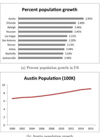
2.1 (a) Top ten US cities ranked based on its percent population growth between 2014 to 2015. (b) Population history of Austin city . . . 7 2.2 Sample routes generated using Google Maps and Waze on Austin

road network. . . 8 2.3 Two state traffic model: Red solid line indicates the possibility

of high traffic on a edge, for example edge (a, b) with probabil-ity 1−pab and travel time dab. Black solid line indicates the possibility of low traffic with probability pab and travel timecab. 12 2.4 An example to show that an adjustment edge need not be a

part of fixed shortest route: Edge weights represent expected travel time. We assume low traffic with probability 1.0 on all the edges except edge (a, t). At edge (a, t) we assumepat as 0.2, cat as 0 and dat as 100 with expected travel time 80. . . 14 2.5 Single Route Adjustment Policy: Solid black line represents an

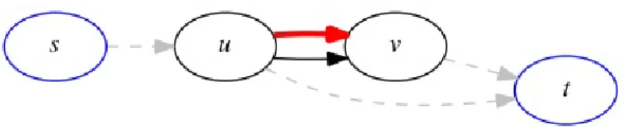
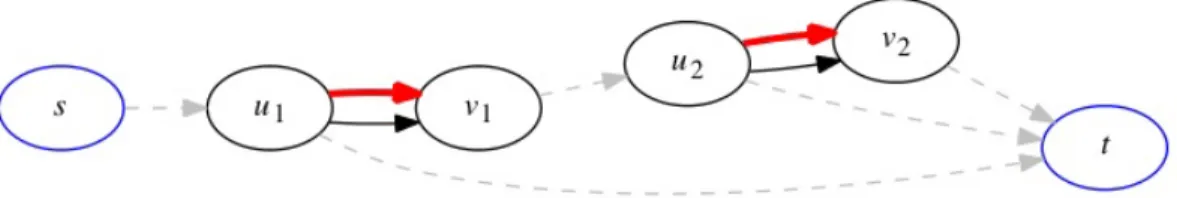
edge. Grey dotted lines represent the shortest paths between the nodes with expected travel time as edge lengths. Solid red line represents the edge to observe for traffic. . . 15 2.6 Series Unforced Model with two adjustment edges . . . 17 2.7 Series Forced Model with two adjustment edges . . . 19 2.8 Example 1 – Expected travel time comparison of series models:

Red solid lines represent the two best adjustment edges for the respective models. . . 21 2.9 Example 2 – Expected travel time comparison of series models:

Red solid lines represent the two best adjustment edges for the respective models. . . 22 2.10 Parallel Model with two adjustment edges . . . 22 2.11 Map of Austin Road Network: Brown colored edges assume p

= 0.4 and d = 5 *c. Red colored edges assume p = 0.5 and d = 4 * c. Remaining edges assume p = 0.6 and d = 3 * c. Blue solid dots represent an example source-destination pair. . . 26 2.12 Pruned network and the set of critical adjustment edges for

the single route adjustment policy: Shaded portion represents the pruned network and the red solid line represents the set of feasible adjustment edges. . . 37

(14)

2.13 Optimal single route adjustment policy: Red solid line sents the optimal adjustment edge. Blue and green lines repre-sent the non-adjusted and the adjusted shortest route respectively. 38 2.14 Optimal two route adjustment policy: Red solid line represents

the optimal adjustment edges. Blue and green lines represent the non-adjusted and the adjusted shortest routes respectively. 39 2.15 Benefit of Adaptability: This graph summarizes the expected

travel time across varying number of adjustment edges. Brown dashed and brown solid lines represent the non-adaptive and completely adaptive expected travel times. Red, green and blue bars represent the summary of series unforced model, series forced and parallel models respectively. . . 41 4.1 Improvement of the Wasserstein policy relative to the SAA

pol-icy in terms of out-of-sample profit rate. The solid blue lines represent the mean, and the error bars visualize the 20% and 80% quantiles of the relative improvement, respectively. . . 112

(15)

Chapter 1

Introduction

1.1

Non-aggressive Adaptive Routing in Traffic

Traffic congestion, resulting from rapid population growth, is a major problem faced by growing cities like Austin. Commuters spend a significant amount of time in traffic and devising an efficient routing strategy to cope with this situation is a major challenge.

Two of the most commonly used products in day-to-day traffic routing are

Google Maps andWaze. These products follow different routing strategies and

serve different purposes. Given a road network with driving times between road intersections, Google Maps yields a static route between a source and destination pair minimizing the total drive time. It is a non-adaptive routing strategy where the route generated does not dynamically change based on the traffic. At the other extreme, Waze produces a completely adaptive route where the path keeps updating with the traffic conditions encountered. This adaptive routing policy results in significantly shorter drive times compared to Google maps, however, the frequent route changes may lead to very high level of navigation stress. In Chapter 2, we aim to develop a middle-ground strategy, which we refer to as anon-aggressive adaptive routing, that combines the advantages of both the policies.

A non-aggressive adaptive route adapts dynamically to changing traffic conditions but in a limited way – for example by allowing only a certain number

(16)

of route-shifts at critical junctures. These routes seek to provide both low travel times and low stress of navigation. We first propose a single route

adjustment policy, where the driver has the potential to observe and adapt at

only one intersection. We compute a best adjustment edge that minimizes the expected travel time, through complete enumeration.

Next, we extend our study to multiple route adjustment policies, where the driver has the potential to make k route adjustments. We consider three different routing strategies what we call,series unforced, series forced and

par-allel models, which differ by how the adjustments are performed on the routes.

We develop dynamic programming based algorithms to compute a best set of k adjustment edges that minimizes the expected travel time. We also propose easily computable lower and upper bounds to improve the tractability of the dynamic programming algorithms and handle large-sized networks. Finally, the performance of our algorithms are evaluated on the Austin road network, in terms of the trade-off between the savings in travel time and increasing lev-els of adaptability. We highlight the contributions of the chapter and suggest some future research directions in Chapter 5.

1.2

Convex Reformulations for K-means Clustering

Consider a set of entities together with observations or measurements de-scribing them. Cluster Analysis deals with the problem of finding subsets of interest called clusters within such a set. Usually, clusters are required to be homogeneous and/or well separated. Homogeneity means that entities within the same cluster should resemble one another. The separation is that enti-ties in different clusters should differ one from the other. This problem is old and can be traced back to Aristotle. It is also ubiquitous, with applications

(17)

in natural sciences, psychology, medicine, engineering, economics, marketing and other fields, and, as a consequence, the literature on cluster analysis is vast. Closely related fields are pattern recognition, computer vision, compu-tational geometry and subfields of operations research such as location theory and scheduling.

A natural measure for homoegeneity/separation is given by the

within-cluster sum of squares. This setting gives rise to the K-means clustering

[70, 68] which is one of the most popular approaches and is widely regarded as the de facto standard for cluster analysis [70, 68, 54]. Given a set of N data points in real D-dimensional space _RD_{, and an integer} _{K, the problem} is to determine a set of K points in _RD, called centroids, to minimize the mean-squared Euclidean distance from each data point to its nearest centroid. A closely related problem to K-means is non-negative matrix factorization with orthogonality constraints (ONMF). The ONMF problem seeks to factor-ize the input data matrix X into two non-negative matrices F and U such that the distance betweenF U> and X is minimized subject to orthogonality constraints.

Given the apparent difficulty of solving theK-means and ONMF problems exactly, it is natural to consider approximations. One of the most popular heuristics for theK-means problem is Lloyd’s algorithm. The algorithm alter-nates between calculating centroids of proto-clusters and reassigning points to the nearest centroid, may in general, converge to local minima. Another recent popular solution scheme is due to convex relaxations [80, 11, 84]. Specifically, Peng and Wei [80] develop a tractable semidefinite programming (SDP) lower bounds for the K-means problem.

(18)

ONMF and the K-means clustering problems through conic programming. We adapt and extend the results by Burer and Dong [28] to reformulate the (non-convex) quadratically constrained quadratic program (QCQP) as a linear program over the convex cone of completely positive matrices. The resulting optimization problem is still NP-hard but replacing the cone of completely positive matrices with its outer-most approximation yields a tractable SDP relaxation to the original problem. We also show that our SDP relaxation is tighter than the well-known relaxation by Peng and Wei [80]. As byproducts of our derivations, we identify a new condition that makes the ONMF and theK-means clustering problems equivalent. We devise a new approximation scheme based on our SDP relaxation, and numerically highlight its superiority, in terms of clustering quality, over the well-known existing approximation schemes. We summarize the contributions of the chapter and suggest potential future research directions in Chapter 5.

1.3

Distributionally Robust Strategic Queues

We consider the balking model for a first-come-first served M/M/1 sys-tem where reneging is not allowed. In Naor’s model for observable queueing systems with known arrival and service rates [74], a newly arriving customer can potentially join the existing queue only if the observed system length is less than a optimal threshold. In other words, he decides to join only if the net benefit from joining is non-negative, otherwise he chooses to balk without any gain or loss. In case of tie, the customer is assumed to join the queue. The sole means to control the non-admission of newly arriving customers be-yond the threshold is by levying tolls. This condition is in striking contrast to the usual assumption (in M/M/1 queue) of serving all the arriving

(19)

cus-tomers, assuming the system is stable (λ < µ). In other words, we implement a strategicM/M/1/n queue wheren denotes the maximum system length we aim to maintain, and thus eliminating the need to assume any steady-state condition. Finally, a reward $R and loss (or cost) $C per unit time in the system is chosen such that any newly arriving customer to an empty server should decide to join, i.e., expected lossC ≤Rµ otherwise the optimal policy is to disband the server and divert the customer stream altogether.

In Chapter 4, we extend the classical Naor’s observable model by relax-ing the principal assumption of a deterministic arrival rateλ and service rate µ. For each scenario, we derive the optimal threshold strategies for

individ-ual or self optimization,social optimization and revenue maximization control

schemes. These schemes differ in the logic by how the net profit rate is con-ceived by the decision makers. While individuals wish to maximize their own expected monetary utility, social optimizers seek to maximize the social benefit rate and revenue maximizers aim to maximize the server’s profit rates.

We study the models in stochastic and distributionally robust settings, and compare our observations with Naor’s classical results. In the stochastic setting, we assume the rates are random and drawn from a known distribution. In contrast, we assume the underlying distribution of the rate parameters is unknown in the distributionally robust setting, and we only have access to N training samples drawn from the true distribution. We derive the optimal threshold strategies that maximize the worst-case expected profit rates, where the worst case is taken over all the distributions in the ambiguity set generated from the training samples. We summarize the contributions of the chapter and suggest probable future research directions in Chapter 5.

(20)

Chapter 2

Non-aggressive Adaptive Routing in Traffic

2.1

Introduction

Some major cities in the US are facing the problem of rapid population growth. Figure 2.1(a) shows the fastest growing cities in the US based on recent census data [91] and the vast majority of US population growth is concentrated in Texas state. The city of Austin in Texas tops the list, as it has over the past five years, with 2.95 percent growth between 2014 and 2015 [17]. Forbes [30] also lists Austin as the fastest growing American city. The population in Austin has increased from 650K in 2000 to 900K in 2015 [33] as shown in Figure 2.1(b) and is expected to increase by at least 30 percent by 2030 [4]. This rapid population growth creates unprecedented problems, major among them being traffic congestion [17]. Already Austin is ranked as the fourth most congested city for the year 2013 by INRIX Inc. [58]. According to their report, due to poor traffic conditions, commuters in Austin spent about 41 hours on average in traffic (three hours more than in 2012) and the the overall travel time increased by 22 percent. Future predicted population growth will worsen the situation. In order to manage the increasing traffic congestion, it is vital to devise efficient routes to avoid traffic in a metro city like Austin.

There are various strategies and tools currently available to develop routes. For example, Google maps and Waze route in different ways and serve a dif-ferent clientele. Google maps creates a fixed static route which is easier to

(21)

(a) Percent population growth in US

(b) Austin population growth

Figure 2.1: (a) Top ten US cities ranked based on its percent population growth between 2014 to 2015. (b) Population history of Austin city

(22)

(a) Google maps: An example (b) Waze: An example

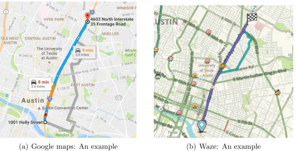
Figure 2.2: Sample routes generated using Google Maps and Waze on Austin road network.

navigate but could be potentially slow. On the other extreme, Waze provides an aggressive adaptive route. A snapshot of routes generated using Google maps and Waze are shown in Figure 2.2(a) and Figure 2.2(b). An (aggres-sive) adaptive route is a potentially faster route that dynamically changes and adapts to traffic conditions but the frequent route changes may lead to high stress in navigation. To alleviate this issue and to create a middle-ground that seeks the best of both extremes, in this chapter, we develop methodology to compute non-aggressive adaptive routes.

A non-aggressive adaptive route adapts dynamically to changing traffic conditions but in a limited way – for example by allowing only a certain num-ber of route-shifts at critical junctures. These routes seek to provide both low travel times and low stress of navigation. At the start of the route, the condi-tions on the roads are only known through a probability distribution. As the driver approaches closer to individual intersections, specific road conditions

(23)

are observed and the routes are adjusted to minimize the travel time.

The main contributions of this chapter are: 1) We propose several strate-gies to model and compute the non-aggressive adaptive routes, based on where and how route adjustments are performed. 2) We develop exact mathematical methods such as complete enumeration and dynamic programming algorithms for each of the strategies. 3) We derive easily computable bounds to solve the models efficiently for large networks. 4) We evaluate and analyze the performance of the models using the Austin road network.

The remainder of the chapter is organized as follows. Section 2 discusses the related work on adaptive routing. Section 3 describes in detail the pro-posed modeling strategies and the respective solution methodologies. Section 4 presents a computational evaluation of the proposed models on the Austin road network. Finally, Section 5 presents our conclusion.

Notation: We denote by _E[(a, b)] the expected travel time on edge (a, b) in the network. The expected travel time of the shortest path from node i to node j is denoted by _E[i → j]. In addition, we denote by _E[i → j|duv] the expected travel time of the shortest path from i to j, given the edge (u, v) is congested. Similarly, _E[i → j|D] denote the expected travel time of the shortest path given that the edges in the setD are congested.

2.2

Related Work

Consider routing a driver from point s to t in a traffic network. Adaptive routing is a stochastic shortest path problem where the edge costs are unknown until arriving at one of its endpoints. The decision to continue or change the

(24)

route is based on the traffic condition at that edge. Croucher [34] appears to be the first to have studied a model of this type but in a fairly restricted setting. In that model, a first-choice arc is selected for every node, there is some probability that arc fails, and if it fails a second outgoing arc is selected at random. Andretta and Romeo [5] considered a similar model with the choice of recourse computed in an optimal way. In their work a recourse path to the destination is computed for every edge, assuming the edge is inactive. In our work, if an edge has traffic congestion, it is still considered active with greater time delay for traversal. However, if an edge is selected for observation and found to be congested, the driver may revert to a recourse route. Unlike the past literature, our work describes a sequence of models in which the driver may observe between one to all edges for traffic congestion.

Another widely studied variant of adaptive routing is the Canadian Trav-eller Problem (CTP). CTP was first defined in [77] (see also ([22])). The goal is to find an optimal routing policy that guarantees a good route under uncertain road conditions, minimizing the expected cost of travel. In this problem, the arc costs are deterministic but unknown and once a road is considered blocked it remains blocked forever. In general, CTP is known to be #P-hard and there has been no significant progress on approximation algorithms. Several variants to this problem such ask−CTP,k−vital edges problem, and deterministic and stochastic recoverable CTP are defined in [16]. Polychronopoulos and Tsit-siklis [82] present another variation to CTP where the realization of arc costs is learned progressively as the graph is traversed. They provide dynamic pro-gramming algorithms to solve models with both dependent and independent arc costs and they establish that the running time of these algorithms is expo-nential in number of arcs. In our work we assume independent arc costs and

(25)

limit the number of re-routing decisions, as opposed to CTP and its variants. We also present tractable dynamic programming algorithms solvable in poly-nomial time. Special cases of CTP are studied by Nikolova and Karger [75] to explore exact solutions. They explain the connection of CTP to Markov Decision Processes (MDPs) solvable in polynomial time. They also present polynomially solvable dynamic programming algorithms for standard version of CTP on directed acyclic graphs (DAGs). It is important to note that our problem is a generic version of CTP. CTP can be derived by equating the number of re-routing decisions to total number of edges in the network, in one of our proposed routing models. Many recent extensions to adaptive routing have been proposed, primarily focusing on route planning under uncertainty for different modes of transportation [25, 24, 73], stability of transportation networks [26], stochastic time dependent networks [45], application to online decision problems [55], and competitive analysis of CTP [95].

To the best of our knowledge, this is the first work on examining non-aggressive adaptive routing, identifying an optimal yet small number of de-cision points on a route. The focus of our work is to derive the benefits of adaptive routing but with limited number of adaptations to reduce driving stress. In lieu of this we propose, compare, and contrast several models for defining the decision points, and develop tractable algorithms to compute the optimal routing policy.

2.3

Model Description

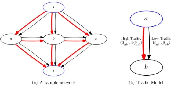
Consider a directed acyclic network G = (N, A), with specified source s and destinationt nodes as shown in Figure 2.3(a). On a city road networkG, N represents the set of road intersections andA represents the set of roads or

(26)

(a) A sample network (b) Traffic Model

Figure 2.3: Two state traffic model: Red solid line indicates the possibility of high traffic on a edge, for example edge (a, b) with probability 1−pab and travel time dab. Black solid line indicates the possibility of low traffic with probabilitypab and travel timecab.

edges connecting those intersections. We consider potential traffic congestion on the edges given by the set A.

We consider a simple model of traffic congestion where each edge is in either a high traffic state or low traffic state, independently of other edges. The traffic probability distribution is assumed to be known ahead of time. Every edge e= (a, b) is defined by three inputs: e= (c, d, p) wherecab represents the travel time under low traffic,dab represents the travel time due to high traffic, and pab represents the probability of low traffic on the edge. This is visually depicted in Figure 2.3(b).

Given these inputs, we determine the edges to be observed for traffic con-gestion and the corresponding adjustment routes should high traffic states be observed on those edges. We call an edge selected for observation and for pos-sible route adjustment asadjustment edge. When the driver reaches the source

(27)

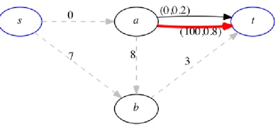
node of an adjustment edge and observes low traffic, they proceed through the edge. If the driver observes high traffic, then they take an adjustment route. To simplify the exposition, we start with a single route adjustment and then provide several extensions to multiple route adjustments. A detailed discussion on these route adjustment strategies is presented in the following subsections. We begin with a simple example presented in Figure 2.4. This example shows that the optimal adjustment edge need not be a part of the fixed non-adaptive shortest route. The shortest path from s to t can be computed as s →b→twith expected travel time 10. If edge (a, t) is observed, there is 20% chance of low traffic with zero travel time. However, there is 80% chance of high traffic at edge (a, t), and if the driver adjusts the route to a→b→tthen the travel time is 11. With the single observation of edge (a, t), the expected travel time is 11·0.8 + 0·0.2 = 8.8, which is lower than the expected travel time without any adjustments (=10). An interesting aspect of this example is that the edge (a, t) is not on the no-adjustment shortest path.

2.3.1 Single Route Adjustment Policy

A pictorial representation of a single route adjustment policy is shown in Figure 2.5, where the route from source s to destination t has a single adjustment edge, (u, v). In this policy, the driver takes the shortest path from s to u, and observes edge (u, v) for traffic. In case of low traffic, the driver continues on the edge (u, v) and takes the shortest path from v to t. In case of high traffic, the driver takes an adjustment route from u to t. The overall expected travel time for any adjustment edge (u, v) is computed using

(28)

Figure 2.4: An example to show that an adjustment edge need not be a part of fixed shortest route: Edge weights represent expected travel time. We assume low traffic with probability 1.0 on all the edges except edge (a, t). At edge (a, t) we assume pat as 0.2, cat as 0 and dat as 100 with expected travel time 80.

where_E[i→j] represents the expected travel time of a no-adjustment shortest path from node i to j, _E[i → j|dik] represents the expected travel time of a no-adjustment shortest path given edge (i, k) is congested, and _E1[(u, v)] rep-resents the expected travel time of a single route adjustment policy using the adjustment edge (u, v). One could determine the adjustment edge that yields minimal expected travel time, arg min(u,v)E1[(u, v)], using complete enumera-tion given by Z1[s →t] =min E[s→t]; min (u,v)∈AE1[(u, v)] , (2.2) where Z1[s →t] represents the overall minimum expected travel time from s totdue to single route adjustment policy. An equivalent integer programming formulation is presented in Appendix A.1.

(29)

Figure 2.5: Single Route Adjustment Policy: Solid black line represents an edge. Grey dotted lines represent the shortest paths between the nodes with expected travel time as edge lengths. Solid red line represents the edge to observe for traffic.

2.3.2 Multiple Route Adjustment Policy

There are several potential models for multiple route adjustments. We present and explore three different strategies that we call the series unforced,

series forced and parallel models. We develop dynamic-programming-based

algorithms to solve these route adjustment models, and finally compare their performances.

Series Unforced Model

Let us start with two adjustment edges as shown in Figure 2.6, which follow what we call a series unforced model. In this model, once the driver makes a route adjustment he loses the potential to observe the other edges for traffic. Say for instance the sourcesand destinationt nodes are connected by a highway. The driver enters the highway from source s, and upon arriving at u1 observes edge (u1, v1) for traffic. In case of high traffic, driver adjusts the route to reach the destination t and never gets to make any other route adjustments. In case of low traffic, driver traverses the edge (u1, v1), continues on the highway untilu2 where they observe edge (u2, v2) for traffic. In case of high traffic at (u2, v2), driver adjusts the route to destinationt. In case of low traffic, driver traverses the edge (u2, v2), continues on the highway to reach

(30)

the destination t.

Let _Esuf[(u1, v1),(u2, v2)] denote the expected travel time with respect to the adjustment edges (u1, v1) and (u2, v2). One could find a pair of edges that yield a minimum expected travel time, arg min(u1,v1)(u2,v2)Esuf[(u1, v1),(u2, v2)], through complete enumeration using

Esuf[(u1, v1),(u2, v2)] =

E[s→u1]+(1−pu1v1)E[u1 →t|du1v1] +pu1v1

cu1v1 +E[v1 →u2] +pu2v2[cu2v2 +E[v2 →t]] + (1−pu2v2)E[u2 →t|du2v2]

. (2.3) The first summand is the expected travel time from s to u1. The second summand is the expected travel time from u1 to t if high traffic is observed at (u1, v1). The third summand is the travel time from u1 to t if low traffic is observed at (u1, v1). This third summand includes within it a version of (2.1), computing the travel time from v1 to t dependent on the observation of traffic at edge (u2, v2). Similarly, one could express the computation of the minimum expected travel time with k adjustment edges recursively with the equation for k−1 adjustment edges as follows. Let Z_ksuf[s → t] denote the overall minimum expected travel time whenk adjustment edges are observed

(31)

Figure 2.6: Series Unforced Model with two adjustment edges for traffic. We can then write

Z₁suf[s →t] =Z1[s →t],and Z_ksuf[s →t] = min Z_ksuf₋₁[s→t]; min (u,v)∈A E[s→u] + (1−puv)E[u→t|duv] +puv(cuv+Zksuf−1[v →t]) . (2.4)

The basecase Zsuf

1 [s → t] represents the minimum expected travel time for a single adjustment edge. The recursive equation to compute Zsuf

k [s → t] includes a Z_ksuf₋₁[s → t] in case it is unnecessary to observe k edges. The second term involves picking the first edge (u, v) for observation, and the remaining length of the paths to destination is based on the probabilities of that observation.

The recursive equation yields a dynamic programming algorithm for com-puting the best set of adjustment edges. The dynamic programming algorithm reduces the computational effort from O(mk), roughly what is required with complete enumeration, toO(mk) wherem =|A|. This brings significant com-putational savings, though as we’ll discuss later, still insufficient for practical applications.

(32)

Series Forced Model

An alternate model with two adjustment edges, which we callseries forced, is depicted in Figure 2.7. In this model, the driver is forced to observe all the adjustment edges, hence has the potential to adjust the route at every such adjustment edge. Consider the same instance where the driver enters the highway from source s and observes an edge (u1, v1) for traffic. In case of high traffic, driver adjusts the route but returns to the next source node u2 to observe adjustment edge (u2, v2). In case of low traffic, driver traverses the edge (u1, v1), continues on the highway until u2 where they observe edge (u2, v2) for traffic. In case of high traffic at (u2, v2), driver adjusts the route to destinationt. In case of low traffic, driver traverses the edge (u2, v2), continues on the highway to reach the destinationt. In this model, driver always observes all the adjustment edges irrespective of the traffic states of previous adjustment edges.

Let _Esf[(u1, v1),(u2, v2)] denote the expected travel time if adjustment edges (u1, v1) and (u2, v2) are selected. One could find a pair of adjust-ment edges that yield a minimum expected travel time, which is given by arg min(u1,v1)(u2,v2)Esf[(u1, v1),(u2, v2)], through complete enumeration using

Esf[(u1, v1),(u2, v2)] =

E[s→u1] +pu1v1[cu1v1 +E[v1 →u2]] + (1−pu1v1)E[u1 →u2|du1v1]

+

pu2v2[cu2v2+E[v2 →t]] + (1−pu2v2)E[u2 →t|du2v2]

. (2.5)

(33)

Figure 2.7: Series Forced Model with two adjustment edges

The first summand is the expected travel time from s to u2. This first summand includes within it a version of (2.1), computing the travel time from s to u2 dependent on the observation of edge (u1, v1). The second summand is the expected travel time fromu2 tot with traffic state observed at (u2, v2). Thus (2.5) can be expressed as a recursive equation as follows,

Z₁sf[s →t] =Z1[s →t],and Z_ksf[s →t] = min Z_ksf₋₁[s→t]; min (u,v)∈A Z_ksf₋₁[s →u] +puv(cuv+E[v →t]) + (1−puv)E[u→t|duv] , (2.6) where Zsf

k[s → t] denotes the overall minimum expected travel time obtained using the series forced model when k adjustment edges are observed for traf-fic. Though inefficient, an integer programming formulation for this model is presented in Appendix A.2.

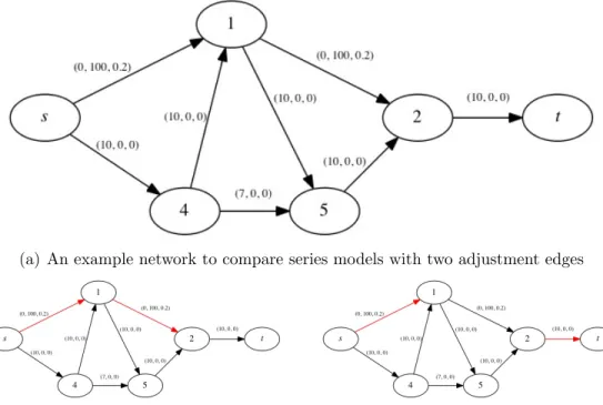
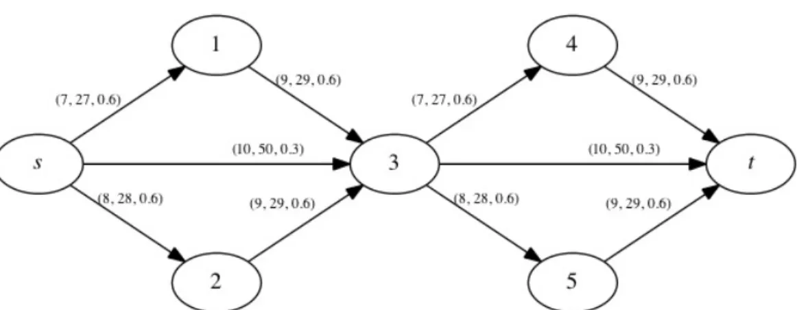
Neither the series unforced nor the forced models are always better in terms of reducing expected travel time. Let us consider the example network in Figure 2.8(a). The edge weights (c, d, p) represent the travel time under low traffic, the travel time under high traffic and the probability of low traffic respectively. The expected travel time of the series models are computed using (2.4) and (2.6), and the resulting best adjustment edges are highlighted

(34)

in Figure 2.8(b) and Figure 2.8(c) respectively. We obtain Zsuf

2 [s→t] as 34.8 andZ₂sf[s→t] as 35.6, with series unforced model performing better than the series forced model. Let us now consider another example network as in Figure 2.9(a). We follow the same routine to obtainZsuf

2 [s→t] as 55.4 andZ2sf[s→t] as 50.8. In this network, series forced model performs better than the series unforced model. This shows that the performance of the series models are incomparable, and it depends on the network instance considered. Generally one may think that the series forced model should perform better, because it has the ability to execute several observations in sequence as opposed to just one. However, as these examples demonstrate, it may be too expensive to execute the secondary observations, as compared to the series unforced model.

Parallel Model

Another model with two adjustment edges, which we call parallel, is de-picted in Figure 2.10. In this model, the driver has the potential to observe edges and make route adjustments, in both the original and adjustment routes. Consider the same instance where the driver enters the highway from source s and observes an edge (u11, v11) for traffic. In case of low traffic, driver traverses the edge (u11, v11), continues on the highway until u12 where they observe edge (u12, v12) for traffic. In case of high traffic at (u11, v11), driver adjusts the route to reach node u22 and observes an edge (u22, v22) for traffic in the adjusted route. In case of high traffic at the second adjustment edge ((u12, v12) or (u22, v22)), driver adjusts the route to destinationt. In case of low traffic, driver traverses the edge, continues on the route to reach the destina-tion t. Unlike series models, driver observes different adjustment edges based on the traffic state of the previous adjustment edges.

(35)

(a) An example network to compare series models with two adjustment edges

(b) Solution: Series Unforced Model (c) Solution: Series Forced Model

Figure 2.8: Example 1 – Expected travel time comparison of series models: Red solid lines represent the two best adjustment edges for the respective models.

(36)

(a) Another example network to compare series models with two adjustment edges

(b) Solution: Series Unforced and Forced Models

Figure 2.9: Example 2 – Expected travel time comparison of series models: Red solid lines represent the two best adjustment edges for the respective models.

(37)

Let _Epll[(u11, v11),(u12, v12),(u22, v22)] denote the expected travel time if adjustment edges (u11, v11), (u12, v12), and (u22, v22) are selected. One could find a set of adjustment edges that yield a minimum expected travel time, arg min(u11,v11),(u12,v12),(u22,v22)Epll[(u11, v11),(u12, v12),(u22, v22)], through com-plete enumeration using

Epll[(u11, v11),(u12, v12),(u22, v22)] = E[s→u11] +pu11v11[cu11v11+ E[v11→u12] +pu12v12[cu12v12 +E[v12→t]] + (1−pu12v12)E[u12→t|du12v12] ] + (1−pu11v11)

E[u11→u22|du11v11] +pu22v22[cu22v22+E[v22 →t]] + (1−pu22v22)E[u22 →t|du22v22]

(2.7) The first summand is the expected travel time from s tou11. The second and third summands together represent the weighted sum of expected travel times fromu11tot, with weights representing the traffic state at (u11, v11). The second summand includes within it a version of (2.1), computing the travel time from v11 tot dependent on the observation of edge (u12, v12). The third summand includes within it a modified version of (2.1). The difference being in the first term where we compute the expected travel time from u11 to u22 given high traffic is observed at (u11, v11).

Let Z_kpll[s → t] denote the overall minimum expected travel time from s to t with k adjustment edges. It is to be noted that the driver’s policy may include more than k adjustment edges, but only k edges will be observed in

(38)

total as they travel from s to t. We now express (2.7) as recursive equations as follows, Z₁pll[s →t] =Z1[s →t], Z_kpll[s →t] = min Z_kpll₋₁[s→t]; min (u,v)∈A E[s →u] +puv(cuv+Z_kpll−1[v →t]) + (1−puv)Zkpll−1[u→t|{duv}] ,and Z₁pll[g →i|D] = min min (g,v)∈A−D pgv(cgv+E[v →i]) + (1−pgv)E[g →i|D∪ {dgv}] , min (u6=g,v)∈A E[g →u|D] +puv(cuv+E[v →i]) + (1−puv)E[u→i|{duv}] , Z_kpll[g →i|D] = min min (g,v)∈A−D pgv(cgv+Z_kpll−1[v →i]) + (1−pgv)Zkpll−1[g →i|D∪ {dgv}] , min (u6=g,v)∈A E[g →u|D] +puv(cuv+Zkpll−1[v →i]) (2.8) + (1−puv)Z_kpll₋₁[u→i|{duv}] ,

whereZ_kpll[g →i|D] denotes the minimum expected travel time from anygtoi given that high traffic is observed at all edges in setD={dg,j1, dg,j2, . . . , dg,jk−1}.

It is easy to see that the series models are the special cases of parallel model, i.e., a solution to a series model can be expressed as a solution to the corresponding parallel model. Hence, the parallel model always outper-forms the series models in terms of reducing travel time, but at the expense of

(39)

more computational effort. It also follows that a parallel model reduces to a Canadian Traveller Problem (CTP) on directed acyclic graphs (DAGs) when all the edges in the network are observed for traffic, i.e., k equals |A|. Thus the proposed dynamic programming algorithm can be used to solve CTP on DAGs. The dynamic programming algorithm proposed in [75] differs from our algorithm mainly by the following two points: 1) In [75], an optimal outgoing edge is computed upon arrival at a node as the graph is traversed. This is dif-ferent from our dynamic programming approach where we pre-compute both the original and the adjustment routes to the destination. 2) The algorithm [75] iterates over all the edges in the network whereas our algorithm is made to stop when observing more adjustment edges no longer reduces the expected travel time.

2.4

Large Scale Tractable Algorithms

We use the Austin road network (Figure 2.11) to evaluate the performance of our proposed models. The travel times c on the edges are known1_{, and} we assume the probability of low traffic and delay offsets based on the street type. The network consists of about 100,000 edges and it is impractical to find the best adjustment edges, even in a single route adjustment policy, through complete enumeration. For example, it takes about 6 hours to find a single adjustment edge for the example source-destination pair shown in Figure 2.11. Inspired by the traditional branch and bound techniques, we develop easily computable lower and upper bounds to eliminate many possibilities and create truly tractable algorithms.

(40)

Figure 2.11: Map of Austin Road Network: Brown colored edges assumep = 0.4 andd= 5 *c. Red colored edges assumep= 0.5 andd= 4 *c. Remaining edges assume p = 0.6 and d = 3 * c. Blue solid dots represent an example source-destination pair.

(41)

2.4.1 Network Pruning

We first focus on developing some easily computable upper and lower bounds to prune the network size. This improves the run time of the shortest path procedures and consequently, the tractability of the proposed dynamic programming algorithms.

LetZ_kM[s→t] represent the minimum expected travel time withk adjust-ment edges and any route adjustadjust-ment model M.

Lemma 2.4.1. The minimum expected travel time between two nodes s and

t are non-decreasing with k adjustment edges, i.e., _E[s → t] ≥ Z1[s → t] ≥

ZM

2 [s→t]≥ · · · ≥ZkM−1[s→t]≥ZkM[s→t].

Proof. The recursive equation (2.8) shows that Z_kpll[s → t] ≤ Z_kpll₋₁[s → t], for any k ≥ 2. Recursively we can write, Z1[s → t] ≥ Z2pll[s → t] ≥ · · · ≥ Z_kpll₋₁[s → t] ≥ Z_kpll[s → t]. To show _E[s → t] ≥ Z1[s → t], consider an edge (u, v) on the shortest path from s tot. Then the expected travel time of shortest path,_E[s→t] can be written as

E[s →t] =E[s→u] +puvcuv+ (1−puv)duv+E[v →t]. (2.9) A term-by-term comparison of (2.9) with (2.1) shows that _E[s → t] is an upper bound to _E1[(u, v)] because going through a high traffic edge (u, v) is one potential routing for_E[u→t|duv]. Thus, _E[s→t] is an upper bound to Z1[s → t]. Using similar logic, the lemma can be proved for the series forced and unforced models as well.

Let us assume there exists an optimal policyπ that includes edge (i, j) on one of the paths generated and letZk(π) be the corresponding expected travel

(42)

time. A lower bound on the travel time of any path going through edge (i, j) can be given by,

LBP(i, j) = cs→i+cij +cj→t. (2.10) where ci→j represents the shortest path from i to j with edge lengths c, i.e., assuming low traffic on all the edges.

Letρ= min

(u,v)∈A{puv,1−puv}. In other words, the probabilities of low traffic are bounded away from (0, 1) by at leastρ. Under a single route adjustment, every path occurs in policy π with probability at least ρ. Under k route adjustments, every path occurs with probability at leastρk_{. This leads to the} following lemma defining a lower bound on any policy that uses edge (i, j).

Lemma 2.4.2. Every k-route adjustment policy π that includes edge (i, j) on some path has Zk(π)≥ρkLBP(i, j) + (1−ρk)cs→t.

Proof. Any path with edge (i, j) occurs with probability at least ρk and has

length at leastLBP(i, j). All other paths in the policy π have length at least cs→t.

Now, we are ready to present our theorem on network pruning.

Theorem 2.4.3. An edge (i0, j0) withρk_LBP_(i0_{, j}0_{) + (1}₋_ρk_)c

s→t>E[s→t],

for any k ≥1, will not be on any path in the optimal routing policy.

Proof. Let π denote the optimal routing policy. By Lemma 2.4.2, we have

Zk(π)≥ ρkLBP(i0, j0) + (1−ρk)cs→t. If Zk(π) >E[s → t], by Lemma 2.4.1, π is not an optimal routing policy. Hence the edge (i0, j0) will not be on any path of the optimal policy π.

(43)

Using the result of Theorem 2.4.3, one can prune the network eliminating several possibilities. For the example source-destination pair considered, and fork = 1 andρ= 0.4, the network is pruned to 17,328 edges.

2.4.2 Critical Adjustment Edges

In addition to pruning the network size, it is also possible to obtain a set of critical adjustment edges that contain the optimal solution. To do this, we employ different lower bounds as discussed in this section.

Lemma 2.4.4. An optimal single route adjustment policy π with adjustment edge (u, v) has Z1(π)≥LBA1(u, v), where LBA1(u, v) is given by

LBA1(u, v) =E[s→u] +cuv+E[v →t].

Proof. By definition, we have duv > cuv. Edge (u, v) is an optimal adjustment

edge, so using (2.1) and (2.2) we get, Z1(π) = min

(u0_,v0₎_∈_AE1[(u

0

, v0)]

=_E[s →u] +puv(cuv+E[v →t]) + (1−puv)E[u→t|duv]. We proceed to complete the proof by contradiction.

Assume _E[u → t | duv] < cuv+E[v →t]. Consider a policy π0 that uses no adjustment edge and the route_E[s→u] is followed by_E[u→t|duv]. Thus the policy π0 has length _E[s → u] +_E[u → t|duv] < E[s → u] +puv(cuv +

E[v → t]) + (1 −puv)E[u → t|duv], implying π is not optimal. This yields

(44)

Using this result, we have

Z1(π) =E[s→u] +puv(cuv+E[v →t]) + (1−puv)E[u→t|duv]

≥_E[s→u] +puv(cuv+E[v →t]) + (1−puv)(cuv+E[v →t])

≥_E[s→u] + (cuv+E[v →t]).

We define the following variables to simplify our notations in the remainder of the section. One can easily pre-compute these quantities and use as required in the upcoming lower bounds for multiple route adjustment policies.

∫[j] = max (a,b)∈A(1−pab) dab+E[b →j]−E[a→j|dab] , §[j] = max (a,b)∈A(1−pab) E[a→j|dab] , α= max

(a,b)∈Apab and β = maxj∈N ∫[j]. (2.11)

Lemma 2.4.5. (Series unforced model) An optimal route adjustment policy π

with edge(u, v) as its first adjustment edge hasZ_ksuf(π)≥LBAsuf_k (u, v), where

LBAsuf

k (u, v) is given by

LBAsuf_k (u, v) =_E[s→u] +cuv+E[v →t]− ∫[t]

k−2

X

k0₌₀

αk0. (2.12)

Proof. Because π is an optimal policy and edge (u, v) is the first adjustment

edge, using (2.4) we have

Z_ksuf(π) = _E[s →u] + (1−puv)E[u→t|duv] +puv(cuv+Zksuf−1[v →t]). We show _E[u → t|duv] ≥ cuv +Zksuf−1[v → t], by contradiction. Assume

E[u→t|duv]< cuv+Zksuf−1[v →t]. Consider a policyπ

(45)

edges and the route _E[s → u] is followed by _E[u → t|duv]. Thus the policy π0 has length_E[s → u] +_E[u →t|duv] <_E[s → u] + (1−puv)_E[u → t|duv] + puv(cuv +Zksuf−1[v → t]), implying π is not optimal. Thus E[u → t|duv] ≥ cuv+Zksuf−1[v →t].

Using this result we have,

Z_ksuf(π) = _E[s→u] + (1−puv)_E[u→t|duv] +puv(cuv+Z_ksuf−1[v →t])

≥_E[s→u] + (1−puv)(cuv+Zksuf−1[v →t]) +puv(cuv+Zksuf−1[v →t])

≥_E[s→u] +cuv+Zksuf−1[v →t]. (2.13) This is a valid yet intractable lower bound to Z_ksuf(π). To alleviate this issue, we derive a lower bound for Zsuf

k−1[v →t]. The potential saving in travel time fromi toj due to single route adjustment policy (using (2.1) and (2.4)), is given by E[i→j]−Z1[i→j]≤E[i→j]− min (u,v)∈A(E[i→u] +puv(cuv+E[v →j]) + (1−puv)E[u→j|duv]) ≤ max (u,v)∈A E[i→u] +puv(cuv+E[v →j]) + (1−puv)(duv+E[v →j]) −(_E[i→u] +puv(cuv+E[v →j]) + (1−puv)E[u→j|duv]) ≤ max (u,v)∈A(1−puv) duv+_E[v →j]−_E[u→j|duv] =∫[j]. (2.14)

It is important to note that (2.14) holds for all route adjustment models since Zsuf

1 [i→j] =Z1sf[i→j] =Z pll

(46)

The potential savings in travel time fromitojdue to two route adjustment policy is given by,

Z1[i→j]−Z2suf[i→j]≤ max (u,v)∈A E[i→u] +puv(cuv+E[v →j]) + (1−puv)E[u→j|duv] −(_E[i→u] +puv(cuv+Z1[v →j]) + (1−puv)E[u→j|duv]) ≤ max (u,v)∈A puv(E[v →j]−Z1[v →j]) ≤ max (u,v)∈Apuv∫[j] =α.∫[j].

The penultimate inequality is due to (2.14). Combining this result with (2.13) fork = 3, we get

Z₃suf(π)≥_E[s→u] +cuv+Z₂suf[v →t]

≥_E[s→u] +cuv+Z1[v →t]−α∫[t]

≥_E[s→u] +cuv+E[v →t]− ∫[t]−α∫[t]. Extending this logic to any k yields,

Z_ksuf(π)≥_E[s→u] +cuv+E[v →t])− ∫[t] k−2

X

k0₌₀

αk0.

Lemma 2.4.6. (Series forced model) An optimal route adjustment policy π

with edge (u, v) as its last adjustment edge has Z_ksf(π) ≥ LBAsf_k(u, v), where

LBAsf

k(u, v) is given by

(47)

Proof. Because π is an optimal policy and edge (u, v) is the last adjustment edge, using (2.6) we have

Z_ksf(π) =Z_ksf₋₁[s→u] +puv(cuv+E[v →t]) + (1−puv)E[u→t|duv]. Given edge (u, v) is the optimal adjustment edge, we show_E[u→t|duv]≥

cuv+E[v →t] following the same procedure as in the proof of Lemma 2.4.5. Assume _E[u→t|duv]< cuv+E[v →t]. Consider a policy π0 that uses only

the first k−1 adjustment edges of π in the same sequence and does not use the last adjustment edge. In other words, the route Zsf

k−1[s → u] is followed by_E[u→t|duv]. Thus the policy π0 has length Zksf−1[s →u] +E[u→ t|duv]< Zsf

k−1[s → u] + (1−puv)E[u → t|duv] +puv(cuv +E[v → t]), implying π is not optimal. Thus _E[u → t|duv] ≥ cuv +E[v → t], given (u, v) is the last adjustment edge.

Z_ksf(π) =Z_ksf₋₁[s→u] +puv(cuv+E[v →t]) + (1−puv)E[u→t|duv]

≥Z_ksf₋₁[s →u] +puv(cuv+E[v →t]) + (1−puv)(cuv+E[v →t])

≥Z_ksf₋₁[s →u] +cuv+E[v →t]. (2.15) We now proceed to obtain a tractable lower bound on Z_ksf₋₁[s →u]. The potential saving in travel time fromi toj due to two route adjustment policy using (2.6), is given by Z1[i→j]−Z2sf[i→j]≤ max (u,v)∈A Z1[i→j]−(Z1[i→u] +puv(cuv+E[v →j]) + (1−puv)E[u→j|duv]) ≤ max (u,v)∈A(E[i→u]−Z1[i→u]) ≤ max (u,v)∈A∫[j] =β.

(48)

The penultimate inequality is due to (2.14). Combining this result with (2.15) fork = 3 yields,

Z₃sf(π)≥Z₂sf[s→u] +cuv+E[v →t]

≥Z1[s→u]−β+cuv+E[v →t]

≥_E[s→u]− ∫[u]−β+cuv+E[v →t].

By extending the logic to a generic k, we obtain

Z_ksf(π)≥_E[s→u]− ∫[u]−(k−2)β+cuv+E[v →t].

Lemma 2.4.7. (Parallel model) An optimal route adjustment policy π with edge (u, v) as its first adjustment edge has Z_kpll(π) ≥ LBApll_k (u, v), where

LBApll_k (u, v) is given by

LBApll_k (u, v) =_E[s→u] +cuv+E[v →t]− ∫[t]

k−2

X

k0₌₀

αk0−(k−2)§[t].

Proof. Because π is an optimal policy and edge (u, v) is the first adjustment

edge, using (2.8) we have

Z_kpll(π) =_E[s→u] + (1−puv)Z_kpll−1[u→t|{duv}] +puv(cuv+Z pll

k−1[v →t]). We showZ_kpll₋₁[u→t|{duv}]≥cuv+Z_kpll₋₁[v →t], by contradiction. Assume Z_kpll₋₁[u → t|{duv}] < cuv+Zkpll−1[v → t]. Consider a policy π

0 _{that uses the}

k−1 adjustment edges of the first adjusted route ofπ (in the same sequence) and does not use any other adjustment edges. In other words, route_E[s →u] is followed by Z_kpll₋₁[u → t|{duv}]. Thus the policy π0 has length E[s → u] +

(49)

Z_kpll₋₁[u → t|{duv}] < E[s → u] + (1−puv)Zkpll−1[u → t|{duv}] + puv(cuv + Z_kpll₋₁[v → t]), implying π is not optimal. Thus Z_kpll₋₁[u → t|{duv}] ≥ cuv + Z_kpll₋₁[v →t].

Z_kpll(π) = _E[s →u] + (1−puv)Zkpll−1[u→t|{duv}] +puv(cuv+Zkpll−1[v →t])

≥_E[s→u] + (1−puv)(cuv+Zkpll−1[v →t]) +puv(cuv+Zkpll−1[v →t])

≥_E[s→u] +cuv+Zkpll−1[v →t]. (2.16) We follow the same procedure as in proof of Lemma 2.4.5 and 2.4.6 to obtain a lower bound onZ_kpll₋₁[v →t]. The potential saving in travel time from ito j due to two route adjustment policy using (2.8),is given by

Z1[i→j]−Z2pll[i→j]≤ max (u,v)∈A Z1[i→j]−(E[i→u] +puv(cuv+Z1[v →j]) + (1−puv)Z1[u→j|duv]) ≤ max (u,v)∈A puv(E[v →j]−Z1[v →j]) + (1−puv)(E[u→j|duv]−Z1[u→j|duv]) ≤ max (u,v)∈A puv∫[j] + max (u,v)∈A (1−puv)E[u→j|duv] =α∫[j] +§[j].

The penultimate inequality is due to the fact that Z1[u→j|duv]≥0 and due to (2.14).

(50)

adjustment policy is given by, Z₂pll[i→j]−Z₃pll[i→j]≤ max (u,v)∈A puv(Z1[v →j]−Z pll 2 [v →j]) + (1−puv)(Z1[u→j|duv]−Z2pll[u→j|duv]) ≤ max (u,v)∈A puv(α∫[j] +§[j]) + (1−puv)E[u→j|duv] ≤α2∫[j] +§[j].

The penultimate inequality is due to the fact that Z₂pll[u → j|duv] ≥ 0 and Z1[u →j|duv]≤E[u→j|duv]. Using the above results in (2.16) for k = 4, we get Z₄pll(π)≥_E[s→u] +cuv+Z3pll[v →t] ≥_E[s→u] +cuv+Z2pll[v →t]−α 2_∫_[t]_{− §}_[t] ≥_E[s→u] +cuv+Z1pll[v →t]−α∫[t]− §[t]−α 2_∫_[t]_{− §}_[t] ≥_E[s→u] +cuv+E[v →t]− ∫[t](1 +α+α2)−2§[t]. By similar logic we derive for any k,

Z_kpll(π)≥_E[s→u] +cuv+E[v →t])− ∫[t] k−2

X

k0₌₀

αk0 −(k−2)§[t].

SinceZ_kpll(π|D)≥Z_kpll(π) by definition,LBApll_k (u, v) is a valid lower bound toZ_kpll(π|D).

Now, we present our theorem to obatin a set of feasible adjustment edges.

Theorem 2.4.8. For any k≥1, an edge(u0, v0)withLBA1(u0, v0)>E[s→t]

or LBAM

k(u

0_{, v}0₎ _{> Z}M

k−1[s → t], cannot be the first adjustment edge (for M

being series unforced or parallel model) or the last adjustment edge (for M being series forced model) in an optimal routing policy.

(51)

Figure 2.12: Pruned network and the set of critical adjustment edges for the single route adjustment policy: Shaded portion represents the pruned network and the red solid line represents the set of feasible adjustment edges.

Proof. Let π be a routing policy using series unforced model and edge (u0, v0)

as the first adjustment edge.

We show that π is not optimal if LBAsuf k (u

0_{, v}0₎_{> Z}suf

k−1[s →t]. If π is optimal, we have Zsuf

k (π) ≥ LBAsufk (u

0_{, v}0_{), using the result of}

Lemma 2.4.5. Since LBAsuf_k (u0, v0) > Z_ksuf₋₁[s → t] (by assumption), we have Zsuf

k (π) > Zksuf−1[s → t], implying π is not optimal. This completes our proof. Similar logic can be used along with Lemma 2.4.6 and Lemma 2.4.7 to prove this claim for series forced and parallel route adjustment models.

We can now apply the result of Theorem 2.4.8 to find a set of feasible adjustment edges in the pruned network. For the example source-destination pair and k = 1, we obtain a set of 21 feasible adjustment edges, as shown in Figure 2.12.

(52)

Figure 2.13: Optimal single route adjustment policy: Red solid line represents the optimal adjustment edge. Blue and green lines represent the non-adjusted and the adjusted shortest route respectively.

This pre-processing step of pruning the network size and eliminating the possibilities of adjustment edges reduce the computation time from several hours to seconds. Specifically, it takes about 10 seconds to prune the network from 108,000 edges to 17,328 edges and to find a set of 21 feasible edges. As a result, the algorithm computes the optimal single route adjustment policy in less than 12 seconds. The solution pertaining to the example considered is presented in Figure 2.13.

For the same source-destination pair, k = 2 and ρ= 0.16, Theorem 2.4.3 prunes the original network to 50,628 edges and Theorem 2.4.8 yields a set of 2091 feasible adjustment edges. The solutions are presented in Figure 2.14.

(53)

(a) Solution to series unforced model.

(b) Solution to series forced model.

(c) Solution to parallel model.

Figure 2.14: Optimal two route adjustment policy: Red solid line represents the optimal adjustment edges. Blue and green lines represent the non-adjusted and the adjusted shortest routes respectively.

(54)

2.4.3 Performance Evaluation

To summarize the performance of our algorithms with two adjustment edges, parallel model performs better than the other models in terms of re-ducing expected travel time. We save about 7% of travel time when compared to the single route adjustment policy and about 13% compared to the no-adjustment shortest path. This is followed by the series forced model with close to 3% and 9.5% savings compared to the single route adjustment and no-adjustment shortest paths respectively. Finally, series unforced model pro-vides least saving of about less than 1% and 7% respectively.

One can achieve more savings with increasing number of route adjust-ments, however with a huge leap in the computational effort. For example, the pruned network size for two adjustment edges is about 50% of the original network size and that of the three edges is almost the same as the original network. Thus a trade-off arises between the number of edges to be observed for traffic and the potential savings in expected travel times. In order to un-derstand this trade-off, we solve the dynamic programming algorithms, for different route adjustment models, on a smaller network consisting of 17,328 edges (given by the pruned network of single route adjustment model). The graph summarizing the benefit of adaptability is presented in Figure 2.15.

It can be inferred from the graph that there is not much improvement in the expected travel time beyond two adjustment edges using series unforced model. However the series forced model yields about 2% reduction in expected travel time for three adjustment edges, after which the reduction deteriorates and tends to saturate. Similarly parallel model results in 3% - 5% reduction in the travel time up to seven adjustment edges, after which the reduction saturates. Thus we can conclude that observing more than 7 edges in the network, as

(55)

Figure 2.15: Benefit of Adaptability: This graph summarizes the expected travel time across varying number of adjustment edges. Brown dashed and brown solid lines represent the non-adaptive and completely adaptive expected travel times. Red, green and blue bars represent the summary of series un-forced model, series un-forced and parallel models respectively.

opposed to CTP where all edges are observed, does not contribute significantly to the reduction in travel time. We emphasize the fact that this summary is specific to the problem instance considered and the performance graph is likely to vary for different instances. Thus choosing the right adjustment model and the right number of adjustments is a decision to be made by the user, based on the trade-off between the computational effort required and the anticipated reduction in the expected travel times.

(56)

Chapter 3

Improved Conic Reformulations for K-means

Clustering

3.1

Introduction

Given an input set of data points, cluster analysis endeavors to discover a fixed number of disjoint clusters so that the data points in the same cluster are closer to each other than to those in other clusters. Cluster analysis is funda-mental to a wide array of applications in, among others, science, engineering, economics, psychology and marketing [54, 57]. One of the most popular ap-proaches for cluster analysis is K-means clustering [54, 68, 70]. The goal of K-means clustering is to partition the data points into K clusters so that the sum of squared distances to the respective cluster centroids is minimized. For-mally, K-means clustering seeks a solution to the mathematical optimization

The work in this chapter was published by the author: Madhushini Narayana Prasad, Grani A. Hanasusanto. “Improved Conic Reformulations for K-means Clustering.”SIAM Journal on Optimization (2018). Madhushini Narayana Prasad is the lead author and Dr. Grani supervised the work.

(57)

problem min K X i=1 X n∈Pi kxn−cik2 s.t. Pi ⊆ {1, . . . , N}, ci ∈RD ∀i∈ {1, . . . , K} ci = 1 |Pi| X n∈Pi xn P1∪ · · · ∪ PK ={1, . . . , N}, Pi∩ Pj =∅ ∀i, j ∈ {1, . . . , K}:i6=j. (3.1) Here, x1, . . . ,xN are the input data points, while P1, . . . ,PK ⊆ {1, . . . , N} are the output clusters. The vectors c1, . . . ,cK ∈ RD in (3.1) determine the cluster centroids, while the constraints on the last row of (3.1) ensure that the subsetsP1, . . . ,PK constitute a partition of the set{1, . . . , N}.

Due to its combinatorial nature, the K-means clustering problem (3.1) is generically NP-hard [3]. A popular solution scheme for this intractable problem is the heuristic algorithm developed by Lloyd [68]. The algorithm initializes by randomly selecting K cluster centroids. It then proceeds by al-ternating between theassignment step and theupdate step. In the assignment step the algorithm designates each data point to the closest centroid, while in the update step the algorithm determines new cluster centroids according to current assignment.

Another popular solution approach arises in the form of convex relaxation schemes [80, 11, 84]. In this approach, tractable semidefinite programming (SDP) lower bounds for (3.1) are derived. Solutions of these optimization problems are then transformed into cluster assignments via well-constructed rounding procedures. Such convex relaxation schemes have a number of theo-retically appealing properties. If the data points are supported on K disjoint balls then exact recovery is possible with high probability whenever the

(58)

dis-tance between any two balls is sufficiently large [11, 53]. A stronger model-free result is achievable if the cardinalities of the clusters are prescribed for the problem [84].

A closely related problem is the non-negative matrix factorization with orthogonality constraints (ONMF). Given an input data matrixX, the ONMF problem seeks for non-negative matricesF and U such that both the product F U> is close to X in view of the Frobenius norm and the orthogonality constraintU>U =_I is satisfied. Although ONMF is not precisely equivalent to K-means, solutions to this problem have the clustering property [38, 65, 40, 59]. In [83], it is shown that the ONMF problem is in fact equivalent to a weighted variant of theK-means clustering problem.

In this chapter, we attempt to obtain equivalent convex reformulations for the ONMF andK-means clustering problems. To derive these reformulations, we adapt the results by Burer and Dong [28] who show that any (non-convex) quadratically constrained quadratic program (QCQP) can be reformulated as a linear program over the convex cone of completely positive matrices. The resulting optimization problem is called ageneralized completely positive pro-gram. Such a transformation does not immediately mitigate the intractability of the original problem, since solving a generic completely positive program is NP-hard. However, the complexity of the problem is now entirely absorbed in the cone of completely positive matrices which admits tractable semidefinite representable outer approximations [78, 35, 63]. Replacing the cone with these outer approximations gives rise to SDP relaxations of the original problem that in principle can be solved efficiently.

As byproducts of our derivations, we identify a new condition that makes the ONMF and theK-means clustering problems equivalent and we obtain new

(59)

SDP relaxations for theK-means clustering problem that are tighter than the well-known relaxation proposed by Peng a