Financial Modeling Using Gaussian Process Models

The 6thIEEE International Conference on Intelligent Data Acquisition and Advanced Computing Systems: Technology and Applications 15-17 September 2011, Prague, Czech Republic

Financial Modeling Using

Gaussian Process Models

Dejan Petelin

, Jan ˇSindel´aˇr

, Jan Pˇrikryl

, Juˇs Kocijan

Institute Jozef Stefan, Jamova cesta 39, SI-1000, Ljubljana, Slovenia

2

Institute of Information Theory and Automation CAS, Pod Vodarenskou vezi 4, Prague 182 08, Czech Republic

3

University of Nova Gorica, Vipavska cesta 13, SI-5000 Nova Gorica, Slovenia Abstract – In the 1960s E. Fama developed the efficient

market hypothesis (EMH) which asserts that the financial market is efficient if its prices are formed on the basis of all publicly available information. That means technical analysis cannot be used to predict and beat the market. Since then, it was widely examined and was mostly accepted by mathematicians and financial engineers. However, the predictability of financial-market returns remains an open problem and is discussed in many publications. Usually, it is concluded that a model able to predict financial returns should adapt to market changes quickly and catch local dependencies in price movements. The Bayesian vector autoregression (BVAR) models, support vector machines (SVM) and some other were already applied to financial data quite succesfully. Gaussian process (GP) models are emerging non-parametric Bayesian models and in this paper we test their applicability to financial data. GP model is fitted to daily data from U.S. commodity markets. For a comparison BVAR model and benchmark model that is commonly used in todays financial mathematics are chosen. The results indicate that GP models are applicable to financial data as well as BVAR models.

Keywords – Gaussian process models, auto-regression, financial, efficient market

I. INTRODUCTION

The efficient market hypothesis (EMH) asserts that financial market is efficient if its prices are formed on the basis of all publicly available information. In other words, one cannot constantly achieve positive returns based on the information publicly available at the time of the investment. That means technical analysis cannot be used to predict and beat the market. This hypothesis was developed by E. Fama and published in his Ph.D. thesis [1] and other famous articles [2], [3] in the 1960s following earlier work of L. Bachelier [4]. Since then, it was widely examined and was mostly accepted by mathematicians and financial engineers, due to the eco-nomic arguments, indecisive experimental proofs against it and greater ease of computation [5] of related modeling

This work has been supported by the Slovenian Research Agency, bilateral project BI-CZ/10-11-014 and grants Nos. P2-0001 and J2-2099, by the Ministry of Education, Youth and Sports of the Czech Republic project 1M0572 (research centre ”Data-Algorithms-Decision Making”), by the Technology Agency of the Czech Republic project TA01030603 and by Czech Science Foundation project PUZZLE 102/08/0567.

problems, mainly on the side of optimization and decision making. The predictability of financial market returns remains an open problem and is discussed for example in [6], [7]. Article [7] reveals that a model able to predict financial returns should adapt to market changes quickly and catch local dependencies in price movements. Based on this conclusion the Bayesian vector autoregression (BVAR) [8], [9] models, support vector machines [10], [11] etc. were already applied to financial data quite succesfully. Gaussian process (GP) models are emerging non-parametric Bayesian models and in this paper we test their applicability to financial data. We apply them to the U.S. commodity market data. For comparison we use the results obtained in [9]. Although the experimental setup is not identical, we tried to make it as close as possible, so that the results are aproximately comparable.

The GP models form a new method for non-linear system identification. A GP model is a probabilistic non-parametric black-box model. It differs from most other frequently used black-box identification approaches in that it does not approximate the modeled system by fitting the parameters of the selected basis functions, but rather searches for the relationship among measured data. GP models are closely related to approaches such as support vector machines and especially relevance vector machines. The output of a GP model is a normal dis-tribution, expressed in terms of mean and value. The mean value represents the most likely output, and the variance can be viewed as a measure of its confidence. The predicted variance, which depends on the amount of available identification data, is important information.. GP models can be used for model identification when data is noisy and when there are outliers or gaps in the input data.

The paper is organized as follows: Section II briefly describes modeling with Bayesian vector autoregression and Section III describes Gaussian processes. Section IV presents the results obtained from selected models, applied to the U.S. commodity markets data, with the description of quality measures of point predictions of the individual models. Section V concludes the paper with the summary of work and indicates direction for future work.

II. MODELINGWITHBAYESIANVECTOR

AUTOREGRESSION

A BVAR model is a special type of multivariate au-toregressive (AR) model. A vector autoregression (VAR) model expresses a set of variables as a weighted linear combination of each variables’s past values of the other variables in the set and is defined as

y(t) =c+

n

X

i=1

Θ(i)y(t−i) + Σǫ(t) (1) wherey(t)is an N×1 vector of random variables, cis anN×1vector of unknown constants,Θ(i)is anN×n matrix of parameters that are estiamted andǫ(t)is a white noise with covariance1, where 1is an identity matrix.

VAR models require the estimation of N +nN2 pa-rameters (coefficients) and are therefore often overparam-eterized which means that in most cases the number of parameters estimated is large relative to the sample size. This can lead to estimating less important relationships in the data that are random and possibly to large prediction errors. Rather than imposing strict zero restrictions on parameters in [8] is proposed using the Bayesian method to place weaker restrictions on parameters. Bayesian method treats parameters as random variables rather than as fixed quantities like in the basic VAR models. This results in distribution of parameters and by that in more accurate predictions.

More details about BVAR models, the estimation of parameters and predicting, can be found in [8], [9].

III. MODELINGWITHGAUSSIANPROCESSES

A GP model is a flexible, probabilistic, non-parametric model with uncertainty predictions. Its properties and application potentials are reviewed in [12], [13], [14], [15].

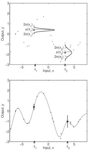
A Gaussian process is a collection of random variables which have a joint multivariate Gaussian distribution (Figure 1). Assuming a relationship of the formy=f(x)

between input x and output y, we have y1, . . . , yN ∼ N(0,Σ), where Σpq = Cov(yp, yq) =C(xp,xq) gives the covariance between output points corresponding to input points xp and xq. Thus, the mean µ(x) and the covariance functionC(xp,xq)fully specify the Gaussian process.

The value of covariance functionC(xp,xq)expresses the correlation between the individual outputs f(xp) and f(xq) with respect to inputs xp and xq. Note that the covariance function C(·,·) can be any function that generates a positive semi-definite covariance matrix. It is usually composed of two parts,

C(xp,xq) =Cf(xp,xq) +Cn(xp,xq), (2) whereCf represents the functional part and describes the unknown system we are modeling, andCnrepresents the noise part and describes the model of noise.

−5 0 5 −3 −2 −1 0 1 2 3 Input, x Output, y x 1 x2 µ(x 1) 2σ(x 1) 2σ(x 1) µ(x 2) 2σ(x 2) 2σ(x 2) −5 0 5 −3 −2 −1 0 1 2 3 Input, x Output, y x 1 x2

Figure 1. Modeling with GP: (a) Gaussian prediction at a new pointx1, conditioned on the training points (.); (b) the predictive mean together with its2_{σerror bars for two points,}

x2 that is close to the training points, andx1 that is more distant.

For noise part most commonly used is the constant covariance function. Choice of the covariance function for the functional part also depends on the stationarity of the process. Assuming stationary data most commonly used covariance function is the square exponential covariance function, on the contrary assuming non-stationary data the polynomial or its special case the linear covariance function (3) can be used.

C(xp,xq) = D

X

d=1

wd·xdp·xdq+δpqv0 (3) wherewdandv0 are the ’hyperparameters’ of the covari-ance function,D is the input dimension, andδpq = 1 if p=q and0 otherwise. Hyperparameters can be written as a vector Θ = [w1, . . . , wD, v0]T. Other forms and combinations of covariance functions suitable for various applications can be found in [12]. For a given problem, the hyperparameter values are learned using the data at hand. Expression δpqv0 models the noise, presumed as

white, while parameters wd indicate the importance of individual inputs: ifwd is zero or near zero, it means the inputs in dimensiondcontain little information and could possibly be neglected.

Consider a set of N D-dimensional input vectors

X = [x1,x2, . . . ,xN] and a vector of output data y =

[y1, y2, . . . , yN]T. Based on the data (X,y), and given a new input vector x∗_{, we wish to find the predictive}

distribution of the corresponding output y∗_{. Unlike in}

other models, there is no model parameter determination within a fixed model structure. In building such model, most of the effort consists oftuning the hyperparameters of the covariance function. The number of parameters to be optimized is small (D+ 1 for linear covariance func-tion), which means that optimization convergence might be faster than with parametric models and that the ’curse of dimensionality’, so common to black-box identification problems, is circumvented or at least decreased.

GP models can be easily utilized for regression calcu-lation. Based on training setX, a covariance matrixKof sizeN×N is determined. The aim is to find the distribu-tion of the corresponding outputy∗ _{for some new input}

vectorx∗_{= [x1(N+ 1), x2(N+ 1), . . . , xD(N+ 1)]}T_. For the collection of random variables

[y1, . . . , yN, y∗]T we can write:

[y, y∗_]T _{∼ N(0}

,K∗_{) (4)}

with the covariance matrix

K∗₌         K k(x∗₎ kT(x∗_{) k(x}∗₎         (5)

wherey= [y1, . . . , yN]T is anN×1 vector of training targets. The predictive distribution of the output for a new test input has normal probability distribution with mean and variance µ(y∗_{) =k(x}∗₎T_K−1 y, (6) σ2(y∗_{) =k(x}∗_)−k(x∗₎T_K−1 k(x∗_{), (7)} wherek(x∗_{) = [C(x1,x}∗_{), . . . , C(xN,x}∗_)]T _{is theN×1} vector of covariances between the test and training cases, andk(x∗_{) =C(x}∗_,x∗_{)is the covariance between the test}

input itself.

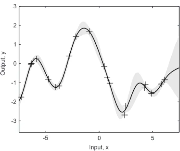
The obtained model, in addition to mean value, also provides information about the confidence in prediction by the variance. Usually, the confidence of the prediction is depicted with 2σ interval which is about 95% confi-dence interval. This conficonfi-dence region can be seen in the example in Figure 2 as a gray band. It highlights areas of the input space where the prediction quality is poor, due to the lack of data or noisy data, by indicating a wider confidence band around the predicted mean.

-5 0 5 0 1 2 3 Input, x Output, y -3 -2 -1

Figure 2. Using GP models: in addition to mean value (prediction), we obtain a 95% confidence region for the

underlying functionf (shown in gray).

To accurately reflect the correlations present in the training data, the hyperparameters of the covariance function need to be optimized. Due to the probabilistic nature of the GP models, the common model optimization approach where model parameters and possibly also the model structure are optimized through the minimization of a cost function defined in terms of model error (e.g. mean square error), is not readily applicable. A proba-bilistic approach to the optimization of the model is more appropriate. Actually, instead of minimizing the model error, the probability of the model is maximized.

The maximization of the probability of the model is usually done with maximum- likelihood estimation method. It can be restated as a cost function that is to be maximized. For numerical scaling purposes the log of the marginal likelihood is taken:

L(Θ) =−1 2log(|K|)− 1 2y T_K−1 y−N 2 log(2π). (8)

A frequently used method for optimizing the cost function is a conjugate gradients method. While this is a deterministic method, its result heavily depends on initial values of hyperparameters, especially for complex multidimensional systems, where the cost function has numerous local optima. Therefore a conjugate gradients method should be run repeatedly with various initial values of hyperparameters. As the space of possible values is huge, the initial values are often chosen randomly. Therefore, evolutionary algorithms can be considered as an alternative approach [16].

For modeling of time series we consider representation where the output at timetdepends on the delayed outputs y and the exogenous inputsu:

y(t) =f(y(t−1), . . . , y(t−n),

where ǫ(t) is white noise and the output y(t) depends on the state vectorx(t) = [y(t−1), y(t−2), . . . , y(t− n), u(t−1), u(t−2), . . . , u(t−n)]T _{at time stept.}

Assuming the signal is known up to t, we wish to predict the output of the system h steps ahead, i.e., we need to find the predictive distribution of y(t+h)

corresponding tox(t+h). Multiple-step-ahead predictions of a system modeled by (9) can be achieved by iteratively making repeated one-step-ahead predictions, up to the desired horizon [17], [18].

A noticeable drawback of system identification with GP models is the computation time necessary for the mod-eling. Regression based on GP models involves several matrix computations in which the load increases with the third power of the number of input data, such as matrix inversion and the calculation of the log-determinant of the used covariance matrix. This computational greed restricts the amount of training data, to at most a few thousand cases. To overcome the computational-limitation issues and to also make use of the method for large-scale dataset applications, numerous authors have suggested various sparse approximations [19], [20]. A common property to all sparse approximate methods is that they try to retain the bulk of the information contained in the full training dataset, but reduce the size of the resultant covariance matrix so as to facilitate a less computationally demanding implementation of the GP model.

IV. EXPERIMENTALRESULTS

To assess of the potential of GP models on financial data, the U.S. commodity markets data from [9] was chosen. The data consist of 11 futures markets in period from 2nd January 1990 to 9th August 2005:

1) Australian Dollar [AD] (Currency, CME) 2) British Pound [BP] (Currency, CME) 3) Cocoa [CC] (Soft, CSCE)

4) Canadian Dollar [CD] (Currency, CME) 5) Light Crude Oil [CL] (Energy, NYMEX) 6) Cotton [CT] (Grain, NYCE)

7) Feeder Cattle [FC] (Livestock, CME) 8) Gold [GC] (Metal, COMEX)

9) Heating Oil [HO] (Energy, NYMEX) 10) Gasoline [HU] (Energy, NYMEX) 11) Wheat [W] (Grain, CBOT)

Each of these markets has 33 information channels, but among these channels we have assumed only 7: opening, highest, lowest and closing prices, spot price, contango and backwardation. The goal is to predict the closing price of the futures contracts up to a horizon ofh= 14

days. The data at hand contained3,928trading days from which first1,000trading days are used to train the model and the rest of data is used for validation.

Regarding [9] future contracts usually are not traded for a period of 15 years. Therefore the time series had to be merged from data of more different contracts. The

time series used are synthesized as follows: the prices at the end of the trading period are real market prices and as we go back in time, when the active contract (the contract with the highest trade activity) changes, we switch to the previous active contract with price adjusted by an additive constant, so that there is no gap at the time of change. This way we create an artificial time series, which will differ from the time series of real prices. In the future this artificial transformation of data will be removed and the models will be used on a single contract time series.

As financial data is typically non-stationary and to be more fair in comparisson to BVAR models the linear co-variance function with automatic relevance determination is used for the functional part and the constant covariance function for the noise part. For modeling two types of training are used: offline and windowing. In the offline mode the model trained on the first 1,000 trading days is used forallpredictions, while in the windowing mode for eachprediction a new model is trained on preceding

1,000 trading days. Such a training should better catch local dependencies and adapt to market changes.

Both proposed models are compared to the BVAR model and the benchmark model described in [9]. Note that in our experiment no transformations are performed and no forgetting factors are used as well.

To measure the error of the prediction, the median relative error of the prediction is used,

MERE=median ˆ y(t+h) y(t+h)−1 . (10)

Hereyˆ(t+h)is the already mentioned point estimate of the price at time t+h andy(t+h) is real price at the same time. Median error is chosen for its robustness in the case of heavily outlying predictions.

Note that the predicted change in price is small com-pared to the price in vast majority of cases and especially in the cases with small prediction error. Therefore the ratio in MERE computation stays positive, so that it is a good measure of a relative error. Asymmetry between positive and negative relative error is neglected.

The obtained values of MERE (in parts per mille) for all markets and horizons h= 1, . . . ,14are summarized in Figure 3 as absolute differences where the basis (value 0) is the MERE value of the benchmark model. In other words, each horizon of each market is presented as a group of three columns. Red column presents online GP model (windowing), blue column presents offline GP model and green column presents BVAR model. Each col-umn presents absolute difference between corresponding model and benchmark model. Higher absolute difference means lower value of MERE, that is, better model, and vice versa.

From Figure 3 can be seen that there are markets (AD, CC, GC and W) where both GP models, trained online and offline, perform better than BVAR and benchmark model for all horizons, while in the case of the market

GP (windowing) GP (offline) BVAR (normal) -1 1 3 1 2 3 4 5 6 7 8 9 10 11 12 13 14 0 2 4 -1 1 3 -1 1 3 -2 0 2 4 -2 0 2 -1 1 3 5 -2 0 2 -2 0 2 AD BP CC CD CL CT FC GC HO HU W -2 0 2 4 -3 -1 1 3 5

Figure 3. Median relative error (shown in parts per mille [·10

3

]) computed for both, offline and online (windowing), GP models and normal BVAR models for horizons from 1 to 14. Results are compared to median realtive error of normal benchmark model

FC both models perform similar to BVAR model. On the other hand, there are markets (BP, CD, CL) where only online GP model (windowing) performs better than BVAR and benchmark model while offline GP model performs better than benchmark model and similar to BVAR model in lower horizons and worse than benchmark model in higher horizons. It seems that these markets have strong local dependencies, therefore model adaptation is neces-sary. Especially in the case of the market CD where offline GP model performs very poorly for higher horizons.

In the case of markets HO nad HU can be seen that both, online and offline, GP models are outperformed by BVAR model for all horizons and even by benchmark model for higher horizons. As it is concluded in [9] the reason could be low information value of the data channels used, which is in agreement with the EMH.

V. CONCLUSION

The results from our experimental work indicate that GP models are applicable to financial data as well as BVAR models are. GP models performed slightly better than BVAR models and benchmark models on major markets, specially in the case of online training with windowing which better catches local dependencies and adapts to market changes. On the other hand, GP models are outperformed by both, BVAR and benchmark, models on markets HO and HU. The reason for this could be low information value of the data channels used.

Among comparable results, the variance, which is ob-tained without additional computation and can be inter-preted as the measure of confidence in prediction, seems useful in the later decision making. Therefore GP models should be useful for applications where uncertainty can be taken into account.

Interesting further research might be investigation of correlations between markets. This could be done by merging all channels of all markets together and by using optimization with automatic relevance detection. In such a way influential channels would be neglected and therefore only important channels would be used. Although this might be huge computational load, by using modern hardware and paralellization we presume it could be done in a reasonable time.

REFERENCES

[1] E. Fama, “The beahvior of stock market prices,” Journal of Business, vol. 38, pp. 34–105, 1965.

[2] P. Samuelson, “Proof that properly anticipated prices fluctuate randomly,” Industrial Management Review, vol. 6, pp. 44–49, 1965.

[3] E. Fama, “Efficient capital markets: A review of theory and empirical work,”Journal of Finance, vol. 25, pp. 383–417, 1970. [4] L. Bachelier, “Theorie de la sp´eculation,”Paris: Gauthier-Villars, 1900, reprinted in P.H.Cootner: The Random Character of Stock Market Prices, 1964.

[5] E. Fama, “Efficient capital markets: II,”International Journal of Finance, vol. 46, pp. 1575–1617, 1991.

[6] C. Granger, “Forecasting stock market prices: Lessons for fore-casters,” International Journal of Forecasting, vol. 8, pp. 3–13, 1992.

[7] A. Timmerman and C. Granger, “Efficient market hypothesis and forecasting,”International Journal of Forecasting, vol. 20, pp. 15– 27, 2004.

[8] R. Litterman, “Forecasting with Bayesian vector autoregressions – five years of experience,” Journal of Business & Economic Statistics, vol. 4, pp. 25–38, 1986.

[9] J. ˇSindel´aˇr, “Study of BVAR(p) process applied to U.S. commod-ity market data,” World Academy od Science, Engineering and Technology, vol. 58, pp. 196–207, 2009.

[10] F. E. Tay and L. Cao, “Application of support vector machines in financial time series forecasting,”Omega, vol. 29, no. 4, pp. 309–317, 2001.

[11] K. Kim, “Financial time series forecasting using support vector machines,”Neurocomputing, vol. 55, no. 1-2, pp. 307–319, 2003. [12] C. E. Rasmussen and C. K. I. Williams,Gaussian Processes for

Machine Learning. The MIT Press, 2006.

[13] C. E. Rasmussen, “Advances in Gaussian processes,”Advances in Neural Information Processing Systems, 2006.

[14] M. Seeger, “Gaussian processes for machine learning,” Interna-tional Journal of Neural Systems, vol. 14, no. 2, pp. 69–106, 2004. [15] D. J. C. MacKay, “Introduction to Gaussian processes,”NATO ASI

Series, vol. 168, pp. 133–166, 1998.

[16] D. Petelin, B. Filipiˇc, and J. Kocijan, “Optimization of Gaussian process models with evolutionary algorithms,” 2011, submitted to 10th International Conference, ICANNGA 2011.

[17] J. Kocijan, A. Girard, B. Banko, and R. Murray-Smith, “Dynamic systems identification with Gaussian procesess,”Mathematical and Computer Modelling of Dynamic Systems, vol. 11, no. 4, pp. 411– 424, 2005.

[18] K. Aˇzman and J. Kocijan, “Application of Gaussian processes for black-box modelling of biosystems,” ISA Transactions, vol. 46, no. 4, pp. 443–457, 2007.

[19] J. Quinonero-Candela and C. E. Rasmussen, “A Unifying View of Sparse Approximate Gaussian Process Regression,”J. Mach. Learn. Res., vol. 6, pp. 1939–1959, 2005.

[20] J. Quinonero-Candela, C. E. Rasmussen, and C. K. I. Williams, “Approximation Methods for Gaussian Process Regression,” Mi-crosoft Research, Tech. Rep., September 2007.