University of Pennsylvania
ScholarlyCommons
Finance Papers Wharton Faculty Research
4-2017
Mispricing Factors
Robert F. Stambaugh
University of Pennsylvania
Yu Yuan
Follow this and additional works at:https://repository.upenn.edu/fnce_papers
Part of theFinance Commons, and theFinance and Financial Management Commons
This paper is posted at ScholarlyCommons.https://repository.upenn.edu/fnce_papers/163 For more information, please [email protected].
Recommended Citation
Stambaugh, R. F., & Yuan, Y. (2017). Mispricing Factors.The Review of Financial Studies, 30(4), 1270-1315.http://dx.doi.org/ 10.1093/rfs/hhw107
Mispricing Factors
Abstract
A four-factor model with two “mispricing” factors, in addition to market and size factors, accommodates a large set of anomalies better than notable four- and five-factor alternative models. Moreover, our size factor reveals a small-firm premium nearly twice usual estimates. The mispricing factors aggregate information across 11 prominent anomalies by averaging rankings within two clusters exhibiting the greatest return
co-movement. Investor sentiment predicts the mispricing factors, especially their short legs, consistent with a mispricing interpretation and the asymmetry in ease of buying versus shorting. A three-factor model with a single mispricing factor also performs well, especially in Bayesian model comparisons.
Disciplines
Mispricing Factors
Robert F. Stambaugh
The Wharton School, University of Pennsylvania and NBER
Yu Yuan
Shanghai Advanced Institute of Finance, Shanghai Jiao Tong University and
Wharton Financial Insitutions Center
First draft: July 4, 2015; this version: September 17, 2016 Forthcoming: Review of Financial Studies
A four-factor model with two “mispricing” factors, in addition to market and size factors, accommodates a large set of anomalies better than notable four- and five-factor alternative models. Moreover, our size factor reveals a small-firm premium nearly twice usual estimates. The mispricing factors aggregate information across 11 prominent anomalies by averaging rankings within two clusters exhibiting the greatest return co-movement. Investor sentiment predicts the mispricing factors, especially their short legs, consistent with a mispricing inter-pretation and the asymmetry in ease of buying versus shorting. A three-factor model with a single mispricing factor also performs well, especially in Bayesian model comparisons.
We are grateful for comments from Robert Dittmar, Robin Greenwood, Chen Xue, Lu Zhang, two anonymous referees, workshop participants at Chinese University of Hong Kong, Georgia State University, Hong Kong University, National University of Singapore, New York University, Purdue University, Shanghai Advanced Institute of Finance (SAIF), Singapore Management University, Southern Methodist University, University of Pennsylvania, and conference participants at the 2015 China International Conference in Finance, the 2015 Center for Financial Frictions Conference on Efficiently Inefficient Markets, the 2015 Miami Behavioral Finance Conference, the 2016 Q-Group Spring Seminar, the 2016 Research Affiliates Advisory Panel, the 2016 Society of Quantitative Analysts 50th Anniversary Conference, and the 2016 Symposium on Intelligent Investing at the Ivey Business School of the University of Western Ontario. We thank Mengke Zhang for excellent research assistance. Yuan gratefully acknowledges financial support from the NSF of China (71522012). Send correspondence to Yu Yuan, Shanghai Advanced Institute of Finance, Shanghai Jiao Tong University, 211 West Huaihai Road, Shanghai P.R.China, 200030, phone: +86-21-6293-2114, email: [email protected].
Modern finance has long valued models relating expected returns to factor sensitivities. A virtue of such models is parsimony. Once factors are constructed, the only additional data required to compute implied expected returns in standard applications are the historical returns on the assets being analyzed. Moreover, the number of factors has typically been small. For many years only a single market factor was popular, following the CAPM of Sharpe (1964) and Lintner (1965). Fama and French (1993) spurred widespread use of three factors, motivated by violations of the single-factor CAPM related to firm size and value-versus-growth measures.
Numerous studies have identified anomalies that violate the three-factor model, but only occasionally have anomalies contended for status as additional factors, given the virtue of parsimony in a factor model.1
Given the proliferation of anomalies, however, the need for an alternative factor model that can accommodate more anomalies has become increasingly clear. Two additional factors have recently received significant attention. Hou, Xue, and Zhang (2015a) propose a four-factor model that combines market and size factors with two new factors based on investment and profitability. Fama and French (2015) add somewhat different versions of investment and profitability factors to their earlier three-factor model (Fama and French (1993)), creating a five-factor model. Both studies provide theoretical motivations for why these factors contain information about expected return: Hou, Xue, and Zhang (2015a) rely on an investment-based pricing model, while Fama and French (2015) invoke comparative statics of a present-value relation. At the same time, it should be noted that both investment and profitability are two of the numerous anomalies documented earlier in the literature.2
In subsequent studies, Fama and French (2016) and Hou, Xue, and Zhang (2015b) examine their models’ abilities to explain other anomalies.
We take a different approach to factor construction. Instead of having a factor correspond to a single anomaly, we combine the information in multiple anomalies. Clearly an important dimension on which a parsimonious factor model is judged is its ability to accommodate a wide range of anomalies. Our approach exploits that range when forming the factors. Rather than construct a factor using stocks’ rankings on a single anomaly variable, such as investment, we construct a factor by averaging rankings across multiple anomalies. By averaging, we aim to achieve a less noisy measure of a stock’s mispricing, thereby identifying
1
A notable example subsequent to Fama and French (1993) is the momentum anomaly documented by Jegadeesh and Titman (1993), which motivates the frequently used momentum factor proposed by Carhart (1997).
2
Titman, Wei, and Xie (2004) and Xing (2008) show that high investment predicts abnormally low returns, while Fama and French (2006), Chen, Novy-Marx, and Zhang (2010), and Novy-Marx (2013) show that high profitability predicts abnormally high returns.
more precisely which stocks to long and which stocks to short when constructing a factor that can better accommodate anomalies reflecting mispricing.
We apply our approach by constructing two factors from the set of 11 prominent anomalies examined by Stambaugh, Yu, and Yuan (2012, 2014, 2015). In constructing the factors, we average rankings within two clusters of anomalies formed by grouping together the anomalies exhibiting the greatest similarity. We can measure similarity either by time-series correlations of anomalies’ long-short return spreads or by cross-sectional correlations of stocks’ rankings on the anomaly variables. Both measures yield the same two clusters of anomalies. The two mispricing factors are then combined with market and size factors to obtain a four-factor model.
Our model’s overall ability to accommodate anomalies exceeds that of both the four-factor model of Hou, Xue, and Zhang (2015a) and the five-four-factor model of Fama and French (2015). This conclusion obtains not only within the set of anomalies used to construct the factors but also for the substantially larger set of 73 anomalies examined previously by Hou, Xue, and Zhang (2015a, 2015b). For example, when applied to the 51 of those anomalies having data over our entire sample period, the Gibbons-Ross-Shanken (1989) test of whether all the anomalies’ alphas equal zero produces a p-value of 0.10 for our model compared to 0.003 or less for these four- and five-factor alternative models. Our model also performs better than these alternatives when the models are judged by their abilities to explain each other’s factors. As discussed by Barillas and Shanken (2015a, 2015b), judging factor models this way is implied by standard model-comparison procedures, under both frequentist and Bayesian approaches. We apply both approaches in our comparisons.
We also construct a three-factor model by replacing our two mispricing factors with a single factor that averages rankings across the entire set of 11 anomalies, rather than within two clusters in that set. When models are again judged by their abilities to explain each other’s factors, this three-factor model outperforms the four-factor model of Hou, Xue, and Zhang (2015a) and the five-factor model of Fama and French (2015). It also outperforms the latter model in explaining anomalies.
Our size factor is constructed using stocks least likely to be mispriced, as identified by the measures used to construct our mispricing factors. Our resulting SMB delivers a small-firm premium of 46 bps per month over our 1967–2013 sample period, nearly twice the premium of 25 bps implied by the familiar SMB factor in the Fama-French three-factor model. Consistent with mispricing exerting less effect on our size three-factor, the investor sentiment index of Baker and Wurgler (2006) exhibits significant ability to predict the
Fama-FrenchSMB but not our SMB.
The basic concepts motivating our approach are that anomalies in part reflect mispricing and that mispricing has common components across stocks. Both concepts are consistent with previous evidence. As we discuss, a large empirical literature links anomalies to mispric-ing, and numerous studies find pervasive effects often characterized as investor sentiment. By combining information across anomalies, we aim to construct factors capturing common elements of mispricing. Consistent with this intent, we find that investor sentiment predicts our mispricing factors, especially their short legs. The stronger predictability of the short legs is consistent with asymmetry in the ease of buying versus shorting (e.g., Stambaugh, Yu, and Yuan (2012)).
Factor models can be useful whether expected returns reflect risk or mispricing. Factors can capture systematic risks for which investors require compensation, or they can cap-ture common sources of mispricing, such as market-wide investor sentiment. This point is emphasized, for example, by Hirshleifer and Jiang (2010) and Kozak, Nagel, and Santosh (2015). Moreover, there need not be a clean distinction between mispricing and risk com-pensation as alternative motivations for factor models of expected return. For example, DeLong, Shleifer, Summers, and Waldman (1990) explain how fluctuations in market-wide “noise-trader” sentiment create an additional source of systematic risk for which rational traders require compensation.
When expected returns reflect mispricing and not just compensation for systematic risks, some of the mispricing may not be driven by pervasive sentiment factors but may instead be asset specific, as discussed for example by Daniel and Titman (1997). In that sense the concept of “mispricing factors” potentially embeds some inconsistency. On the other hand, previous studies discussed below do find that mispricing appears to exhibit commonality across stocks. The extent to which our factors help describe expected returns is an empirical question. A parsimonious factor model that outperforms feasible alternatives seems useful from a practical perspective, as no model can be entirely correct.
One practical use of factor models, in addition to explaining expected returns, is to capture systematic time-series variation in realized returns. We also examine the extent to which our mispricing factors can perform this role as compared to the factors in the alternative models we consider. Our results indicate that the ability of mispricing factors to explain expected returns better (i.e., to accommodate amomalies better) does not come at the cost of sacrificing ability to capture return variance.
The remainder of the paper proceeds as follows. Section 1 briefly discusses the consid-erable evidence linking anomalies to mispricing and to pervasive sentiment effects. Section 2 explains the construction of our two mispricing factors and our size factor and examines their empirical properties. The resulting four-factor model is compared to notable alterna-tive factor models in Section 3. Section 4 considers a model with just a single mispricing factor. Section 5 illustrates a shared limitation of the factor models, showing how they can seem to explain the idiosyncratic volatility puzzle if the role of mispricing is not considered. Section 6 reviews our conclusions.
1.
Anomalies, Mispricing, and Sentiment
Much of the return-anomaly literature, too extensive for us to survey comprehensively, points to mispricing as being at least partially responsible for the documented anomalous returns. We base our mispricing factors on a prominent subset of the many anomalies reported in the literature, and, within this subset, studies containing mispricing interpretations include Ritter (1991) for net stock issues, Daniel and Titman (2006) for composite equity issues, Sloan (1996) for accruals, Hirshleifer, Hou, Teoh, and Zhang (2004) for net operating as-sets, Cooper, Gulen, and Schill (2008) for asset growth, Titman, Wei, and Xie (2004) for investment-to-assets, Campbell, Hilscher, and Szilagyi (2008) for financial distress, Jegadeesh and Titman (1993) for momentum, and Wang and Yu (2013) for profitability anomalies in-cluding return on assets and gross profitability. A mispricing interpretation of anomalies is also consistent with the evidence of McLean and Pontiff (2015), who observe that fol-lowing an anomaly’s academic publication, there is greater trading activity in the anomaly portfolios, and anomaly profits decline.
Idiosyncratic volatility (IVOL) represents risk that deters price-correcting arbitrage. This concept is advanced, for example, by DeLong, Shleifer, Summers, and Waldman (1990), Pontiff (1996), Shleifer and Vishny (1997), and Stambaugh, Yu, and Yuan (2015). One should therefore expect stronger anomaly returns among stocks with higher IVOL. Studies finding that various return anomalies are indeed stronger among high-IVOL stocks include Pontiff (1996) for closed-end fund discounts, Wurgler and Zhuravskaya (2002) for index inclusions, Mendenhall (2004) for post-earnings announcement drift, Ali, Hwang, and Trombley (2003) for the value premium, Zhang (2006) for momentum, Mashruwala, Rajgopal, and Shevlin (2006) for accruals, Scruggs (2007) for “Siamese twin” stocks, Ben-David and Roulstone (2010) for insider trades and share repurchases, McLean (2010) for long-term reversal, Li
and Zhang (2010) for asset growth and investment to assets, Larrain and Varas (2013) for equity issuance, and Wang and Yu (2013) for return on assets.
As explained by Stambaugh, Yu, and Yuan (2015), if there is less arbitrage capital available to short overpriced stocks than to purchase underpriced stocks, then the effect of IVOL should be larger among overpriced stocks. Jin (2013) examines ten anomaly long-short spreads and finds all to be more profitable among high-IVOL stocks than among low-IVOL stocks, and this difference is attributable primarily to the short leg of each spread. Stambaugh, Yu, and Yuan (2015) find, consistent with arbitrage risk and mispricing, that the IVOL-return relation is negative among overpriced stocks but positive among underpriced stocks, with mispricing determined by combining the same 11 return anomalies used in this study. Moreover, those authors find that the negative IVOL-return relation among overpriced stocks is stronger than the positive relation among underpriced stocks, consistent with the arbitrage asymmetry in buying versus shorting.
When mispricing is present, stocks that are more difficult to short should also be those for which overpricing is less easily corrected. Evidence that short-leg profits of anomaly long-short spreads are indeed greater among stocks with greater shorting impediments is provided by Nagel (2005), Hirshleifer, Teoh, and Yu (2011), Avramov, Chordia, Jostova, and Philipov (2013), Drechsler and Drechsler (2014), and Stambaugh, Yu, and Yuan (2015). The last study also shows that the negative IVOL-return relation among overpriced stocks is stronger among stocks less easily shorted.
Evidence consistent with a common sentiment-related component of mispricing is pro-vided, for example, by Baker and Wurgler (2006) and Stambaugh, Yu, and Yuan (2012).3
The latter study finds that the short-leg returns for long-short spreads associated with each of 11 anomalies we use in this study are significantly lower following a high level of investor sentiment as measured by the Baker-Wurgler sentiment index. Stambaugh, Yu, and Yuan (2015) find that the negative (positive) IVOL-return relation among overpriced (underpriced) stocks is stronger following a high (low) level of the Baker-Wurgler index, consistent with arbitrage risk deterring the correction of sentiment-related mispricing.
This study’s objective is not to make a case for the presence of mispricing in the stock market. For that we rely on the previous literature discussed above. We do, however, provide two novel results with regard to the role of investor sentiment, as will be discussed later. First, investor sentiment predicts our mispricing factors, particularly their short (overpriced)
3
Baker, Wurgler, and Yuan (2012) find that sentiment-related effects similar to those documented in the U.S. by Baker and Wurgler (2006) also occur in a number of other countries.
legs. Second, unlike the size factor constructed by Fama and French (1993), our size factor— constructed to be less contaminated by mispricing—is not predicted by sentiment.
2.
Anomalies and Factors
Our objective is to explore parsimonious factor models that include factors combining in-formation from a range of anomalies. We first construct a four-factor model that includes two mispricing factors along with market and size factors. Later we consider a three-factor model with just a single mispricing factor.
The first factor in our four-factor model is the excess value-weighted market return, stan-dard in essentially all factor models with pre-specified factors. Constructing the remaining three factors—a size factor and two mispricing factors—involves averaging stocks’ rankings with respect to various anomalies. We use the same 11 anomalies analyzed by Stambaugh, Yu, and Yuan (2012, 2014, 2015). While the number of anomalies used to construct the factors could be expanded, we use this previously specified set to alleviate concerns that a different set was chosen to yield especially favorable results for this study. The Appendix provides brief descriptions of the 11 anomalies: net stock issues, composite equity issues, accruals, net operating assets, asset growth, investment-to-assets, distress, O-score, momen-tum, gross profitability, and return on assets.
Rather than constructing a five-factor model by adding our two mispricing factors to the three factors of Fama and French (1993), we opt for only four factors. That is, we do not include a book-to-market factor and instead include only a size factor in addition to the market and our mispricing factors. Our motivation here is parsimony and long-standing evidence that firm size is related not only to average return but also to a number of other stock characteristics such as volatility, liquidity, and sensitivities to macroeconomic conditions.4
Not including a factor based on book-to-market reflects the literature’s less settled view of that variable’s role and importance. As we report later, our mispricing factors price the book-to-market factor, suggesting our decision to exclude a book-to-market factor is reasonable.
4
For example, see Banz (1981) on average return, Amihud and Mendelson (1989) on volatility and liq-uidity, and Chan, Chen, and Hsieh (1985) on sensitivities to macroeconomic conditions.
2.1.
The Mispricing Factors
We construct factors based on averages of stocks’ anomaly rankings. This approach is easily motivated. Letα denote a non-zero vector of alphas for a universe of stocks with respect to a benchmark factor, P.5
That is, α is the intercept vector in the multivariate regression
rt=α+βrP,t+t, (1)
where rt is the vector containing the stocks’ excess returns in period t, and rP,t is the
benchmark’s excess return. Consider a factorQwith returnrQ,t =w0rt, wherewis a weight
vector. Suppose that adding rQ,t to the right-hand side of (1) leaves no remaining alphas.
That is, the resulting regression becomes
rt = Θ " rP,t rQ,t # +ηt. (2)
If this additional factor can also produce a covariance matrix for ηt of the form σ2I, then
setting w proportional to α produces the desired Q, as shown by MacKinlay and P´astor (2000).6
In other words, the additional factor that completes the pricing job is constructed by going long stocks with positive alphas and short stocks with negative alphas. Our approach to this long-short construction ofQessentially treats each stock’s cross-sectional ranking with respect to an anomaly as a noisy proxy for the stock’s alpha ranking. Some of that noise is diversified away by averaging rankings across anomalies, thereby more precisely indicating which stocks to buy and which stocks to short when constructing the factor. Excluding stocks from the middle of the average-ranking distribution, as we do, further increases the likelihood of making correct long/short classifications when constructing the factor. We term the resulting factor corresponding to Q a “mispricing” factor, reflecting our view, discussed earlier, that mispricing is an important element of anomaly-related alphas.
Our approach based on averaging anomaly rankings stands in contrast to previous ap-proaches that construct a factor by ranking on a single variable that initially gained attention as a return anomaly. If such a variable is uniquely motivated as capturing either a systematic-risk sensitivity or mispricing, then our approach simply contaminates that variable with ex-traneous information. On the other hand, if that variable is not so uniquely valuable, then our approach can work better. Our empirical results support the latter scenario.
5
Assuming a single-factor benchmark is essentially without loss of generality, asP can be viewed as the maximum-Sharpe-ratio combination of multiple factors.
6
Those authors show that when the unique portfolioZ that is orthogonal toP and produces zero alphas also produces a scalar covariance matrix of residuals, then Z is a combination ofP and a portfolio whose weights are proportional toα, as are the weights inQ. (See in particular their equation 26 on page 891.) Regressing rt on rP,t and rZ,t therefore produces the same residuals and (zero) intercept vector as does
As noted earlier, we construct mispricing factors by averaging rankings within the set of 11 prominent anomalies examined by Stambaugh, Yu, and Yuan (2012, 2014, 2015). The initial step in constructing two mispricing factors is to separate the 11 anomalies into two clusters, with a cluster containing the anomalies most similar to each other. Similarity can be measured by either of two methods, using either time-series correlations of anomaly returns or average cross-sectional correlations of anomaly rankings. Both methods produce the same two clusters of anomalies.
In the first method, for each anomaly i we compute the spread, Ri,t, between the
value-weighted returns in month t on stocks in the first and tenth NYSE deciles of the ranking variable in a sort at the end of montht−1 of all NYSE/AMEX/NASDAQ stocks with share prices greater than $5, where the ordering produces a positive estimated intercept in the regression
Ri,t=αi+biMKTt+ciSMBt+ui,t, (3)
and MKTt and SMBt are the market and size factors constructed by Fama and French
(1993).7
Next we compute the correlation matrix of the estimated residuals in equation (3). Our sample period runs from January 1967 through December 2013, except data for the distress anomaly begin in October 1974, and data for the return-on-assets anomaly begin in November 1971. To deal with the heterogeneous starting dates, we compute the correlation matrix using the maximum likelihood estimator analyzed by Stambaugh (1997). Using this correlation matrix, we form two clusters by applying the same procedure as Ahn, Conrad, and Dittmar (2009), who combine a correlation-based distance measure with the clustering method of Ward (1963).8
In the second method, we compute the z-score of each stock’s ranking percentile for each anomaly and then compute the cross-sectional correlations between the z-scores for all available pairs of the 11 anomalies. This procedure gives a set of correlations each month, and we average these correlations across the months in our sample period. The resulting 11 ×11 matrix of average correlations is then used to form two clusters using the same
7
For the anomaly variables requiring Compustat data from annual financial statements, we require at least a four-month gap between the end of montht−1 and the end of the fiscal year. When using quarterly reported earnings, we use the most recent data for which the reporting date provided by Compustat (item RDQ) precedes the end of montht−1. When using quarterly items reported from the balance sheet, we use those reported for the quarter prior to quarter used for reported earnings. The latter treatment allows for the fact that a significant number of firms do not include include balance-sheet information with earnings announcements and only later release it in 10-Q filings (see Chen, DeFond, and Park (2002)). For anomalies requiring return and market capitalization, we use data recorded for montht−1 and earlier, as reported by CRSP.
8
Using the version of SM B we construct later in subsection 2.2, instead of the Fama-French version of SM B, does not change any of our cluster-identification results.
procedure applied above to the correlation matrix of long-short returns.
The first cluster of anomalies includes net stock issues, composite equity issues, accruals, net operating assets, asset growth, and investment to assets. These six anomaly variables all represent quantities that firms’ managements can affect rather directly. Thus, we denote the factor arising from this cluster asMGMT. (The factor construction is described below.) The second cluster includes distress, O-score, momentum, gross profitability, and return on assets. These five anomaly variables are related more to performance and less directly controlled by management, so we denote the factor arising from this cluster as P ERF. Although we assign names to the clusters, we do not suggest that a cluster reflects a single behavioral story. For example, within the MGMT cluster, equity issuance anomalies could reflect managerial action triggered by mispricing (e.g., Daniel and Titman (2006)), while asset growth and investment anomalies could reflect mispricing triggered by managerial action (e.g., Cooper, Gulen, and Schill (2008)). Moreover, even within the issuance anomalies, multiple effects could be at work, as the results of Greenwood and Hanson (2012) suggest. While there may exist unifying behavioral themes underlying the identities of our clusters, discovering such a framework is beyond the scope of our study.
We next average a stock’s rankings with respect to the available anomaly measures within each of the two clusters. Thus, each month a stock has two composite mispricing measures,
P1 andP2. Our averaging of anomaly rankings closely follows the approach of Stambaugh, Yu, and Yuan (2015), who construct a single composite mispricing measure by averaging across all 11 anomalies.9
As in that study, we equally weight a stock’s rankings across anomalies—a weighting that is simple, transparent, and not sample-dependent. As dis-cussed earlier, the rationale for averaging is that, through diversification, a stock’s average rank yields a less noisy measure of its mispricing than does its rank with respect to any single anomaly. The evidence suggests that such diversification is effective. As observed by Stambaugh, Yu, and Yuan (2015), the spread between the alphas for portfolios of stocks in the top and bottom deciles of the average ranking across the 11 anomalies is nearly twice the average across those anomalies of the spread between the top- and bottom-decile alphas of portfolios formed using an individual anomaly (with alphas computed using the three-factor model of Fama and French (1993)). We verify a similar result in our sample: The former spread is 95 basis points per month while the latter spread is 53 basis points, and the difference of 42 basis points has a t-statistic of 3.80.
9
Stambaugh, Yu, and Yuan (2015) also report a robustness exercise that employs a clustering approach similar to that reported above.
We construct the mispricing factors by applying a 2×3 sorting procedure resembling that of Fama and French (2015). The approach in that study generalizes the approach in Fama and French (1993), and a similar procedure is applied in Hou, Xue, and Zhang (2015a). Specifically, each month we sort NYSE, AMEX, and NASDAQ stocks (excluding those with prices less than $5) by size (equity market capitalization) and split them into two groups using the NYSE median size as the breakpoint. Independently, we sort all stocks by P1 and assign them to three groups using as breakpoints the 20th and 80th percentiles of the combined NYSE, AMEX, and NASDAQ universe. We similarly assign stocks to three groups according to sorts on P2. To construct the first mispricing factor, MGMT, we compute value-weighted returns on each of the four portfolios formed by the intersection of the two size categories with the top and bottom categories forP1. The value of MGMT for a given month is then the simple average of the returns on the two low-P1 portfolios (underpriced stocks) minus the average of the returns on the two high-P1 portfolios (overpriced stocks). The second mispricing factor, P ERF, is similarly constructed from the low- and high-P2 portfolios.
The persistence of the measures used to construct our mispricing factors is similar to that of measures used to form other familiar factors. A simple gauge of persistence is the time-series average of the cross-sectional correlation between a given measure’s rankings in adjacent months. This average correlation equals 0.955 and 0.965 for the composite mispricing measures used to construct MGMT and P ERF. The measures used to form the book-to-market, investment, and profitability factors in Fama and French (2015) have average rank correlations of 0.983, 0.943, and 0.981, respectively. Hou, Xue, and Zhang (2015a) construct essentially the same investment factor, while their somewhat different profitability factor uses a measure whose average rank correlation is 0.883. In comparison, market capitalization of equity, used to construct the size factors in all of the above models, has an average rank correlation of 0.996.
One might note that for the breakpoints of P1 and P2, we use the 20th and 80th per-centiles of the NYSE/AMEX/NASDAQ, rather than the 30th and 70th perper-centiles of the NYSE, used by the studies cited above that apply a similar procedure to different variables. These modifications reflect the notion that relative mispricing in the cross-section is likely to be more a property of the extremes than of the middle. Stambaugh, Yu, and Yuan (2015) find, for example, that the negative (positive) effects of idiosyncratic volatility for overpriced (underpriced) stocks are consistent with the role of arbitrage risk deterring the correction of mispricing, and those authors show that such effects occur primarily in the extremes of a composite mispricing measure and are stronger for smaller stocks. Subsection 3.4 explains
that our main results are robust to the various deviations we take from the more conventional factor-construction methodology tracing to Fama and French (1993). The online appendix reports detailed results of those robustness checks.
Table 1 presents means, standard deviations, and correlations for monthly series of the four factors in our model. (The construction of our size factor, SMB, is explained below.) We see that the two mispricing factors, MGMT and P ERF, have zero correlation with each other (to two digits) in our overall 1976–2013 sample period. That is, the clustering procedure, coupled with the averaging of individual anomaly rankings, essentially produces two orthogonal factors.
2.2.
The Size Factor
When constructing our size factor, we depart more significantly from the approach in Fama and French (2015) and other studies cited above. The stocks we use to form the size factor in a given month are the stocks not used in forming either of the mispricing factors. Specifically, to construct our size factor, SMB (small minus big—that notation we keep), we compute the return on the small-cap leg as the value-weighted portfolio of stocks present in the intersection of both small-cap middle groups when sorting on P1 and P2. Similarly, the large-cap leg is the value-weighted portfolio of stocks in the intersection of the large-cap middle groups in the sorts on the mispricing measures. The value ofSMB in a given month is the return on the small-cap leg minus the large-cap return.
Each 2×3 sort on size and one of the mispricing measures produces six categories, so in total twelve categories result from the sorts using each of the two mispricing measures. If we were to follow the more familiar approach of Fama and French (2015) and others, we would compute SMB as the simple average of the value-weighted returns on the six small-cap portfolios minus the corresponding average of returns on the six large-small-cap portfolios. By averaging across the three mispricing categories, that approach would seek to neutralize the effects of mispricing when computing the size factor. The problem is that such a neutraliza-tion can be thwarted by arbitrage asymmetry—a greater ability or willingness to buy than to short for many investors. With such asymmetry, the mispricing within the overpriced category is likely to be more severe than the mispricing within the underpriced category. Moreover, this asymmetry is likely to be greater for small stocks than for large ones, given that small stocks present potential arbitrageurs with greater risk (e.g., idiosyncratic
volatil-ity).10
Thus, simply averaging across mispricing categories would not neutralize the effects of mispricing, and the resultingSMBwould have an overpricing bias. This bias is a concern not just when sorting on our mispricing measures but when sorting on any measure that is potentially associated with mispricing. Some studies argue that book-to-market, for exam-ple, contains a mispricing effect (e.g., Lakonishok, Shleifer, and Vishny (1994)), so one might raise a similar concern in the context of the version of SMB computed by Fama and French (1993). By instead computing SMB using stocks only from the middle of our mispricing sorts, avoiding the extremes, we aim to reduce this effect of arbitrage asymmetry.
Consistent with the above argument, our approach delivers a small-cap premium that significantly exceeds not only the value produced by the above alternative method but also the small-cap premium implied by the version ofSMB in the three-factor model of Fama and French (1993). For our sample period of January 1967 through December 2013, our SMB
factor has an average of 46 bps per month. In contrast, the alternative method discussed above gives an SMB with an average of 28 bps, close to the average of 25 bps for the three-factor Fama-French version ofSMB. The differences between our estimated small-cap premium and these alternatives are significant not only statistically (t-statistics: 3.99 and 4.19) but economically as well, indicating a size premium that is nearly twice that implied by the familiar Fama-French version ofSMB. This result is similar to the conclusion of Asness, Frazzini, Israel, Moskowitz, and Pedersen (2015), who find that the size premium becomes substantially greater when controlling for other stock characteristics potentially associated with mispricing. Those authors conclude that explaining a significant size premium presents a challenge to asset pricing theory. Such a challenge is beyond the scope of our study as well. Even though the size premium is a fundamentally important quantity, our comparison below of factor models’ abilities to explain anomalies is not sensitive to the method used to construct the size factor. (We present further discussion and evidence of this point in subsection 3.4 and in the online appendix.)
Our procedure also appears to have minimal effect on the distribution of firm sizes used in computing SMB. For example, if we first compute the value-weighted average of log size (with size in $1000) for the six small-cap portfolios described above in the more familiar approach, and we then take the simple average of those six values (analogously to what is done with returns), the result is 12.28. If we instead compute the value-weighted average of log size for the firms in the small-cap leg of our SMB, the result is 12.31, nearly identical. The same comparison for large firms gives 15.81 for the more familiar approach versus 15.83 for the firms in the large-cap leg of ourSMB.
10
One might ask whether the same approach we take in constructing the size factor— excluding stocks more likely to be mispriced—matters for constructing other factors as well. For example, one could follow this approach when constructing a book-to-market factor. We explore this question for that factor in particular and do find a substantial effect. Specifically, we separate stocks into six groups, following the same procedure as Fama and French (1993), but then before computing value-weighted returns within each group and forming the HML factor, we delete the stocks in the top 20% and bottom 20% of either of our mispricing measures. This additional step renders the value premium 40 percent smaller and statistically insignificant.11
2.3.
Factor Betas, Arbitrage Asymmetry, and Sentiment Effects
Table 2 gives parameter estimates from our four-factor model for the individual long-short strategies based on the anomaly measures used above as well as book-to-market. Panel A contains the alphas and factor sensitivities (“betas”) of the long-short spreads between the value-weighted portfolios of stocks in the long leg (bottom decile) and short leg (top decile). Panel B gives corresponding estimates for the long legs, and Panel C reports estimates for the short legs. The breakpoints are based on NYSE deciles, but all NYSE/AMEX/NASDAQ stocks with share prices of at least $5 are included.12
For anomalies in the first cluster, the long-short betas on the first mispricing factor,MGMT, are positive witht-statistics between 6.09 and 18.12, whereas the same anomalies’ long-short betas on the second factor, P ERF, are uniformly lower and havet-statistics of mixed signs that average just 1.27. Similarly, for anomalies in the second cluster, the long-short betas onP ERF are positive witht-statistics between 5.02 and 24.10, while the betas on MGMT have mixed-sign t-statistics averaging −0.17. These results confirm that averaging anomaly rankings within a cluster produces a factor that captures common variation in returns for the anomalies in that cluster. Not surprisingly, for each anomaly with respect to its corresponding factor, the short-leg beta is significantly negative and the long-leg beta is significantly positive, with the long leg for accruals being the only exception.
Also observe in Table 2 that the short-leg betas are generally larger in absolute magnitude than their long-leg counterparts. With the first-cluster anomalies, for example, the average short-legMGMT beta is−0.46, whereas the average long-legMGMT beta is 0.20. Similarly,
11
For our sample period, the monthly average of this alternative book-to-market factor is 0.22% with a t-statistic of 1.81, whereas the Fama-French HML factor has an average of 0.37% with at-statistic of 3.01.
12
NYSE breakpoints are also used, for example, by Fama and French (2016) and Hou, Xue, and Zhang (2015a).
for the second-cluster anomalies, the short-leg P ERF betas average −0.49 as compared to 0.30 for the long legs. If the factors indeed capture systematic components of mispricing, a greater short-leg sensitivity is consistent with the arbitrage asymmetry discussed above. This arbitrage asymmetry leaves more uncorrected overpricing than uncorrected underpricing, implying greater sensitivity to systematic mispricing for overpriced (short-leg) stocks than for uncerpriced (long-leg) stocks.
Arbitrage asymmetry is also consistent with the relation between investor sentiment and anomaly returns. For each of the anomalies we use to construct our factors, Stambaugh, Yu, and Yuan (2012) observe that the short leg of the long-short anomaly spread is significantly more profitable following high investor sentiment, whereas the long-leg profits are less sen-sitive to sentiment. We observe similar sentiment effects for our mispricing factors. Table 3 reports the results of regressing each factor as well as its long and short legs on the previous month’s level of the investor sentiment index of Baker and Wurgler (2006).13
For the two mispricing factors, MGMT and P ERF, the slope coefficients on both the long and short legs are uniformly negative, consistent with sentiment effects, but the slopes for the short legs are two to three times larger in magnitude. The short-leg coefficients for the two factors are nearly identical, as are the t-statistics of −2.06 and −2.05. The long-leg t-statistics, in contrast, are just −0.98 and−1.29.
The stronger sentiment effects for the short legs ofMGMT andP ERF can be understood in the context of the study by Stambaugh, Yu, and Yuan (2012), who find that the short-leg returns of each of the same 11 anomalies used here are significantly lower following high sentiment. Unlike that study’s long-short spreads, MGMT and P ERF reflect average anomaly rankings and include more than just the top and bottom deciles, but it is not surprising our results are nevertheless similar. As that study explains, given that many investors are less willing or able to short stocks than to buy them, overpricing resulting from high investor sentiment gets corrected less by arbitrage than does underpricing resulting from low sentiment. Sentiment therefore exhibits a stronger relation to short-leg anomaly returns than to long-leg returns. The significantly positive t-statistics in Table 3 for the sentiment sensitivity of each long-short difference (i.e., each mispricing factor) confirm the greater sentiment effect on the short-leg returns. Overall, the long-short asymmetry in factor betas (Table 2) and sentiment effects (Table 3) is consistent with a mispricing interpretation of our factors.
13
Because investor sentiment can be correlated with economic conditions (e.g., investors can be excessively optimistic when times are good), we use the raw sentiment index produced by Baker and Wurgler (2006) rather than version they orthogonalize with respect to macro factors.
Sentiment does not exhibit much ability to predict our size factor. In Table 3, the t -statistic is −1.60 for the slope coefficient when regressing the long-short spread (SMB) on lagged sentiment, and the t-statistics for the long and short legs (small and large firms) are −1.72 and −1.17. If sentiment affects prices, then periods of high (low) sentiment are likely to be followed by especially low (high) returns on overpriced (underpriced) stocks, especially among smaller stocks, which are likely to be more susceptible to mispricing. Baker and Wurgler (2006) report evidence consistent with this hypothesis, which implies a negative relation between lagged sentiment and the return on a spread that is long small stocks and short large stocks—if mispriced stocks are included, especially in the small-stock leg. The lack of a significant relation between our SMB factor and sentiment suggests some success in our attempt to avoid mispriced stocks when constructing the factor. In contrast, for example, sentiment does exhibit a significant ability to predict the familiar SMB factor from the three-factor model of Fama and French (1993). The slope coefficient is nearly 50% greater in magnitude (−0.32 versus −0.22) and has a t-statistic of −2.31. In fact, the t -statistic for the difference in slopes of −0.10 is−1.68, which is significant at the 5% level for the one-tailed test implied by the alternative hypothesis that ourSMB factor is less affected by mispricing.
Our labeling of MGMT and P ERF as “mispricing” factors is not what distinguishes them from factors in other models. For example, the investment and profitability factors in the models of Fama and French (2015) and Hou, Xue, and Zhang (2015a) can also reflect mispricing. While both of those studies provide models linking investment and profitability to expected return, their models do not distinguish rational risk-based compensation versus mispricing as the source of expected return. The latter could well be at work: when the short-leg returns of those factors (two from each study) are regressed on lagged investor sentiment, thet-statistics lie between−1.93 and −2.36, consistent with both the results and mispricing interpretation in Stambaugh, Yu, and Yuan (2012). As explained earlier, what instead distinguishes our factors is that they are based on combining the information in multiple anomalies, as opposed to being single-anomaly factors.
3.
Comparing Factor Models
Fama and French (2016) explore the ability of the five-factor model of Fama and French (2015) to accommodate various return anomalies. Hou, Xue, and Zhang (2015b) compare that model to the four-factor model of Hou, Xue, and Zhang (2015a) by investigating the two
models’ abilities to explain a range of anomalies. We evaluate our four-factor model relative to both of those models, also including the three-factor model of Fama and French (1993) in the comparison as a familiar benchmark.14
In subsection 3.1, we compare the models’ relative abilities to explain a range of individual anomalies, both the set of 12 anomalies examined in Table 2 as well as the substantially wider set of 73 anomalies analyzed by Hou, Xue, and Zhang (2015a, 2015b). Subsection 3.2 then reports pairwise model comparisons that evaluate each model’s ability to explain factors present in another. Subsection 3.3 compares models using Bayesian posterior model probabilities. Results of robustness investigations are summarized in subsection 3.4 (with details reported in the online appendix). Subsection 3.5 compares the abilities of the factor models to explain return variance for a variety of stock portfolios.
3.1.
Comparing models’ abilities to explain anomalies
Table 4 reports alphas from the various factor models for each of the 11 anomalies used in our factors plus book-to-market. For convenience, we denote the factor models as follows:
FF-3: three-factor model of Fama and French (1993) FF-5: five-factor model of Fama and French (2015)
q-4: four-factor “q-factor” model of Hou, Xue, and Zhang (2015a) M-4: four-factor mispricing-factor model introduced here
For each anomaly, we construct the difference between the value-weighted monthly return on stocks ranked in the bottom decile and the return on those in the top decile. (The highest rank corresponds to the lowest three-factor Fama-French (1993) alpha.) We then use each long-short return as the dependent variable in 12 regressions of the form
Ri,t=αi+ K
X
j=1
βi,jFj,t+ui,t, (4)
where the Fj,t’s are the K factors in a given model. Panel A reports the estimated αi’s for
each model. Also reported (first column) are the averages of the Ri,t’s. Panel B reports the
corresponding t-statistics.
The alternative models—FF-3, FF-5, and q-4—exhibit at best only modest ability to accommodate the anomalies. Consistent with having been identified as anomalies with re-spect to the FF-3 model, the first 11 anomalies in Table 4 (i.e., excluding book-to-market)
14
produce FF-3 alphas that are significant both economically and statistically. The monthly alphas for those anomalies range from 0.32% (asset growth) to 1.59% (momentum), and the t-statistics range from 2.83 to 5.70. Model FF-5 lowers all but one of the FF-3 alphas for those anomalies, but only the alpha for asset growth—essentially the investment factor in FF-5—drops to insignificance (0.06%, t-statistic: 0.58). Ten alphas remain economically and statistically significant, ranging from 0.32% (net stock issues) to 1.35% (momentum), with the t-statistics ranging from 2.29 to 4.12. Model q-4 does a somewhat better job than FF-5. Asset growth—also essentially the investment factor in q-4—is similarly accommo-dated, while the alphas on three additional anomalies—distress, momentum, and return on assets—drop to levels insignificant from at least a statistical perspective (t-statistics rang-ing from 0.72 to 1.40). At the same time, though, seven anomalies have both economically and statistically significant q-4 alphas ranging from 0.32% (investment to assets) to 0.65% (accruals), with t-statistics ranging from 2.50 to 4.30.
Model M-4, true to its intent, does the best job of accommodating the anomalies. Of the nine positive M-4 alphas, all but one are lower than any of the corresponding alphas for the other models. The sole exception is return on assets, for which model q-4 produces a smaller alpha (0.10% versus 0.27%)—unsurprising given that model q-4 includes a profitability fac-tor. Only two of the M-4t-statistics exceed 2.0 (a third has at-statistic of 1.90). The alphas for asset growth and distress flip to negative values in model M-4 (with t-statistics of −1.96 and −1.03).
Table 5 compares the models on several measures that summarize abilities to accom-modate the set of anomaly long-short spreads: average absolute alpha, average absolute
t-statistic of alpha, the number of anomalies for which the model produces the lowest ab-solute alpha among the four models being compared, and the Gibbons, Ross, and Shanken (1989) “GRS” test of whether all alphas equal zero.15
Panel A reports these measures for the set of 12 anomalies examined above. Because two of the anomaly series start at later dates than the others, as noted earlier, we compute two versions of the GRS test. The first, denotedGRS10, uses the ten anomalies with full-length histories. The second,GRS12,
15
ForT time-series observations on the N long-short spreads and the K factors, define the multivariate regression R =XΘ +U, where R and U are T ×N, X is T ×(K+ 1) and Θ is (K+ 1)×N. The first column ofX contains ones, and the remainingKcolumns contain the factors. The least-squares estimator is
ˆ
Θ = (X0X)−1
X0R,where the first row of ˆΘ, transposed to a column vector, is theN×1 vector ˆα. Compute
the unbiased residual covariance-matrix estimator, ˆΣ = 1
T−K−1(R−XΘ)ˆ 0(R−XΘ)ˆ ,and letω1,1 denote the
1,1 element of (X0X)−1 . Then F = T−N−K N(T−K−1)αˆ 0Σˆ−1 ˆ α/ω1,1
uses all of the anomalies for the shorter sample period with complete data on all 12. The relative performance of the models is consistent across all of the summary measures.16
For each measure, we see M-4 performs best, followed in decreasing order of performance by q-4, FF-5, and FF-3. (The values in the first column correspond to a zero-factor model, with alphas equal to average excess returns.) The average absolute alpha of 0.18% for M-4 is about half of the next best value of 0.34%, achieved by q-4, and slightly more than a third of the 0.45% value for FF-5. The average absolute t-statistics follow a similar pattern, with M-4 having an average of only 1.29, compared to values of 2.34 and 2.93 for q-4 and FF-5. For nine of the anomalies, model M-4 achieves the lowest absolute alpha, compared to two anomalies for model q-4, one for FF-5, and none for FF-3. The GRS tests, if judged by the
p-values, deliver perhaps the sharpest differences between M-4 and the other models. For example, for M-4 theGRS10 test produces ap-value of 0.05. In other words, at a significance
level of 5% or less, the test does not reject the hypothesis that all ten full-sample anomalies are accommodated by this four-factor model. In contrast, the corresponding p-value is only 0.00000001 for q-4 and just 0.0000000007 for FF-5. For the GRS12 test the M-4 p-value is
0.03, but thep-values for q-4 and FF-5 are just 0.000008 and 0.000006.
We next examine a substantially larger set of anomalies. One reason for doing so rec-ognizes the potential advantage that M-4 may have when pricing a set of 12 anomalies of which 11 are used to construct the model’s factors. The factors in the models to which we compare M-4 are also constructed from essentially that same set of 12 anomalies, but fewer of the anomalies are used. Thus, M-4 may have a relative advantage in pricing the 12 anomalies analogous the advantage enjoyed by the FF-3 factors when pricing the set of 25 size- and book-to-market-sorted portfolios in Fama and French (1993). The latter advantage is analyzed by Lewellen, Nagel, and Shanken (2010).
Panels B and C of Table 5 report the same measures as Panel A but for the 73 anomalies examined by Hou, Xue, and Zhang (2015a, 2015b). Those authors construct two sets of long-short returns for each anomaly. The first set, analyzed in Hou, Xue, and Zhang (2015a), uses NYSE deciles as the breakpoints for allocating stocks in forming value-weighted portfolios. The second set, constructed in Hou, Xue, and Zhang (2015b), excludes stocks with mar-ket capitalizations below the NYSE 20th percentile and then uses deciles of the remaining
16
The consistency in results, here and later, for comparisons of|α|as well as thetandF statistics reflects the similarity in the various models’ abilities to explain time-series variance of anomaly returns. Otherwise, models that explain substantially greater variance could produce smaller alpha magnitudes accompanied by stronger rejections (e.g., Fama and French (1993)).
NYSE/AMEX/NASDAQ universe to form equally weighted portfolios.17
Panel B of Table 5 reports results for the first set of long-short spreads for the 73 anoma-lies. Here again we compute two GRS tests, one with the 51 anomalies whose data begin by January 1967, and another with the 72 anomalies with data beginning by February 1986.18
The relative performance of the three models is the same as for the smaller set of anomalies analyzed in Panel A: model M-4 performs best, followed in order by q-4, FF-5, and FF-3. While the margin between M-4 and q-4 narrows somewhat, M-4 again has a smaller absolute alpha (0.18 versus 0.20) and a smaller absolute t-statistic (0.99 versus 1.15), and M-4 pro-duces lower absolute alphas for nearly twice as many anomalies (37 versus 19). Model M-4 again does better on the GRS test as well. For the test with the set of full-sample anomalies,
GRS51 delivers p-value for model M-4 of 0.10, failing to reject the hypothesis that all 51
anomalies are accommodated by the model. In contrast, the corresponding q-4 p-value is 0.003.
Panel C of Table 5 reports results using the second set of 73 long-short spreads. Models q-4 and M-4 are closer here, but model M-4 again produces the lowest average absolute alpha (0.22 versus 0.23) and average absolute t-statistic (1.38 versus 1.44), and it achieves a lower absolute alpha on more anomalies (32 versus 23). The GRS statistics are very close, with each of models q-4 and M-4 doing slightly better on one of the two. Both models again enjoy substantial margins over FF-5 and FF-3.
Given that model q-4 is the closest competitor to model M-4 in Table 5, we also consider a modified challenge. Specifically, we reduce the set of 73 anomalies by excluding those most highly correlated with the factors in these two models. For each of four factors—those in models q-4 and M-4 other than the market and size factors—the five anomalies whose long-short returns are most highly correlated with the factor are eliminated. This procedure could eliminate up to 20 anomalies, but somewhat fewer are actually eliminated due to some overlap across factors. (The anomalies eliminated are detailed in the Appendix.)
When using the first set of 73 long-short returns analyzed in Panel B of Table 5, 16 anomalies are eliminated, and the results using the remaining 57 are reported in Panel A of Table 6. For the second set of long-short returns analyzed in Panel C of Table 5, 19 anomalies are eliminated, and Panel B of Table 6 presents results for the remaining 54 anomalies. The
17
The Appendix lists the 73 anomalies. We are grateful to the authors for generously providing us with both sets of these data.
18
The reason for using only 72 anomalies instead of 73 is that the data for one anomaly, corporate governance (G), are available only from September 1990 through December 2006, so we exclude it to avoid substantially shortening the sample period for the GRS tests.
results in Table 6 deliver essentially the same message as those in Table 5, though the margin of M-4 over q-4 increases a bit. In Panel A of Table 6, as compared to Panel B of Table 5, the gap widens for the average absolute t-statistic. In addition, M-4 produces p-values for the GRS statistic of 0.13 and 0.01, whereas those for q-4 are less than 0.01. In the head-to-head comparison of q-4 and M-4 shown in the last row, M-4 produces the smallest alpha for 36 of the 57 anomalies, compared to 21 for q-4.
For the second set of 73 anomalies, in Panel B of Table 6, as compared to Panel C of Table 5, the gaps for the average absolute alpha and t-statistic widen slightly, while the GRS statistics for q-4 and M-4 are again close, with the latter slightly better on the set of 40 anomalies with longer histories and the former slightly better on the set of 53 with shorter histories. In the comparison of q-4 to M-4 in the last row, M-4 produces the smallest alpha for 33 of the 54 anomalies, compared to 21 for q-4. As before, the margin of M-4 over q-4 is generally smaller than the margin of q-4 over FF-5 and FF-3.
Two additional four-factor models are used in a number of studies. The model of Carhart (1997), MOM-4, adds a momentum factor to FF-3, while the model of P´astor and Stam-baugh (2003), LIQ-4, adds a liquidity factor. Including a liquidity factor barely improves, at best, the three-factor model’s ability to explain anomalies. This outcome is perhaps un-surprising, as LIQ-4 is the only model of the six considered here whose additional factor is not formed by ranking on a characteristic producing a return anomaly in an earlier study.19
The improvement over FF-3 produced by MOM-4 is greater than what LIQ-4 produces, but the ability to explain anomalies falls short of that for M-4, q-4, and, generally, FF-5. The results with MOM-4 and LIQ-4 are reported in the online appendix.
3.2.
Comparing models’ abilities to explain each other’s factors
We next investigate whether the factors unique to one model produce non-zero alphas with respect to another model. That is, we explore the extent to which one model can price the factors of the other. Panel A of Table 7 reports the alphas and corresponding t-statistics for (i) the FF-5 factorsHML(book-to-market), RMW (profitability), and CMA(investment), (ii) the q-4 factors I/A (investment) and ROE (profitability), and (iii) the M-4 factors
MGMT and P ERF. For each of these three sets, Panel B reports the GRS statistic and 19
The P´astor-Stambaugh (2003) factor is constructed by ranking stocks on their betas with respect to a market-wide liquidity measure. Such betas were previously unexamined in the literature, and as P´astor and Stambaugh explain, they are quite distinct, both conceptually and empirically, from measures of individual stock liquidity. The latter have also been related to average returns (e.g., Amihud and Mendelson (1989)).
p-value testing whether all of the alphas with respect to an alternative model jointly equal zero.
Both models q-4 and M-4 appear to price fairly well the three FF-5 factors—HML,
RMW, and CMA. Those factor produce M-4 alphas of 0.11 or less in absolute magnitude, with t-statistics of 1.35 or less in magnitude. The GRS p-value equals 0.58 for the test of whether all three M-4 alphas for HML, RMW, and CMA equal zero. The q-4 model does even better with the FF-5 factors, producing alphas less than 0.04% in magnitude and a GRS p-value of 0.87. This latter result seems not so surprising, given that q-4 contains just different versions of the profitability and investment factors in FF-5.
The FF-5 model fails to price the factors of model M-4 and, somewhat surprisingly, even the factors of model q-4.20
The FF-5 alphas for the two q-4 factors (I/A and ROE) are 0.12% and 0.45%, witht-statistics of 3.48 and 5.53; the GRSp-value for the joint test is less than 10−8
. The FF-5 alphas for the two M-4 factors are even larger, 0.33% and 0.64%, with
t-statistics of 4.93 and 4.17; the GRS p-value for the joint test is less than 10−10
. Overall, the FF-5 model fares least well in the comparisons reported in Table 7.
The comparison of models q-4 and M-4 in Table 7 provides a more even match in which M-4 finishes modestly ahead. Model M-4 is unable to price theROE factor of model q-4; the alpha estimate is 0.36% with at-statistic of 4.00. This significant alpha for the profitability factor of model q-4 seems consistent with the fact that theROA profitability anomaly is one of the few anomalies in Table 4 not well accommodated by model M-4. The other q-4 factor seems not to present a big problem for M-4, as the alpha estimate for I/A is only 0.09% with a t-statistic of 1.57. In contrast, neither factor of model M-4 is priced by model q-4. The alpha estimates are 0.36% and 0.35%, with t-statistics of 4.54 and 2.24. The GRS tests confirm that neither q-4 nor M-4 can price both factors of the other model, as the p-values are small. At the same time, the rejection is more extreme for model q-4, given its GRS statistic is 72% larger (and the degrees of freedom are the same in both tests).
In sum, model FF-5 accommodates neither the factors of model q-4 nor those of model M-4. In contrast, both of those models appear to price the FF-5 factors, in that the latter factors do not have significant alphas with respect to either model. Models q-4 and M-4 are more evenly matched, as each fails to price all of the other’s factors. Model M-4 appears to have the edge, though, in that it accommodates one of the two factors in model q-4 fairly well, whereas the latter model fails to price either of the factors in model M-4.
20
3.3.
Bayesian model comparisons
The analysis in Table 7 discussed above takes a frequentist approach in comparing models’ abilities to explain each other’s factors. Another approach to making this comparison is Bayesian. The results of such a comparison also favor model M-4 over the alternative factor models.
Suppose we compare two models, M1 and M2, and before observing the data we assign
probabilitiesp(M1) and p(M2) to each model being the right one, withp(M1) +p(M2) = 1 .
After observing the data,D, the posterior probability of model i is given by
p(Mi|D) =
p(Mi)·p(D|Mi)
p(M1)·p(D|M1) +p(M2)·p(D|M2)
, (5)
where model i’s marginal likelihood is given by
p(D|Mi) =
Z
θi
p(θi)p(D|θi)dθi, (6)
p(θi) is the prior distribution for modeli’s parameters, andp(D|θi) is the likelihood function
for model i. As shown by Barillas and Shanken (2015a), when D includes observations of the factors in both models (including the market) as well as a common set of “test” assets, the latter drop out of the computation in (5). Moreover, that study also shows that when
p(θi) follows a form as in P´astor and Stambaugh (2000), then p(D|Mi) can be computed
analytically. The key feature of the prior, p(θi), is that it is informative about how large
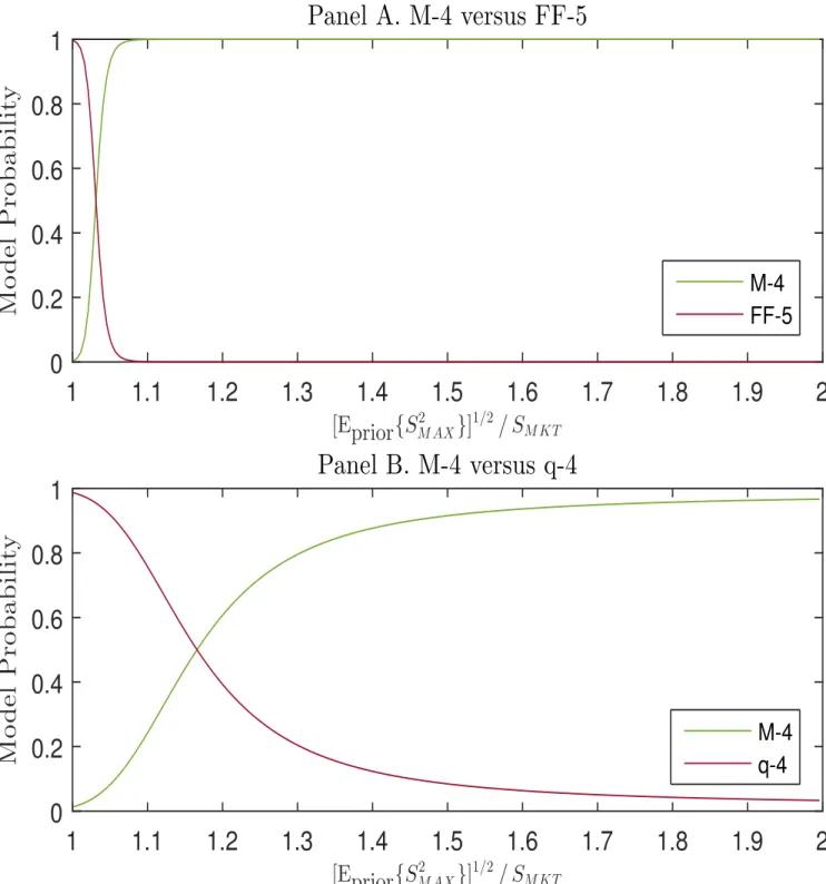
a Sharpe ratio can be produced by combining a given set of assets, in this case the assets represented by the model’s factors. Specifically, the prior implies a value for the expected maximum squared Sharpe ratio, relative to the (observed) Sharpe ratio of the market. We use the Barillas and Shanken (2015a) analytical results here to compute posterior model probabilities in the above two-way model comparison. Prior model probabilities of each model are set to one-half.21
Panel A of Figure 1 displays posterior probabilities in a comparison of model M-4 to model FF-5. The value on the horizontal axis is the square root of the prior expected maxi-mum squared Sharpe ratio achievable by combining the model’s factors, [Eprior{S2
M AX}]
1/2
, divided by the observed Sharpe ratio of the market, SM KT. We see in Panel A that when
21
We do not simultaneously compare three or more models, because assigning prior probabilities to models with differing degrees of similarity becomes more complicated. For example, assigning prior probabilities of 1/3 to each of models FF-5, q-4, and M-4 seems unreasonable, in that FF-5 and q-4 are more similar to each other than to M-4, as both FF-5 and q-4 include profitability and investment factors. For a category-based approach to such a problem, see Barillas and Shanken (2015a).
this Sharpe-ratio multiplier is only 1.01 or so, corresponding to a prior expectation that the market’s Sharpe ratio can be improved only very modestly, the data favor FF-5. The model probabilities are about equal for a multiplier of 1.05, and then the probability of M-4 rises steeply for higher values, to nearly 1.0 for multipliers of 1.1 or higher. In other words, when the prior admits more than very modest improvement over the market’s Sharpe ratio, the data strongly favor M-4 over FF-5.
The posterior probabilities in the comparison of models M-4 and q-4 are reported in Panel B of Figure 1. Here again we see that for smaller values of the Sharpe-ratio multiplier, model M-4 is less favored than the alternative. The probabilities cross at a multiplier between 1.1 and 1.2, and then the probability of M-4 increases to near 1.0 as the multiplier increases to 2.0 or more. In this Bayesian comparison, as in the earlier comparisons, model q-4 again fares better than model FF-5 when compared to model M-4, but the latter is strongly favored to either alternative model if prior beliefs admit a reasonable chance of achieving a substantially higher Sharpe ratio than that of the market index.
The reason that the other models are favored over M-4 when the Sharpe-ratio multiplier is low is essentially that the maximum Sharpe ratio produced by the M-4 factors is higher than for the other models. The Sharpe ratio of the market in our sample period is 0.11, and a multiplier of, say, 1.2 corresponds to an expected maximum Sharpe ratio of roughly just 0.13. In contrast, the sample produces a maximum Sharpe ratio for the M-4 factors equal to 0.49, higher than the maximum Sharpe ratios of 0.35 and 0.45 produced by the FF-5 and q-4 factors, respectively. Given that the sample maximum Sharpe ratio for M-4 is in greatest conflict with a value on the order of 0.13, that model receives the lowest posterior probability when the prior favors such a low maximum Sharpe ratio.
3.4.
Robustness
As discussed earlier, a number of the methodological choices we make when constructing our factors deviate somewhat from conventions that originate with Fama and French (1993) and are adopted in later studies such as Fama and French (2015) and Hou, Xue, and Zhang (2015a). None of these choices are crucial to our model’s relative performance in explaining anomalies and the other models’ factors. For example, because we believe that the extremes of our mispricing measure best identify mispricing, we use breakpoints of 20% and 80% rather than the conventional 30% and 70%. If we recompute Tables 5, 6, and 7 using 30% and 70%, however, our conclusions remain unchanged. Model M-4 maintains its edge over
model q-4 and continues to outperform model FF-5 by a substantial margin. The same holds true if we apply the 20% and 80% breakpoints to just the NYSE universe, instead of to the NYSE/AMEX/NASDAQ universe that covers a broader range of the mispricing scores. The results in Tables 5, 6, and 7 are also not affected much by replacing our SMB, which uses only stocks in the middle category of the mispricing-score rankings, with the more standard version that averages returns across all three categories. If we make all of the above changes simultaneously, again the model comparisons do not change materially. The online appendix reports all of these results.
In cases where annual data are used to construct factors in model FF-3 of Fama and French (1993), model FF-5 of Fama and French (2015), and model q-4 of Hou, Xue, and Zhang (2015a), the authors of those studies require a gap after the end of the fiscal year of at least 6 months and potentially up to 18 months. When using annual data, we instead require a gap of at least 4 months, following precedent in the accounting literature (e.g., Hirshleifer, Hou, Teoh, and Zhang (2004)). Thus, one potential source of performance differ-ences between our model, M-4, and models FF-5 and q-4 is this difference in timing used to contruct factors. To explore this possibility, we reconstruct the factors SMB and HML in model FF-3, SMB, HML, RMW, and CMA in model FF-5, and I/A in model q-4, which rely on annual data, by imposing the minimum gap of 4 months for information from annual statements, while using immediate prior-month values of market capitalization. Again our key results—Tables 5, 6, and 7—are not very sensitive to modifying models FF-5 and q-4 in that fashion. The online appendix reports these results as well.
We also investigate the stability of our results by splitting our overall 47-year period into two subperiods: 1967–1990 (24 years) and 1991–2013 (23 years). First, each of the 11 anomalies we use to construct the factors produces positive long-short FF-3 alphas in both subperiods. In the earlier subperiod, the t-statistics for the long-short alphas range from 1.5 to 5.4 across the 11 anomalies and average 3.4. In the later subperiod, the t-statistics range from 1.2 to 5.0 and again average 3.4. Second, in each subperiod, the assignment of anomalies to the two clusters is identical to that of the overall period, using either of the two methods described earlier. Finally, the superiority of model M-4, as indicated by the results in Tables 5 and 7, is supported consistently across both subperiods. The online appendix reports the results of these model comparisons in each subperiod.
3.5.
Factors and Return Variance
Factor models are generally viewed as useful not just for explaining expected returns. An additional role of factor models is to capture systematic time-series variation in realized returns. We briefly explore the extent to which mispricing factors can perform this role as compared to the factors in the alternative models we consider. For various sets of assets, we compute the R-squared in a regression of each asset’s monthly return on the factors for a given model. We then average those R-squared values across the assets.
Table 8 reports the average R-squared values obtained for five different sets of assets: 30 industry portfolios plus four sets of 25 portfolios formed with independent two-way 5×5 sorts of stocks on size and either book-to-market (B/M); the 11-anomaly composite mispricing measure used by Stambaugh, Yu, and Yuan (2015) (and used below to form the factor in model M-3); market beta; and return volatility.22
We estimate the regressions for six factor models: one with just the excess market return (MKT); one withMKT plus the size-factor (SMB) from the factor model (FF-3) of Fama and French (1993); the latter three-factor model; the five-three-factor model (FF-5) of Fama and French (2015); the four-three-factor model (q-4) of Hou, Xue, and Zhang (2015a); and model M-4. The factor betas on the assets are treated as constant over the sample period, so we probably understate the fraction of variance a given set of factors could explain if the betas were modeled as time-varying. Such a generalization lies beyond our study. We suggest the simple exercise reported briefly here nevertheless provides some insight into the relative abilities of the factor models to capture return variance.
We see in the first row of Table 8 that the market factor on average explains 59.5% of the variance of monthly industry returns. Adding a size factor increases that average R-squared only slightly, to 61.1%, and the other factor models further increase the R-squared only modestly. Model M-4 explains 63.3%, very close to the values of 63.6% for model q-4 and 63.5% for model FF-3. Thus, the model that does best in explaining anomalies—model M-4—does not appear to do so by sacrificing much if any ability to capture variance of industry returns.
For the remaining four sets of assets, the most salient difference from the industry results is that the size factor improves the R-squared substantially over that obtained with just a single market factor. This outcome is not surprising, as size is one of the sorting variables
22
We thank Ken French for providing on his website the returns for the 30 industry portfolios as well as the size-B/M, size-beta, and size-volatility portfolios.
used to form these sets of portfolios. Including the size factor adds roughly 8% to 10% to the R-squared produced by just the market factor. The further increases produced by including the additional factors in the other factor models are generally more modest, and the relative ranking of the R-squared values depends on which sorting variable is used in addition to si