Qing, Chunmei and Ruan, Jiawei and Xu, Xiangmin and Ren, Jinchang
and Zabalza, Jaime (2018) Spatial-spectral classification of hyperspectral
images : a deep learning framework with Markov random fields based
modeling. IET Image Processing. pp. 1-12. ISSN 1751-9659 ,
http://dx.doi.org/10.1049/iet-ipr.2018.5727
This version is available at
https://strathprints.strath.ac.uk/65510/
Strathprints is designed to allow users to access the research output of the University of Strathclyde. Unless otherwise explicitly stated on the manuscript, Copyright © and Moral Rights for the papers on this site are retained by the individual authors and/or other copyright owners. Please check the manuscript for details of any other licences that may have been applied. You may not engage in further distribution of the material for any profitmaking activities or any commercial gain. You may freely distribute both the url (https://strathprints.strath.ac.uk/) and the content of this paper for research or private study, educational, or not-for-profit purposes without prior permission or charge.
Any correspondence concerning this service should be sent to the Strathprints administrator:
The Strathprints institutional repository (https://strathprints.strath.ac.uk) is a digital archive of University of Strathclyde research outputs. It has been developed to disseminate open access research outputs, expose data about those outputs, and enable the
1
Spatial-Spectral Classification of Hyperspectral Images: A Deep Learning
Framework with Markov Random Fields Based Modeling
Chunmei Qing
1, Jiawei Ruan
1, Xiangmin Xu
1*, Jinchang Ren
2, Jaime Zabalza
2 1School of Electronic and Information Engineering, South China University of Technology, Guangzhou, China 2
Department of Electronic and Electrical Engineering, University of Strathclyde, Glasgow, United Kingdom *
Abstract: For spatial-spectral classification of hyperspectral images (HSI), a deep learning framework is proposed in this paper, which consists of convolutional neural networks (CNN) and Markov random fields (MRF). Firstly, a CNN model to learn the deep spectral feature from the HSI is built and the class posterior probability distribution is estimated. The CNN with a dropout layer can relieve the overfitting in classification. The CNN is utilized as a pixel-classifier, so it only works in the spectral domain. Then, the spatial information will be encoded by MRF-based multilevel logistic (MLL) prior for regularizing the classification. To derive the correlation of both spectral and spatial features for improving algorithm performance, the marginal probability distribution in HSI is learned using MRF-based loopy belief propagation (LBP). In comparison with several state-of-the-art approaches for data classification on 3 publicly available HSI datasets, experimental results have demonstrated the superior performance of the proposed methodology.
Keywords Hyperspectral image (HSI); spatial-spectral classification; convolutional neural networks (CNN); Markov random fields (MRF); loopy belief propagation (LBP).
1. Introduction
Hyperspectral remote sensing, a technology of acquiring remote sensing image in high-resolution spectrum, is capable of simultaneously collecting spectral and spatial information for earth observation, especially land cover analysis [1]. As an emerging field, hyperspectral remote sensing has been introduced in a wide range of scenes increasingly. Even for hyperspectral image (HSI)-based classification and target detection, the technology has been successfully applied in aerospace, agriculture, forestry, mineral, atmospheric sciences, military and so on [2][3]. Apart from these conventional applications, HSI also has great potential in health and pharmaceutical areas for its nature of non-intrusive inspection [4][5].
Due to the 3D hypercube it contains, image classification with HSI is always challenging [6]. The first reason is from the large volume and 3D data structure, where a high degree of redundancy in both spectral and spatial domain can be found. Another key drawback is the lack of sufficient training samples. Other issues may affect the classification include the spectral mixture, noise and so on. As a result, it is not straightforward to apply conventional machine learning approaches for HSI classification.
The support vector machine (SVM), capable of dealing with dataset in high-dimensional feature spaces, is found suitable for HSI classification [7], especially under a limited number of training samples for learning [8]. As an alternative, a multinomial logistic regression (MLR) [9] model, represented as modelling the conditional probability directly, doesn‟t need to care about joint probability distribution in dataset, yielding a good performance in hyperspectral image classification. For dealing with the high-dimensional classifications, sparse
representation-based classifier (SRC) is another useful solution [10]. Based on learning an over-complete dictionary, the high-dimensional data can be represented as a sparse expression which contains a large amount of zero coefficients, and hence it is discriminative to make a significant classification [11][12].
Recently, lots of novel methods about feature extraction and dimensionality reduction are employed in HSI data, for pre-processing the contiguous spectral bands with high redundancy in HSI [13]. Through preserving the discriminative features in low-dimensional space, it leads to a significant performance in HSI classification. In experiments, the traditional classifiers, generally which is SVM classifier, combined with some feature extraction methods, such as PCA, can obviously outperform previous methods [14]-[17].
The approaches mentioned above merely consider the spectral classification. However, the spatial information is also significant for spatial-spectral processing of HSI [18]. For example, the Morphological Profiles of HSI are important features for spectral-spatial classification, thus a number of methods about utilizing Morphological attribute Profiles or extended morphological profile (EMP) in classification of HSI are carried out in recent years [19]-[21].
Among many other approaches such as morphological filtering [22], maximum noise fraction (MNF) [23] and Nonnegative Matrix Factorization (NMF) [24], Markov random fields (MRF) is particularly useful as it helps to extract the spatial dependency in a Bayesian method for HSI classification. In [6], a novel MRF-based MLR classifier is proposed. And a SVM-MRF method for spectral-spatial classification is introduced in [25], where spatial information is used for refining the pixelwise classification from SVM.
2 In recent years, deep learning has been widely used
in many applications such as image processing, natural language understanding, speech recognition and artificial intelligence [26]. Recently, in the field of remote sensing image analysis, classification and target detection, deep learning has also been introduced [27]-[30], because of its powerful capacity of unsupervised deep features self-learning. Ref. [31] introduced the Convolutional Neural Networks (CNN) for HSI classification based on pixel vector, i.e., only using the spectral features. Later, 2D-oriented CNN in [32] encoded the spectrum by PCA and classified each pixel with its spatial neighbouring pixels as 2D input. On this basis, 3D-CNN can reserve the whole spectral bands [33], which sufficiently exploit both the spectral and spatial features through a large-scale network. However, as the network being more complex and high-dimensional, it takes longer runtime for computation. Stacked Auto-Encoders (SAE) also can perform well in the spectral-spatial classification [34]. More CNN-based methods are explored in [40] [41]. Furthermore, Ref. [42] proposed the Mugnet using limited samples. Ref. [43] used RNN for hyperspectral image processing. Ref. [44] proposed a deep feature fusion network. Semi-supervised network using pseudo labels was presented in [45]. Gabor filtering based deep network was proposed in [46]. And residual network is utilized in [47].
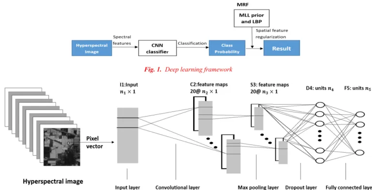
In this paper, a deep learning framework with MRF-based model is proposed for spectral-spatial classification of HSI. As shown in Fig. 1, this framework consists two key parts: CNN classifier and MRF, which are used for spectral classification and spatial regularization, respectively. The characteristics of the proposed approach can be highlighted as follows.
1) A deep CNN model is built to learn the deep features and the classification of HSI. In this step, the input of the CNN is the pixel vectors in HSI containing the spectrum, so the CNN will be a pixel-classifier.
2) Markov random field is employed to utilize the spatial information. The MRF-based multilevel logistic (MLL) prior, which forces a
smooth segmentation,
encodes the spatial information to regularize the classification result obtained in CNN. In addition, to derive the correlation of both spectral and spatial features for improved algorithm performance, MRF-based loopy belief propagation (LBP) is adopted to learn the marginal probability distribution in HSI.3) Compared with the traditional 3D-CNN model, the propose method not only can learn the deep features from HSI itself, but also can save large amount of computation because of its simple structure for feature learning in pixel level. Furthermore, spectral-spatial information from all pixels of HSI in MRF is utilized, while the 3D-CNN merely takes advantage from neighbouring pixels. Extensive experiments demonstrate the outperforming performance of the proposed CNN-MRF approach.
The remainder of this paper is organized as follows. Section 2 formulates proposed deep learning framework. Section 3 demonstrates the experimental results in benchmarking with state-of-the-art approaches. Finally, Section 4 summarizes the conclusions.
2. Proposed Deep Learning Framework Based on MRF
2.1. Convolutional neural networks for classification
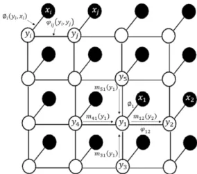
In the proposed deep learning framework, CNN is employed to extract deep features and make classification result. As shown in Fig. 2, the network structure of the proposed CNN can be divided into five layers, including an input layer, a convolutional layer, a max pooling layer, a dropout layer and a fully connected layer [31]. Therefore, it Fig. 1. Deep learning framework
3 is a simple CNN, with only one hidden layer, means the
model‟s depth is one.
Generally, the input of CNN is a 2D image. In fact, hyperspectral image classification is to consider each pixel as an input signal. For the HSI, a pixel represents the reflection in all bands on a geospatial point, shown as a continuous spectrum. In our proposed method, each HSI pixel can be regarded as 2D image whose length is n (n denotes the number of channels) and height is equal to 1, thus each pixel can be as the input of the CNN. Assume that the number of pixels is in HIS. Let
denotes the image of n-dimensional feature vectors.
For each pixel every is
assigned to a label , so let represents the output, i.e., label image for the input image, where
denotes a set of C classes.
Input layer I1 stores the pixel vector, with a size of where is the number of HSI bands. Convolutional layer C2 uses 20 kernels with the size of to convolution. The step between the local receptive fields is 1. Thus, layer C2 outputs 20 feature maps
of size and . Since every filter
has weights and 1 bias, there are trainable parameters in layer C2. The max pooling layer S3, with the kernel size of , outputs 20 feature maps of size , where . There is no parameter in our max pooling layer. The dropout layer D4, outputs units and there are trainable parameters in layer D4. Architecturally, the dropout layer has a same structure as fully connected layer, but it works differently in the training process, which we will introduce later. The fully connected layer F5, which is also the output layer, outputs units, where denotes the number of classes. There are trainable parameters in layer F5.
In the proposed structure, layer C2 and layer S3 can be viewed as the feature extraction of the input data, while layer D4 and layer F5 make up a classifier of the features. As [35] recommended, the weighs set is in the
interval , where denotes the units‟
number outputted from previous layer, and all the bias vector set as 0.
The training process consists 2 iterative steps: forward propagation and back propagation, which are mentioned as follows.
1) Forward propagation
Forward propagation is aimed at obtain the classification result of the input according to the current parameters.
Assuming is the input data of i-th layer, then its output data is also the input data for the next layer, denoted as . The expression of each layer can be written as
(1) where
, (2) and is an activation function, denotes weight matrix and denotes bias vector. Since the sparseness of linear model is not strong enough, the activation function is recommended as non-linear model.
Specifically, hyperbolic tangent function is chosen in the convolutional layer . Lots of experiments have proved it has the best performance[30]. The maximum function is used in pooling layer
, so it also called max pooling layer. The layer D4 still choose the hyperbolic tangent function
. Since it is a multiclass classification, softmax function is adopted in output layer F5:
The final output denotes the classification result with the current parameters in CNN. Obviously, the densities is determined by the CNN.
2) Back propagation
Back propagation is employed to update the parameters of CNN for minimizing the error between the training model output and the desired classification result. We employ the gradient descent method to update network parameters in the back propagation stage.
Since the output layer F5 adopts softmax function as its activation function, for softmax regression model, the error is given by
(3) where denotes the number of training samples,
denotes output units in output layer which is equaled to the number of class, and are the desired target output and the current output response to the m-th input data, respectively, and is the c-th element of the . If the sample belongs to class c, the k-th element of is positive and the rest of will be zero. is an indicator function and means, if c is equal to , the value of the desired output of m-th sample is 1, otherwise its value is 0. A minus sign added to the front of the equation can make the computation more convenient.
For the other layer hyperbolic tangent function is chosen as their activation function, we consider error by the squared-error loss function
(4) where is the number of output units.
The error propagate backwards through the network can be viewed as the “sensitivities” of each unit. Here, we compute derivatives of E with respect to as its sensitivities in i-th layer. It is given by
(5) where ° denotes element-wise multiplication. And the sensitivities of output layer is given by
. (6) It can be obtained by calculated that
(7) As , we have , (8) . (9) Then the trainable parameters are updated by
4 (11)
where is the learning rate.
With the increase of the number of iteration, the output of CNN will be increasingly closer to the desired label output. Specially, we should pay more attention to the back propagation in convolutional layer. Because of sub-sampling, the number of sensitivities in pooling layer is not match the convolutional layer so that it cannot implement (5) directly. Actually, each unit in pooling layer corresponds to a block of units in convolutional layer‟s output maps.
Therefore, for calculating the sensitivities in convolutional layer, we should up-sample the sensitivity maps in pooling layer to make it as large as the one in convolutional layer, which means just multiply the activation derivative at current layer element-wise
(12) where denotes an up-sampling operation. A simple method is to copy the sensitivity maps times, where is the sampling factor in pooling layer.
Finally, the gradients for the bias is equal to the sensitivities as (9) implemented. But in consideration of the convolutional layer having same sharing weights, if calculate the gradient for a given weight, we just need to multiply a patch of the input connected to the weight with the corresponding sensitivities
(13) where denotes a parameter of the weights matrix , denotes the patch of input connected to the weight , and
denotes the sensitivity map corresponded to the in the position .The parameter update is still implemented as (10) and (11).
3) Dropout
Adding dropout layer in CNN is useful to relieve the overfitting by preventing the complex co-adaptations in training processing [36]. As we mentioned above, the dropout layer has a same structure as fully connected layer, but it works differently in the training process. In fact, it can be view that dropout layer is the fully connected layer using “dropout”.
As shown in Fig. 3, in each training iteration, the units in dropout layer will randomly “dropout”. The dropout probability is set to 0.5 as recommended in [36]. It makes some weights in the network sometimes not work but still exists. It can be seen that we have trained lots of different network like Fig. 3(b), and obtain an ensemble learning
network at last.
After the training process, we need to multiply the dropout rate (0.5) with the weights in dropout layer in order to keep the magnitudes have no change.
2.2. MRF-based MLL prior for spatial features regularization
Given the input , the trained CNN can extract the deep features from spectral features and make classification result. It means that CNN models the densities . However it means only spectral information is considered in classification, while spatial information is wasted. Therefore, the spatial information is incorporated by using multilevel logistic prior, which belongs to the Markov Random Fields.
In the Bayesian approach, classification results is generally given by maximizing the posterior distribution [6]. The maximum a posterior (MAP) estimates the class result, which means that given input X, it estimates result y when maximizing . Under Bayes‟ theorem, MAP estimate can be written as
(14) where denotes the prior over the labels in y, and is a likelihood function which means the probability of input data given the labels.
Assuming in conditional independence
(15) can be written as (16)
where is a coefficient without
dependency to y. The MAP classification is finally implemented as
(17)
The proposed method will adopt the MAP classification as the final classification result. In (17), the density given by the pixel-classifier modeled by CNN with spectral features, while the MRF-based MLL
(a) (b)
Fig. 3. (a) Full connection in training. (b) Dropout in training
5 prior will be used as the prior to encode the spatial
information. To solve this problem, MRF-based loopy belief propagation (LBP) algorithm is used, which can also learn the correlation of both spectral and spatial features.
According to the Hammersley-Clifford Theorem, the Gibbs‟ distribution expresses the probability of the relevance in MRF [6]. So the MLL prior is given by
(18)
where denotes the normalizing constant, is the parameter controlling the smoothness, denotes a set which consists of pair of neighbouring pixels, and is a unit
impulse function, where and .
The MLL prior encourages that it is with a high probability for the neighbouring pixels having a same label, and hence it promotes piecewise smooth classification. Combined (17) with (18), the MAP estimation is finally given by
(19) Minimization of the equation in (19) refers to a complex combinatorial optimization problem, and thus LBP algorithm is put forward to solve this problem [18].
2.3. Loopy belief propagation for learning marginal probability
As Fig. 4 shown, in the MRF‟s model, the hidden nodes and the observed nodes appear pairwise, i.e., each label is related to an respective input . LBP algorithm can not only solve the problem in (19) but also learn the marginal probability for each label [37].
The classification in this model amounts to infer the hidden information via observe the information . Each node has a hidden nodes and an observed nodes . In the square lattice, denotes the statistical relation between input and label , and , which is learned by CNN in above. represents the interaction potential, which reflects the continuity of the neighbouring labels, i.e., penalizes dissimilar pair of neighbouring labels. Thus the MLL prior is proposed to urge a smooth label image.
LBP is an iterative algorithm that propagates message through the nodes to update the state of MRF constantly until being convergence [37]. In each iteration, the spectral message and spatial message are propagated to the neighbour and go on in next iteration. Finally, LBP will learn the marginal probability which contains both the spectral and spatial probability. As shown in Fig. 4, the message sent from label to its neighboring label is defined as
(20)
where denotes the normalization constant, and denotes all the neighboring labels of label except the label .
In each iteration, all the labels send message to and receive message from their neighbours, as shown in Fig. 5. The belief in each label is given by all the incoming messages, therefore, the belief of label , i.e., the marginal probability is estimated by the joint probability distribution
(21)
where denotes all the neighboring labels of label . The details of LBP algorithm is given in Algorithm LBP. The details of the proposed framework are summarized in Algorithm HSI.
Algorithm LBP
1:Initialize all the labels‟ belief 2:For iter = 1 to Training iteration do
Select a pair of neighbouring labels randomly; Label propagate message to label , (20); Update the belief of label , i.e., , (21); End
3:Compute the posterior probability :
(22)
Algorithm HSI
CNN training
1:Initalize all the parameters as proposed 2:Constract the CNN model as shown in Fig. 2 3:Generate weights W and bias b
4:While err < MinError do For batch = 1 to Batches do y = FP(TrainingData), (1)(2);
[E, ] = BP(TrainingLabel), (3)(5)(6); Update W, b using (10)(11);
err = err + mean(E); End err = err/Batches End CNN classification 1: = FP(TestingData) MRF-based MLL prior 1: = MLL(ImageSize) LBP
1:Initialize all the labels‟ belief
2:For iteration = 1 to Training iteration do
Select a pair of neighboring labels randomly; Label propagate message to label , (22); Update the belief of label , i.e., , (21); End
3:Compute the posterior probability :
Fig. 5. The message propagates in LBP
6
3. Experimental Results
3.1. Hyperspectral data sets description
To validate the feasibility of proposed deep learning framework and test its performance, 3 different publicly available remote sensing datasets are used in the experiments.
1) Indian Pines data set
The first hyperspectral dataset is gathered by AVIRIS sensor over Indian Pines test site in North-western Indiana, and consists of 145x145 pixels with a spatial resolution of 20m per pixel, and 224 spectral bands in the wavelength range from 0.4 to 2.5 . Due to the noise and water absorption phenomena, bands covering the region of water absorption ([104-108], [150-163], 220) are abandoned, leaving 200 channels employed in experiments. This dataset has a size of 145x145x200. The ground truth map of Indian Pines HSI is shown in Fig. 6(a), which contains 10249 labeled pixels belongs to 16 classes. The training set will randomly select almost 10% from the dataset, and the remaining data makes up the testing set. The training set‟s samples in each class is quite unbalanced. Table I lists the details of the number of pixels and classes.
2) Pavia University data set
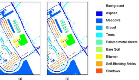
The second hyperspectral dataset is acquired by ROSIS optical sensor over University of Pavia, Italy, and consists of 610x340 pixels with a spatial resolution of 1.3m per pixel. This image comprises 103 spectral channels and a data size of 610x340x103. The ground truth map of Pavia University HSI is shown in Fig 7(a), which contains 42776
labelled pixels belongs to 9 classes. The training set will randomly select 200 pixels per class from the dataset, and the remaining data makes up the testing set. Table II lists the details of the number of pixels and classes.
3) Salinas Scene data set
The third hyperspectral dataset is gathered by 224-band AVIRIS sensor over Salinas Valley, California, and consists of 512x1217 pixels with high spatial resolution of 3.7m per pixel. Similarly to the Indian Pines scene, 20 water absorption bands ([108-112], [154-167], 224) are removed, leaving 204 bands used in experiments. This dataset has a size of 512x217x204. The ground truth image of Salinas Scene HSI is shown in Fig 8(a), which contains 52322
TABLEI
CLASSES AND NUMBERS OF PIXELS ON THE INDIAN PINES DATASET
Class Samples
No. Name Train Test
1 Alfalfa 10 36 2 Corn-no till 143 1285 3 Corn-min till 83 747 4 Corn 24 213 5 Grass-pasture 48 435 6 Grass-trees 73 657 7 Grass-pasture-mowed 10 18 8 Hay-windrowed 48 430 9 Oats 10 10 10 Soybean-no till 97 875 11 Soybean-min till 246 2209 12 Soybean-clean 59 534 13 Wheat 21 184 14 Woods 127 1138 15 Bldg-Grass-Trees-Drives 39 347 16 Stone-Steel-Towers 10 83 Total 1048 9201 TABLEII
CLASSES AND NUMBERS OF PIXELS ON THE PAVIA UNIVERSITY DATASET
Class Samples
No. Name Train Test
1 Asphalt 200 6431 2 Meadows 200 18449 3 Gravel 200 1899 4 Trees 200 2864 5 Metal sheets 200 1145 6 Bare soil 200 4829 7 Bitumen 200 1130 8 Bricks 200 3482 9 Shadows 200 747 Total 1800 40976 TABLEIII
CLASSES AND NUMBERS OF PIXELS ON THE SALINAS SCENE DATASET
Class Samples
No. Name Train Test
1 Brocoli_green_weeds_1 20 1989 2 Brocoli_green_weeds_2 37 3689 3 Fallow 20 1956 4 Fallow_rough_plow 14 1380 5 Fallow_smooth 27 2651 6 Stubble 40 3919 7 Celery 36 3543 8 Grapes_untrained 113 11158 9 Soil_vinyard_develop 62 6141 10 Corn_senesced_green_weeds 33 3245 11 Lettuce_romaine_4wk 11 1057 12 Lettuce_romaine_5wk 19 1908 13 Lettuce_romaine_6wk 9 907 14 Lettuce_romaine_7wk 11 1059 15 Vinyard_untrained 73 7195 16 Vinyard_vertical_trellis 18 1789 Total 543 51779
7 labelled pixels belongs to 16 classes. The training set will
randomly select almost 1% from the dataset, and the remaining data makes up the testing set. The training set‟s samples are quite small. Details of the number of pixels and classes are listed in Table III.
3.2. Configuration for CNN
Since the three data sets have different spectral channels, it needs to set different parameters for them. As recommended in [22], is better to be , and . can be any number between 30 and 40, and . is better to be set to 100. These choices might not be the best but are effective for general HSI data. Therefore, for the Indian Pines dataset with 200 bands (after preprocessing) in 16 classes, we set the layer parameters of
CNN: , , , , ,
, . For the Pavia University dataset with 103 bands in 9 classes, we set the layer parameters of CNN:
, , , , , ,
. For the Salinas Sense dataset with 204 bands in 16 classes, we set the layer parameters of CNN: ,
, , , , ,
The learning rate is set to 0.03. The effect of several parameters will be discussed later.
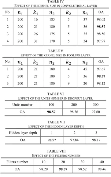
The classification performance is illustrated by overall accuracy (OA), average accuracy (AA) and Kappa statistic. To validate whether those proposed configuration for our CNN is appropriate, we analyse the effect of the layer parameters, layer depth, units of dropout layer and filter numbers here. The control variable method is employed in this experiment, where the Indian Pines dataset is used.
From the experimental results shown in Table IV, among different kernel size of convolutional layer (16, 21, 26 and 31), the better accuracy is obtained when the is closer to be , i.e. , when the other parameters is unchanged. Then we discuss the size of the pooling layer . As shown in Table V, when
and is between 30 and 40, the useful information is kept furthest.
Similarly, it can be seen that higher hidden layer depth (2 and 3) or number of units in dropout layer (200 and 300) is not necessarily to improve the classification performance, as Table VI and Table VII show. In fact, a low depth or a few number of units may give rise to under-fitting, but the proposed network is enough satisfied with solving this problem. Under the limited number of training samples, more complex networks may be faced with overfitting. In addition, a simple CNN with low layer depth can reach a fast speed in training iterations, which will save more training time.
The number of filters is shown in Table VIII. It can be seen that 20 filters is adequate to extract the required deep features in our framework.
3.3. Experiments with Indian Pines dataset
State-of-the-art methods for HSI classification will be applied in the experiments as comparison, which include:
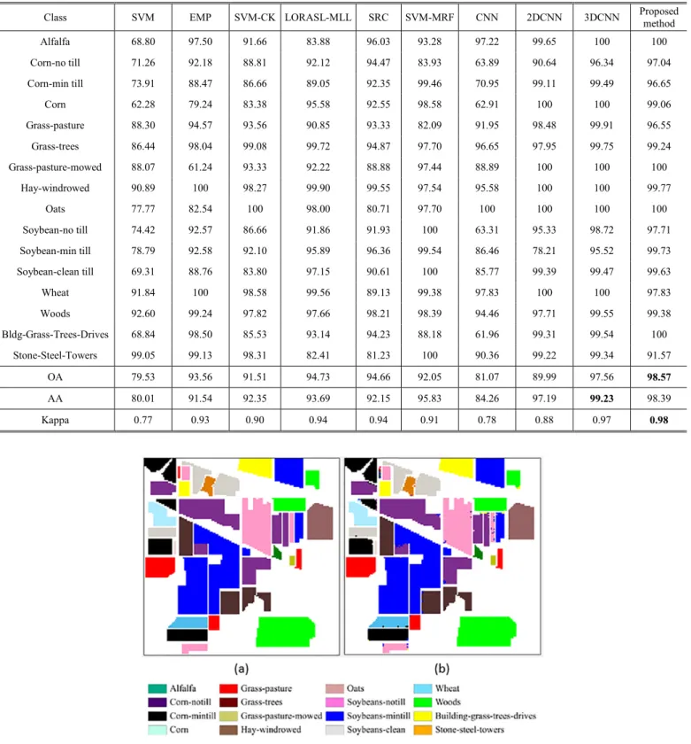
SVM [8], EMP [21], SVM-composite kernel (SVM-CK) [38], LORSL-MLL [6], sparse representation-based classification (SRC) [10], SVM-MRF [25], CNN [31], 2DCNN [32] and 3DCNN [33], [39]. The SVM only considers the spectral information, implemented by the Gaussian kernel. On this basic, the spatial information is exploited by the EMP, composite kernel and MRF respectively for EMP [21], SVM-CK [38] and SVM-MRF [25]. LORSL-MLL is a classical method with MLL prior. As mention above, the CNN, 2DCNN and 3DCNN are the deep learning method but deal with the HSI classification in different dimensional of input data.
Table IX illustrates the experimental results by different classification algorithms with the Indian Pines data set. From the experimental results, the SVM and the CNN classifier, which only consider the spectral features, obtain bad classification results. While taking advantage of the spatial information, the other methods have a superior performance. What‟s more, the 3DCNN and the proposed method, which extract the deep features from the original data, achieve higher accuracy. Compared to the 3DCNN, the experimental results illustrate the better performance of the proposed deep learning framework, because the 3DCNN merely takes advantage from neighboring pixels, while the proposed method exploits spectral-spatial information from all pixels of HSI in MRF.
TABLEV
EFFECT OF THE KERNEL SIZE IN POOLING LAYER
No. OA
1 200 21 180 4 45 97.67
2 200 21 180 5 36 98.57
3 200 21 180 9 20 98.12
TABLEVII
EFFECT OF THE HIDDEN LAYER DEPTH
Hidden layer depth 1 2 3
OA 98.57 97.84 98.17
TABLEVI
EFFECT OF THE UNITS NUMBER IN DROPOUT LAYER
Units number 100 200 300
OA 98.57 98.36 97.60
TABLEVIII EFFECT OF THE FILTERS NUMBER
Filters number 10 20 30 40
OA 98.20 98.57 98.52 98.46
TABLEIV
EFFECT OF THE KERNEL SIZE IN CONVOLUTIONAL LAYER
No. OA
1 200 16 185 5 37 98.02
2 200 21 180 5 36 98.57
3 200 26 175 5 35 98.50
8 The superior performance of the proposed
CNN-MRF makes a strong contrast with the SVM-CNN-MRF and CNN. It can be seen that both the CNN and MRF play a key role in the framework, and none is dispensable. Fig. 6(b) shows the classification map.
3.4. Experiments with Pavia University dataset
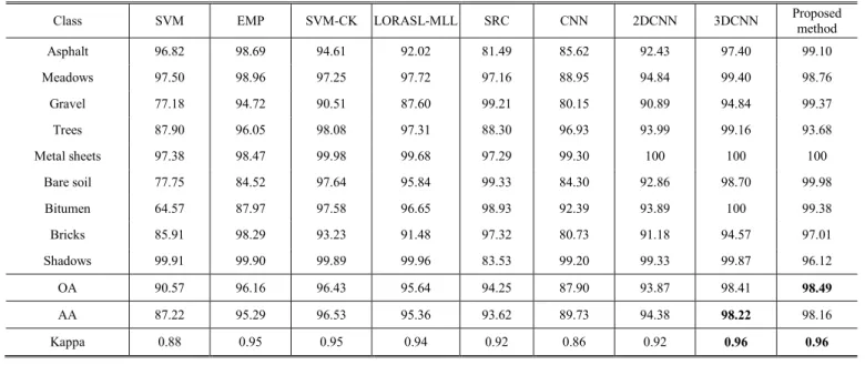
Table X reports the experimental results by different classification algorithms in the Pavia University data set, and the proposed method performs better than those
compared classification algorithms. Fig. 7(b) shows the classification map.
3.5. Experiments with Salinas Scene dataset
Table XI reports the experimental results by different classification algorithms in the Salinas Scene data set, and the proposed method performs better than those compared classification algorithms. Fig. 8(b) shows the classification map
TABLEIX
DIFFERENT CLASSIFICATION ALGORITHMS APPLIED TO THE INDIAN PINES DATASET
Class SVM EMP SVM-CK LORASL-MLL SRC SVM-MRF CNN 2DCNN 3DCNN Proposed
method Alfalfa 68.80 97.50 91.66 83.88 96.03 93.28 97.22 99.65 100 100 Corn-no till 71.26 92.18 88.81 92.12 94.47 83.93 63.89 90.64 96.34 97.04 Corn-min till 73.91 88.47 86.66 89.05 92.35 99.46 70.95 99.11 99.49 96.65 Corn 62.28 79.24 83.38 95.58 92.55 98.58 62.91 100 100 99.06 Grass-pasture 88.30 94.57 93.56 90.85 93.33 82.09 91.95 98.48 99.91 96.55 Grass-trees 86.44 98.04 99.08 99.72 94.87 97.70 96.65 97.95 99.75 99.24 Grass-pasture-mowed 88.07 61.24 93.33 92.22 88.88 97.44 88.89 100 100 100 Hay-windrowed 90.89 100 98.27 99.90 99.55 97.54 95.58 100 100 99.77 Oats 77.77 82.54 100 98.00 80.71 97.70 100 100 100 100 Soybean-no till 74.42 92.57 86.66 91.86 91.93 100 63.31 95.33 98.72 97.71 Soybean-min till 78.79 92.58 92.10 95.89 96.36 99.54 86.46 78.21 95.52 99.73 Soybean-clean till 69.31 88.76 83.80 97.15 90.61 100 85.77 99.39 99.47 99.63 Wheat 91.84 100 98.58 99.56 89.13 99.38 97.83 100 100 97.83 Woods 92.60 99.24 97.82 97.66 98.21 98.39 94.46 97.71 99.55 99.38 Bldg-Grass-Trees-Drives 68.84 98.50 85.53 93.14 94.23 88.18 61.96 99.31 99.54 100 Stone-Steel-Towers 99.05 99.13 98.31 82.41 81.23 100 90.36 99.22 99.34 91.57 OA 79.53 93.56 91.51 94.73 94.66 92.05 81.07 89.99 97.56 98.57 AA 80.01 91.54 92.35 93.69 92.15 95.83 84.26 97.19 99.23 98.39 Kappa 0.77 0.93 0.90 0.94 0.94 0.91 0.78 0.88 0.97 0.98
9
3.6. Effect of fewer number of training set
In last experiments, we attempt to reduce the number of training set to exam the proposed method in Indian Pines, Pavia University and Salinas Scene data sets: from 3% to 10% for Indian Pines, from 50 to 200 per class for Pavia University and from 0.4% to 1% for Salinas Scene.
Table XII, XIII and XIV illustrate the experimental results. It can be seen that classification accuracies increase
with the number of training set in accordance with expectation. The proposed method still achieves a superior performance when there are less training samples provided.
3.7 Processing Time
The experiments are implemented using MATLAB on a normally configured computer with Inter(R) Core(TM) i5-4460 CPU at 3.20 GHz and 8-GB RAM. The testing time of these experiments based on Table I, II, III are shown in Table XV. It should be noting that since the spatial
TABLEX
DIFFERENT CLASSIFICATION ALGORITHMS APPLIED TO THE PAVIA UNIVERSITY DATASET
Class SVM EMP SVM-CK LORASL-MLL SRC CNN 2DCNN 3DCNN Proposed
method Asphalt 96.82 98.69 94.61 92.02 81.49 85.62 92.43 97.40 99.10 Meadows 97.50 98.96 97.25 97.72 97.16 88.95 94.84 99.40 98.76 Gravel 77.18 94.72 90.51 87.60 99.21 80.15 90.89 94.84 99.37 Trees 87.90 96.05 98.08 97.31 88.30 96.93 93.99 99.16 93.68 Metal sheets 97.38 98.47 99.98 99.68 97.29 99.30 100 100 100 Bare soil 77.75 84.52 97.64 95.84 99.33 84.30 92.86 98.70 99.98 Bitumen 64.57 87.97 97.58 96.65 98.93 92.39 93.89 100 99.38 Bricks 85.91 98.29 93.23 91.48 97.32 80.73 91.18 94.57 97.01 Shadows 99.91 99.90 99.89 99.96 83.53 99.20 99.33 99.87 96.12 OA 90.57 96.16 96.43 95.64 94.25 87.90 93.87 98.41 98.49 AA 87.22 95.29 96.53 95.36 93.62 89.73 94.38 98.22 98.16 Kappa 0.88 0.95 0.95 0.94 0.92 0.86 0.92 0.96 0.96 TABLEXI
DIFFERENT CLASSIFICATION ALGORITHMS APPLIED TO THE SALINAS SCENE DATASET
Class SVM EMP SVM-CK LORASL-MLL SRC CNN 2DCNN 3DCNN Proposed
method Brocoli_green_weeds_1 99.74 99.84 91.66 99.44 100 98.73 98.84 100 99.55 Brocoli_green_weeds_2 99.01 99.76 88.81 99.95 99.98 99.12 99.61 99.89 99.84 Fallow 91.05 93.15 86.66 99.78 97.61 96.08 99.75 99.89 99.34 Fallow_rough_plow 97.04 98.49 83.38 98.34 83.24 99.71 98.79 99.25 97.68 Fallow_smooth 98.07 99.16 93.56 98.78 97.10 97.04 99.84 99.39 96.94 Stubble 99.98 99.98 99.08 99.83 97.63 99.59 99.70 100 99.77 Celery 98.89 99.92 93.33 99.66 99.57 99.33 79.05 99.82 99.58 Grapes_untrained 75.96 92.96 98.27 90.76 88.61 78.64 99.17 91.45 99.97 Soil_vinyard_develop 98.87 99.25 100 99.97 99.97 98.04 96.88 99.95 100 Corn_senesced _weeds 88.86 93.37 86.66 94.15 96.11 92.38 99.31 98.51 96.06 Lettuce_romaine_4wk 91.77 98.80 92.10 95.34 97.37 99.14 100 99.31 89.12 Lettuce_romaine_5wk 95.75 96.53 83.80 99.99 95.52 99.88 100 100 99.63 Lettuce_romaine_6wk 94.78 98.01 98.58 97.83 95.08 97.84 98.97 99.72 92.61 Lettuce_romaine_7wk 96.47 97.30 97.82 95.95 94.64 96.17 82.24 100 96.60 Vinyard_untrained 72.35 91.74 85.53 73.55 84.07 72.96 97.57 96.24 88.56 Vinyard_vertical_trellis 98.64 98.30 98.31 98.92 99.33 98.59 99.61 99.63 98.43 OA 89.33 96.23 91.51 93.75 93.96 90.25 92.39 97.42 97.44 AA 93.58 97.29 92.35 96.39 95.36 95.19 96.83 98.94 97.11 Kappa 0.88 0.95 0.90 0.93 0.93 0.90 0.92 0.97 0.97
10 information of all pixels is needed, the testing time is
proportional to the total number of pixels including both labelled and unlabelled pixels.
4. Conclusion
This paper mainly introduces a deep learning framework for spatial-spectral classification of HSI. The framework consists of two parts: CNN and MRF, respectively acting on classification with spectral features and regularization with spatial information. To derive the correlation of both spectral and spatial features for improving algorithm performance, the marginal probability distribution in HSI is learned using MRF-based loopy belief propagation (LBP). In the experiments, three widely used remote sensing datasets are utilized. Compared with several state-of-the-art approaches, the proposed framework achieves superior performance.
Although the proposed framework has satisfied performance, there are still some challenges, such as the parameter optimization, the cost of training time and so on. Therefore, our future work may focus on the parameters‟ adjustment and the computational time optimization.
Acknowledgments
This work is supported by the National Natural Science Foundation of China (Grant No. 61401163), the Science and Technology Planning Project of Guangdong
Province of China (No. 2014B010111003,
2014B010111006, 2016B010108008), and Guangzhou Key Lab of Body Data Science under Grant 201605030011.
References
[1] Lee, Z., Carder K.L.: „Hyperspectral Remote Sensing‟, Current Science, 2012, 94, pp. 1115-1116
[2] Cheng, G., Han, J., Lu, X.: „Remote Sensing Image Scene Classification: Benchmark and State of the Art‟, Proceedings of the IEEE, 2017, 99, pp. 1-19
[3] Cheng, G., Han, J.: „A Survey on Object Detection in Optical Remote Sensing Images‟, Isprs Journal of Photogrammetry & Remote Sensing, 2016, 117, pp. 11-28
[4] Noor, S., Michael, K., Marshall, S., et al.: „The properties of the cornea based on hyperspectral imaging: Fig. 7. (a) Ground truth map of Pavia University dataset. (b) Classification map acquired by proposed method for Pavia University dataset.
11 Optical biomedical engineering perspective‟. IEEE
International Conference on Systems, Signals and Image Processing., 2016, pp.1-4
[5] Fei, B., Akbari, H., Halig, L.V.: „Hyperspectral imaging and spectral-spatial classification for cancer detection‟. IEEE International Conference on Biomedical Engineering and Informatics., 2013, pp. 62-64
[6] Li, J., Bioucas-Dias, J.M., Plaza, A.: „A Spectral– Spatial Hyperspectral Image Segmentation Using Subspace Multinomial Logistic Regression and Markov Random Fields‟, IEEE Transactions on Geoscience & Remote Sensing, 2012, 50, pp. 809-823
[7] Fauvel, M., Benediktsson, J., Chanussot, J., Sveinsson, J.: „Spectral and spatial classification of hyperspectral data using SVMs and morphological profiles‟, IEEE Trans. Geosci. Remote Sens., 2008, 46, (11), pp. 3804- 3814
[8] Melgani, F., Bruzzone, L.: „Classification of hyperspectral remote sensing images with support vector machines‟, IEEE Transactions on Geoscience & Remote Sensing, 2004, 42, pp. 1779-1790
[9] Krishnapuram, B., Carin, L., Figueiredo, M., Hartemink, A.: „Sparse multinomial logistic regression: Fast algorithms and generalization bounds‟, IEEE Trans. Pattern Anal. Mach. Intell., 2005, 27, (6), pp. 957-968 [10]Chen, Y., Nasrabadi, N.M., Tran, T.D.: „Hyperspectral
image classification using dictionary-based sparse representation‟, IEEE Trans. Geosci. Remote Sens., 2011, 49, (10), pp. 3973-3985
[11]Du, P., Xue, Z., Li, J., Plaza, A.: „Learning Discriminative Sparse Representations for Hyperspectral Image Classification‟, IEEE Journal of Selected Topics in Signal Processing, 2015, 9, pp. 1089-1104
[12]Lu, X., Yuan, Y., Zheng, X.: „Joint Dictionary Learning for Multispectral Change Detection‟, IEEE Transactions on Cybernetics, 2017, 47, pp. 884-897
[13]Zheng, X., Yuan, Y., Lu, X.: „Dimensionality Reduction by Spatial-Spectral Preservation in Selected Bands‟, IEEE Transactions on Geoscience & Remote Sensing, 2017, 99, pp. 1-13
[14]Qiao, T., Yang, Z., et al.: „Joint bilateral filtering and spectral similarity-based sparse representation: A generic framework for effective feature extraction and data classification in hyperspectral imaging‟, Pattern Recognition, 2018, 77, pp. 316-328
[15]Zabalza, J., Ren, J., Zheng, J., et al.: „Novel Two-Dimensional Singular Spectrum Analysis for Effective Feature Extraction and Data Classification in Hyperspectral Imaging‟, IEEE Transactions on Geoscience & Remote Sensing, 2015, 53, pp. 1-16 [16]Zabalza, J., Ren, J., Yang, M., et al.: „Novel
Folded-PCA for improved feature extraction and data reduction with hyperspectral imaging and SAR in remote sensing‟, Isprs Journal of Photogrammetry & Remote Sensing, 2014, 93, pp. 112-122
[17]Ren, J., Zabalza, J., Marshall, S., et al.: „Effective feature extraction and data reduction with hyperspectral imaging in remote sensing‟, IEEE Signal Processing Magazine, 2014, 31, pp. 149-154
[18]Cao, F., Yang, Z.: „Sparse representation based augmented multinomial logistic extreme learning machine with weighted composite features for spectral-spatial classification of hyperspectral images‟, IEEE Transactions on Geoscience & Remote Sensing, 2018, pp. 1-17
[19]Li, J., Reddy Marpu, P., Plaza, A., et al.: „Generalized Composite Kernel Framework for Hyperspectral Image Classification‟, IEEE Transactions on Geoscience & Remote Sensing, 2013, 51, pp. 4816-4829
[20]Bao, R., Xia, J., Mura, M.D., et al.: „Combining Morphological Attribute Profiles via an Ensemble Method for Hyperspectral Image Classification‟, IEEE Geoscience & Remote Sensing Letters, 2016, 13, pp. 1-5
[21]Benediktsson, J.A., Palmason, J.A., Sveinsson, J.R.: „Classification of hyperspectral data from urban areas based on extended morphological profiles‟, IEEE Trans. Geosci. Remote Sens., 2005, 43, (3), pp. 480-491
TABLEXII
EFFECT OF FEWER NUMBER OF TRAINING SET (INDIAN PINES DATASET)
Percentage of Training samples per class 3% 4% 5% 6% 7% 8% 9% 10%
OA 89.18 93.32 95.93 96.49 97.21 97.63 98.10 98.57
TABLEXIII
EFFECT OF FEWER NUMBER OF TRAINING SET (PAVIA UNIVERSITY DATASET)
Number of Training samples per class 50 75 100 125 150 175 200
OA 89.83 90.24 95.31 96.69 96.99 98.40 98.49
TABLEXIV
EFFECT OF FEWER NUMBER OF TRAINING SET (SALINAS SCENE DATASET)
Percentage of Training samples per class 0.4% 0.5% 0.6% 0.7% 0.8% 0.9% 1%
OA 89.04 90.06 91.45 93.55 94.12 95.38 97.28
TABLEXV
THE TESTING TIME ON THREE DATASETS
Data Set INDIAN PINES PAVIA UNIVERSITY SALINAS SCENE Time (s) 200.68 1870.08 1096.28
12 [22]Mura, M.D., Villa, A., Benediktsson, J.A., et al.:
„Classification of hyperspectral images by using morphological attribute filters and Independent Component Analysis‟. IEEE Hyperspectral Image and Signal Processing: Evolution in Remote Sensing., 2010, pp. 1-4
[23]Zhang, X., et al.: „A maximum noise fraction transform with improved noise estimation for hyperspectral images‟, Science China Information Sciences, 2009, 52, pp. 1578-1587
[24]Li, W., Prasad, S., Fowler, J.E., et al.: „ Locality-preserving nonnegative matrix factorization for hyperspectral image classification‟. IEEE Geoscience and Remote Sensing Symposium., 2012, pp. 1405-1408 [25]Tarabalka, Y., Fauvel, M., Chanussot, J., Benedik-tsson,
J.A.: „SVM- and MRF-based method for accurate clas-sification of hyperspectral images‟, IEEE. Geoscienceand Remote Sensing Letters, 2010, 7, (4), pp. 736-740
[26]Lecun, Y., Bengio, Y., Hinton, G.: „Deep learning‟, Nature, 2015, 521, pp. 436-444
[27]Cheng, G., Zhou, P., Han, J.: „Learning Rotation-Invariant Convolutional Neural Networks for Object Detection in VHR Optical Remote Sensing Images‟, IEEE Transactions on Geoscience & Remote Sensing, 2016, 54, pp. 7405-7415
[28]Yao, X., Han, J., Cheng, G., et al.: „Semantic Annotation of High-Resolution Satellite Images via Weakly Supervised Learning‟, IEEE Transactions on Geoscience & Remote Sensing, 2016, 54, pp. 3660-3671
[29]Cheng, G., Han, J., Guo, L., et al.: „Effective and Efficient Midlevel Visual Elements-Oriented Land-Use Classification Using VHR Remote Sensing Images‟, IEEE Transactions on Geoscience & Remote Sensing, 2015, 53, pp. 4238-4249
[30]Han, J., Zhang, D., Cheng, G., et al.: „Object Detection in Optical Remote Sensing Images Based on Weakly Supervised Learning and High-Level Feature Learning‟, IEEE Transactions on Geoscience & Remote Sensing, 2015, 53, pp. 3325-3337
[31]Hu, W., Huang, Y., Wei, L., et al.: „Deep Convolutional Neural Networks for Hyperspectral Image Classification‟, Journal of Sensors, 2015, 2, pp. 1-12 [32]Yue, J., Zhao, W., Mao, S., Liu, H.: „Spectral–spatial
classification of hyperspectral images using deep convolutional neural networks‟, Remote Sensing Letters, 2015, 6, pp. 468-477
[33]Chen, Y., Jiang, H., Li, C., et al.: „Deep Feature Extraction and Classification of Hyperspectral Images Based on Convolutional Neural Networks‟, IEEE Transactions on Geoscience & Remote Sensing, 2016, 54, pp. 6232-6251
[34]Chen, Y., Lin, Z., Zhao, X., et al.: „Deep Learning-Based Classification of Hyperspectral Data‟, IEEE Journal of Selected Topics in Applied Earth
Observations & Remote Sensing, 2014, 7, pp. 2094-2107
[35]Glorot, X., Bengio, Y., „Understanding the difficulty of training deep feedforward neural networks‟, Journal of Machine Learning Research, 2010, 9, pp. 249-256 [36]Hinton, G.E., Srivastava, N., Krizhevsky, A., et al.:
„Improving neural networks by preventing co-adaptation of feature detectors‟, Computer Science, 2012, 3, pp. 212-223
[37]Yedidia, J.S., Freeman, W.T., Weiss, Y.: „Understanding belief propagation and its generalizations‟, Exploring Artificial Intelligence in the New Millennium, 2002, 54, pp. 276-286
[38]Camps-Valls, G., Gomez-Chova, L., Muñoz-Marí, J., Vila-Francés, J., Calpe-Maravilla, J.: „Composite kernels for hyperspectral image classification‟, IEEE Geosci. Remote Sens. Lett., 2006, 3, (1), pp. 93-97 [39]Mei, S., Ji, J., Hou, J., et al.: „Learning Sensor-Specific
Spatial-Spectral Features of Hyperspectral Images via Convolutional Neural Networks‟, IEEE Transactions on Geoscience & Remote Sensing, 2017, 99, pp. 1-14 [40]Gao, Q., Lim, S., Jia, X.: „Hyperspectral Image
Classification Using Convolutional Neural Networks and Multiple Feature Learning‟, Remote Sensing, 2018, 10, (2), pp. 299
[41]Li, J., Zhao, X., Li, Y., et al.: „Classification of
Hyperspectral Imagery Using a New Fully
Convolutional Neural Network‟, IEEE Geoscience and Remote Sensing Letters, 2018, 99, pp. 1-5
[42]Pan, B., Shi, Z., Xu, X.: „MugNet: Deep learning for hyperspectral image classification using limited samples‟, Isprs Journal of Photogrammetry & Remote Sensing, 2017, in press.
[43]Mou, L., Ghamisi, P., Zhu, X.X.: „Deep Recurrent
Neural Networks for Hyperspectral Image
Classification‟, IEEE Transactions on Geoscience & Remote Sensing, 2017, 55, pp. 3639-3655
[44]Song, W., Li, S., Fang, L., et al.: „Hyperspectral image classification with deep feature fusion network‟, IEEE Transactions on Geoscience and Remote Sensing, 2018, 56, (6), pp. 3173-3184
[45]Wu, H., Prasad, S.: „Semi-Supervised Deep Learning Using Pseudo Labels for Hyperspectral Image Classification‟, IEEE Transactions on Image Processing, 2018, 27, pp. 1259-1270
[46]Kang, X., Li, C., Li, S., et al.: „Classification of hyperspectral images by Gabor filtering based deep network‟, IEEE Journal of Selecte299d Topics in Applied Earth Observations and Remote Sensing, 2018, 11, pp. 1166-1178
[47]Zhong, Z., Li, J., Luo, Z., et al.: „Spectral–Spatial
Residual Network for Hyperspectral Image
Classification: A 3-D Deep Learning Framework‟,
IEEE Transactions on Geoscience and Remote Sensing, 2018, 56, pp. 847-858