Fiscal policy and the output costs of sovereign default
∗
Leyre G´
omez-Oliveros Dur´
an
†Stefan Niemann
‡Paul Pichler
§November 8, 2019
Abstract
We introduce fiscal policy into a sovereign debt model with endogenous default costs and examine the implications for the determination of the output costs of default. We find that the quantitative properties of the output costs of default, and their dependence on primitives such as the elasticity of labor supply, are distinctly different depending on the margin of fiscal adjustment. The consideration of fiscal policy thus has potentially important implications for the quantitative properties of models of sovereign debt and default.
JELclassification: E62, F34, H63
Keywords: fiscal policy; sovereign debt; output costs of default
1
Introduction
The defining feature of sovereign debt is the absence of legal enforcement mechanisms. The presumption underlying formal models in the tradition of Eaton and Gersovitz (1981) is that sovereign debt can nevertheless be sustained via direct costs of default and the threat of financial autarky. The empirical literature, however, finds limited support for external punishment following default; instead, defaults appear to be deterred by domestic costs (Borensztein and Panizza, 2009; Panizza, Sturzenegger, and Zettelmeyer, 2009). These costs have been found to be sizeable and potentially long-lasting. For example, De Paoli, Hoggarth, and Saporta (2009) estimate a median output loss relative to pre-crisis output of at least 5% per year.
On the theoretical front, output costs of default are often incorporated in an ad hoc fash-ion (Aguiar and Gopinath, 2006; Arellano, 2008). More recently, Mendoza and Yue (2012)
∗We are grateful to the editor, Davide Debortoli, and an anonymous referee for their detailed feedback. †European Commission, Brussels, Belgium. E-mail: [email protected]
‡Department of Economics, University of Essex, United Kingdom. E-mail: [email protected] §Department of Economics, University of Vienna, Austria. E-mail: [email protected]
endogenize the output costs of default in the context of a production economy with trade in intermediate inputs; this approach thus facilitates an integrated assessment of business cycles and sovereign default risk.
Importantly, however, Mendoza and Yue (2012) completely abstract from fiscal policy. Fiscal policy is distortionary, but also offers margins of adjustment that may constitute alternatives to outright sovereign default. Given the endogenous nature of the output costs of default, it is thus a priori unclear to what extent the findings in Mendoza and Yue (2012) are robust to the explicit consideration of fiscal policy. This note makes a first pass at assessing the role of fiscal policy for the determination of the output costs of default.1 This is important because their structure – in terms of magnitude and dependence on the underlying state of productivity – has been identified as a key determinant of sustainable debt levels and macroeconomic dynamics predicted by quantitative models.2
We find that the output costs of default are critically dependent on the margin of fiscal adjustment. In a partial equilibrium analysis based on exogenous debt levels and default decisions, we uncover the following results. When adjustment in the wake of default comes exclusively via changes in public spending, the resulting output losses are identical to those obtained in the model without fiscal policy. The quantitative insights from Mendoza and Yue (2012) are thus robust to this scenario. However, when adjustment comes in the form of tax changes instead, the associated reduction in distortions implies output costs of default that are significantly lower and more sensitive to the underlying productivity state. This makes it interesting to further examine the dependence of the output costs of default on the elasticity of labor supply. Absent fiscal policy, the output costs are increasing in the elasticity of labor supply. But this comparative-static effect is actually reversed once fiscal policy is taken into account. This finding is therefore relevant for the assessment of default models where labor market dynamics play an important role.3
Output costs of default materialize as a consequence of two competing effects. On the one
1Cuadra, Sanchez, and Sapriza (2010) study fiscal policy in the context of a model with ad hoc default
costs along the lines of Arellano (2008). In related work (Niemann and Pichler, 2017), we examine the cyclical behavior of optimal fiscal policy in a Mendoza-Yue-type economy with both fundamental and self-fulfilling sovereign default risk.
2Compare e.g. the discussion in Aguiar and Gopinath (2006), Arellano (2008) and Mendoza and Yue (2012). 3See e.g. Na, Schmitt-Groh´e, Uribe, and Yue (2014), Tavares (2015) or Balke (2017).
hand, default induces a misallocation of resources due to the unavailability of working capital loans for imported intermediate inputs – the working capital channel. On the other hand, due to the fiscal relief through default there is potential scope for tax cuts with favorable effects on labor supply – the tax channel. Based on the full model where debt dynamics, interest rate spreads and sovereign default all arise endogenously, we are able to quantify the direct consequences of default through these channels relative to the counterfactual where debt is repaid. Our results largely confirm the findings from the partial equilibrium analysis. The margin of fiscal adjustment matters for the magnitude of the output costs of default and their incidence over time. Moreover, as long as the tax channel is active, it dominates the working capital channel so that, on impact, the output costs of default are decreasing in the elasticity of labor supply.
2
Model and calibration
Mendoza and Yue (2012) consider a small, open production economy with endogenous output costs of default driven by disruptions to the import of intermediate inputs. A sovereign govern-ment issues debt to international investors, and default wipes out the entirety of the maturing liabilities. We extend the model by introducing fiscal policy in the form of a linear consumption tax τ and government expenditure g.4 Otherwise our model is identical; our exposition is thus confined to essential and new elements.
As is standard in the sovereign debt literature, households face a static problem and do not participate in international financial markets. Decisions about consumptioncand labor supply
L are taken subject to a budget constraint linking private expenditure to income (gdp),
(1 +τ)c=gdp, (1)
where the latter is given by the value of the output of final goods net of the costs of imported intermediate inputs. Preferences have a GHH-structure (Greenwood, Hercowitz, and Huffman,
4Tax systems in emerging economies tend to rely heavily on indirect taxation, i.e., taxes on goods and
1988) and are specified as u(c−v(L), g) = π (c− Lω ω ) 1−σ 1−σ ! + (1−π) g1−σ 1−σ .
Accordingly, the contributions of public expenditures and the consumption-leisure composite to utility have an additively-separable CES structure and are aggregated with relative weights (1−π) and π. The labor supply schedule is given by
ul
uc
=v0(L) = w
1 +τ. (2)
As seen, the consumption tax distorts labor supply, which can be devoted to the production of final (f) or intermediate (m) goods, L =Lf +Lm. The final goods production function is Cobb-Douglas and subject to productivity shocks ε,
y=ε M md, m∗αM LfαLkαk, (3)
where M are intermediate inputs; k is the time-invariant capital stock; αM, αL, αk ∈ (0,1) and αM +αL+αk = 1. The mix of intermediate inputs is determined by a CES Armington aggregator combining domestic (md) and imported (m∗) inputs,
M =λ mdµ+ (1−λ) (m∗)µ
1 µ
with λ, µ ∈ (0,1), implying an elasticity of substitution of ηd =
1 µ−1
. Domestic inputs are
produced according to the production function
md=A(Lm)γ,
where A > 0 and γ ∈[0,1]. Imported inputs, in turn, are given by a Dixit-Stiglitz aggregator combining a continuum of differentiated varieties m∗j,j ∈[0,1],
m∗ = Z j∈[0,1] m∗jνdj 1ν , (4)
where ν ∈(0,1). Thus, there is a finite elasticity of substitution of ηj = ν−11
across imported
input varieties. A subset Ω of the imported input varieties, defined by the interval [0, θ] with
θ ∈(0,1), must be financed in advance via working capital loansκ. The availability of working capital loans to firms conditions on the government’s access to international financial markets. When the government repays its maturing debt, firms can contract loans at the risk-free world interest rate r∗; in this case, their demand for working capitalκ satisfies
κ
1 +r∗ ≥ Z θ
0
p∗jm∗jdj,
wherep∗j denotes the exogenous, time-invariant price of the imported input varietyj. Following a sovereign default, instead, working capital loans become unavailable (κ= 0), preventing final goods firms from sourcing the optimally desired mix of imported inputs in (4). Since varieties in Ω must be replaced by imperfect substitutes, this induces an efficiency loss. The resulting output costs of default are increasing in productivity. This is because the complementarity embodied in the Cobb-Douglas production function (3) implies that distortions to firms’ optimal factor demand are more costly at higher levels of productivity.
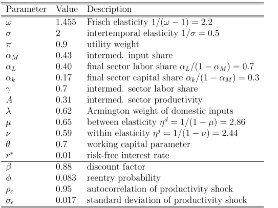
Given productivity ε and some specification of fiscal policy (τ, g), factor allocations, factor prices and output in a competitive equilibrium can be determined from the above conditions. In order to quantify the output costs of default, numerical values must be assigned to the model parameters. Our assignment, detailed in Table 1, introduces π as a new parameter but is otherwise identical to the one in Mendoza and Yue (2012) who calibrate their model to data from Argentina (1980Q1 - 2005Q4). Parameters below the line are relevant only to the full dynamic model discussed in Section 4.
3
Output costs of default in partial equilibrium
In order to assess the importance of fiscal policy for the determination of the output costs of default, we subject the model economy to a comparative experiment under an exogenous, possibly suboptimal debt policy (cf. the ‘partial equilibrium’ exercise in Section III of Mendoza and Yue, 2012). Given an amount b of maturing debt and the issuance of new debt b0, taxes and spending must satisfy the government budget constraint, τ c =g+ (1−d)[b−qb0], where
Table 1: Parameter values Parameter Value Description
ω 1.455 Frisch elasticity 1/(ω−1) = 2.2
σ 2 intertemporal elasticity 1/σ= 0.5
π 0.9 utility weight
αM 0.43 intermed. input share
αL 0.40 final sector labor share αL/(1−αM) = 0.7
αk 0.17 final sector capital share αk/(1−αM) = 0.3
γ 0.7 intermed. sector labor share
A 0.31 intermed. sector productivity
λ 0.62 Armington weight of domestic inputs
µ 0.65 between elasticity ηd= 1/(1−µ) = 2.86
ν 0.59 within elasticityηj = 1/(1−ν) = 2.44
θ 0.7 working capital parameter
r∗ 0.01 risk-free interest rate
β 0.88 discount factor
φ 0.083 reentry probability
ρε 0.95 autocorrelation of productivity shock
σ 0.017 standard deviation of productivity shock
d∈ {0,1}is a default indicator andqdenotes the price for sovereign debt placed on international financial markets. Substituting from (1), the government budget constraint can be rewritten as
τ
1 +τ =
g+ (1−d)1+r∗r∗¯b
gdp , (5)
where 1+r∗r∗¯b denotes the debt interest burden when a stationary level of debt ¯b is rolled over at
the risk-free world interest rater∗. This is actually without loss of generality: What matters for the determination of taxes and spending are not interest rates and debt separately, but only the resulting debt interest burden.5 Conditional on r∗
1+r∗¯b, (5) therefore captures the implications
for taxes and spending under any admissible debt policy. We then have the following result, which extends that of Cuadra, Sanchez, and Sapriza (2010) to an environment with endogenous
5Consider, e.g., the generic situation faced by a distressed country in the run-up to a default event. Elevated
interest rates then often induce the sovereign to consolidate its debt. But despite this fiscal consolidation prior to the default, the effective debt interest burden facing the country can still be appropriately represented by the expression in (5). In other words, the assumed stationarity of debt does not matter. By contrast, what matters is the endogeneity of the sovereign default decision itself, which we take as given in the partial equilibrium exercise at hand. Section 4 considers the full model where both debt dynamics and the government’s default decision are endogenous.
default costs along the lines of Mendoza and Yue (2012).
Proposition 1. Given some debt policy, the government’s optimal tax and spending policy is characterized by uc ( −∂ 1 1+τ ∂τ gdp ) =ug ( −∂ 1 1+τ ∂τ gdp+ τ 1 +τ ∂gdp ∂τ ) , (6)
which implies underprovision of public spending, uc< ug.
Given a debt interest burden of 3% of GDP, the preference weight π = 0.9 has been chosen such as to induce a level of public spending of 15% of GDP when the government honors its liabilities and productivity is at ε = 1. These numbers correspond roughly to their empirical counterparts in Argentina. Starting from there, we compare the output of final goods under default (yd) and repayment (ynd) for varying productivity. The output costs of default are then computed as 1−yd/ynd, whereby we contrast between three alternatives that differ in the fiscal adjustment in response to changing productivity and the exogenous repayment decision:
(i) the repayment regime (d= 0) where bothτ andg are adjusted optimally in line with (6); (ii) the default regime (d= 1) where both instruments are again adjusted optimally;
(iii) the default regime (d= 1) where one of the fiscal instruments is constrained to replicate the state-contingent level chosen in regime (i) while the other one must adjust residually to satisfy (5).6
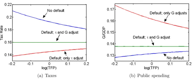
The differences across fiscal regimes are most readily seen in the two panels of Figure 1, which plot the tax rateτ and the level of public spending relative to GDP,g/gdp, against productivity. Under repayment, τ is decreasing in ε, while g/gdp is increasing. The reason is that higher productivity induces a higher tax base, which allows a more favorable reallocation from private to public consumption by means of taxation. By comparison, in regime (ii) τ is lower but
g/gdp is higher for all productivity states. This is because of the fiscal relief coming from
6This scenario arguably captures elements of fiscal sluggishness or other politico-economic considerations
which prevent the optimal fiscal accommodation of sovereign default. The specification with state-contingent replication of the repayment regime (i) is chosen because it facilitates a clean comparison with the results in Mendoza and Yue (2012). In Section 4, we instead consider model variants where either taxes or spending are fixed at a constant level.
(a) Taxes (b) Public spending
Figure 1: Fiscal instruments under different modes of fiscal adjustment
sovereign default. For the same reason, since tax revenues are no longer needed to finance the debt interest burden but used exclusively to provide public spending, both τ and g/gdp are now independent of ε.7 Finally, fiscal relief through default is also present in regime (iii), but there are two distinct cases. When only taxes adjust (panel (a)), τ is lower than in regime (i) and increasing in ε. When only spending adjusts (panel (b)), g/gdp is higher than in regime (i) and decreasing in ε.
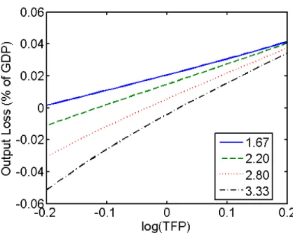
What does this imply for the output costs of default? Figure 2 plots these costs, contrasting the different scenarios for fiscal adjustment. We begin with the case of regime (iii) when taxes
Figure 2: Output costs of default under different modes of fiscal adjustment
7That τ and g/gdp are constant follows from the absence of wealth effects under GHH-preferences and
the fact that public expenditures and the consumption-leisure composite are subject to the same curvature parameterσ.
remain unchanged so that fiscal adjustment is exclusively in the form of changes in public spending. The resulting output costs of default are identical to those obtained in the model without fiscal policy studied by Mendoza and Yue (2012). This is because tax distortions are kept constant, while public spending enters utility in an additively-separable fashion and hence does not affect allocations. Next, consider the case of regime (iii) when public expenditure is fixed and fiscal adjustment comes entirely in the form of tax changes. Compared to the other case – and thus also to the model without fiscal policy – the output costs of default are lower, and for sufficiently low productivity shocks even negative; moreover, the output costs schedule is now steeper in ε. These two features are again due to the fact that debt repudiation through default relaxes the government budget constraint so that tax distortions are reduced. The relevance of this mechanism is higher in low productivity states because the underlying tax base is smaller so that default allows for a greater reduction of the tax rate. Finally, regime (ii) where both instruments are adjusted optimally generates output costs of default that average out the previous two scenarios both in terms of level and slope.
As seen, the consideration of fiscal policy in general, and the specification of details about the fiscal adjustment process in particular, have quantitatively relevant implications for the output costs of default. Fiscal activity matters due to its distortionary effect on labor supply. It is therefore interesting to examine the sensitivity of our findings to changes in the elasticity of labor supply ω−11.8 Figure 3 does this for regime (ii) where both fiscal instruments are adjusted optimally. In Mendoza and Yue (2012), a higher elasticity of labor supply dampens the wage response in the event of default, which implies stronger intersectoral reallocation effects and ultimately higher output costs of default. This comparative-static effect is actually reversed once fiscal policy is taken into account: a higher Frisch elasticity is now associated with lower (possibly even negative) output costs of default. To understand this, recall that default induces lower tax rates (cf. Figure 1). This has a positive effect on labor supply which is more pronounced the higher the elasticity of labor supply. In addition to their level effect on the output costs of default, induced changes in taxation can hence also affect important qualitative lessons from the model where fiscal policy is absent.
8The key role of the substitution elasticitiesηd= 1 µ−1 andη j= 1 ν−1
as determinants of the output costs
of default already pointed out by Mendoza and Yue (2012) is preserved also in our modified model with fiscal policy.
Figure 3: Regime (ii): Output costs of default under different labor supply elasticity
4
Full model with endogenous debt and default
In light of the partial equilibrium findings discussed in Section 3, we now proceed to examine the implications of endogenous fiscal policy in the context of the full model where debt dynamics, interest rate spreads and sovereign default all arise endogenously. This approach is important for the appropriate quantification of the induced output costs of default for a number of rea-sons. First, it endogenizes the economy’s external debt position and its pricing via sovereign spreads at the time of default and thus allows to assign a model-consistent magnitude to the relevant debt interest burden in (5). Second, since the government’s incentive to exercise its default option varies not only with the level of inherited debt b, but also with the economy’s productivity state ε, an empirically relevant measure of the output costs of default should take into account its endogenous occurrence over the business cycle. This is important since the sovereign government’s underlying cost-benefit assessment is necessarily relative to the alter-native means of fiscal adjustment other than outright sovereign default. Finally, the analysis of the full model facilitates a comprehensive sensitivity analysis of the deeper determinants of the output costs of default while taking account of intertemporal dynamics and adjustment.
The full model’s intertemporal properties are determined by the parameters below the line in Table 1, (β, φ, ρε, σ): the government’s discount factor β, the process for market exclusion following default, and the law of motion for productivity. Default wipes out the entirety of the government’s outstanding debt at the cost of financial autarky, that is, exclusion from international credit markets. When in bad credit standing, the government may regain access
to international credit markets in the next period with an exogenous probability φ. Its default decision therefore trades off the costs of the resource transfer to international creditors under repayment against the costs of temporary market exclusion given by the foregone benefits of consumption smoothing and the output loss in autarky due to the non-availability of working capital to firms.
The government’s intertemporal problem can be expressed in recursive form. Let V(b, ε) denote the value function of the government. Its optimal default decisiond(b, ε)∈ {0,1}solves the following problem,
V(b, ε) = max d
Vnd(b, ε),Vd(ε) , (7)
where Vnd(b, ε) and Vd(ε) are the value functions conditional on repayment and default, re-spectively. The government problem conditional on repayment is
Vnd(b, ε) = max
τ,g,b0 {u(c−v(L), g) +βEV(b
0, ε0)} (8)
subject to g = τ c+q(b0, ε)b0 −b and the relevant private-sector equilibrium conditions when working capital loans are available (κ >0). By contrast, the problem of a defaulting government is Vd(ε) = max τ,g u(c−v(L), g) +βE (1−φ)Vd(ε0 ) +φV(0, ε0) (9)
subject to g =τ cand the private-sector equilibrium conditions when working capital loans are not available (κ = 0).
Throughout, the government discounts future values with the factor β ∈ (0,1), and forms expectations over future productivity in final goods productionε0. The underlying productivity shocks are assumed to follow an AR(1) process,
lnε0 =ρεlnε+0,
risk-neutral and determine bond prices. Facing an opportunity cost of funds equal to r∗, they invest in one-period sovereign bonds and in within-period private working capital loans. Competition implies that lenders expect zero profits and that the returns on sovereign debt and the world’s risk-free asset are fully arbitraged. Bond prices are then given by
q(b0, ε) =E 1−d(b0, ε0) 1 +r∗ . (10)
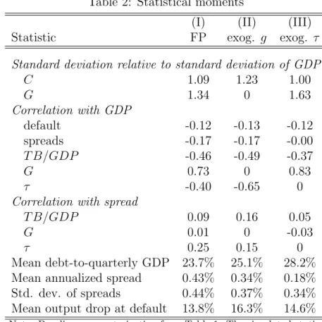
Notice that the solution to the government problem in (7), (8) and (9) supports the char-acterization of the optimal tax and spending policy in Proposition 1. Similarly, and regardless of the specification of fiscal policy, the optimal debt policy is driven by the pricing of default risk in (10) and hence procyclical. Table 2 in the Appendix reports the induced business cycle statistics of the model, parameterized as in Table 1, in greater detail. Similar to the partial equilibrium analysis in Section 3, we contrast between three alternative models, which, however, all feature endogenous debt dynamics and default:
(i) the benchmark model where both τ and g are adjusted optimally in each period; (ii) the model where g remains fixed and τ adjusts optimally;
(iii) the model where τ remains fixed and g adjusts optimally.
Of particular interest is the average output drop at default, which is at 13.8% in the benchmark model (i), at 16.3% in model (ii), and at 14.6% in model (iii).9 In terms of broad macroeconomic outcomes, our model versions with fiscal policy are thus roughly aligned with one another and also with the results reported in Mendoza and Yue (2012). However, notable differences become apparent when we further scrutinize the default events realized in the alternative model environments.
4.1
Default dynamics with fiscal policy
In all three alternative models with fiscal policy, output costs of default emerge as a consequence of two competing effects. On the one hand, default induces a misallocation of resources due
9In the model without fiscal policy considered by Mendoza and Yue (2012), the output drop at default is at
to the unavailability of working capital loans for imported intermediate inputs – the working capital channel. On the other hand, due to the fiscal relief through default there is potential scope for tax cuts with favorable effects on labor supply – the tax channel.
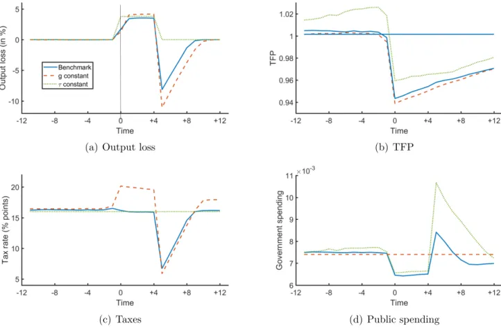
Figure 4 depicts results from the simulation of the three alternative models, with a focus on macroeconomic dynamics around recorded default episodes. The timing of defaults is normal-ized to occur att = 0. While the process for regaining access to financial markets is stochastic, the plotted series condition on reentry att = 5. Panel (a) considers the output costs of default
(a) Output loss (b) TFP
(c) Taxes (d) Public spending
Figure 4: Macroeconomic dynamics and default costs under different fiscal regimes. The dis-played values are computed as averages over N=50.000 simulations of length T=500 with the first 100 observations truncated.
induced for the three alternative models. Notice first that the output costs of default, again computed as 1−yd/ynd, are conceptually different from the output drop at default mentioned above. The output drop at default compounds the output costs of default with the adverse productivity dynamics driving the economy into sovereign default; see panel (b). By contrast,
the output costs of default isolate thedirectconsequences of default through the working capital and tax channels relative to the counterfactual with repayment.
Model (iii) with exogenous taxes, kept constant at τ = 0.16, allows for the most straightfor-ward interpretation. Since taxes remain unchanged both throughout the default episode and relative to the counterfactual with repayment, the output costs of default materialize through the working capital channel only and are constant throughout the exclusion period at about 4%. They then revert to zero when the economy again gains access to international credit markets in t= 5.
In the other models, which feature variation in taxes, the output costs of default are sub-stantially lower on impact (t= 0) at around 1.5%. This reflects the additional fiscal relief from default, which allows for lower taxes and hence boosts labor supply. Importantly, however, this advantage plays out not in absolute terms but only relative to the counterfactual with repayment. Indeed, panel (c) shows that, initially, taxes hardly move in the benchmark model (i) and even need to be raised in model (ii) with exogenous spending. Notice also that the fiscal relief is transitory as the government benefits from debt repudiation only initially (t= 0) and must then run a balanced budget throughout the exclusion period. This implies that the output costs of default increase beyond their moderate level in t = 0 and from t = 1 onwards approximately reach the 4% level experienced also in model (iii) with constant taxation (slightly less for model (i) and slightly more for model (ii)).10
Finally, upon gaining access to international credit markets int= 5, the variable-tax models (i) and (ii) see a pronounced drop in taxation, which materializes in terms of substantial output gains (again, relative to the counterfactual with repayment). This reentry-boom is entirely tax driven and is therefore neither present for model (iii) with constant taxes nor for the model without fiscal policy studied by Mendoza and Yue (2012).
10To understand the discussed output costs of default correctly, it is also important to realize that the generic
TFP dynamics driving the government into default differ across the three models. As seen from panel (b), defaults in the benchmark model (i) arise as a consequence of a sudden drop in TFP from average levels by about one standard deviation (−5.7%). While the process for model (ii) with exogenousgis similar, model (iii) with exogenousτ starts from a pre-default boom followed by a drop in productivity to a level about 4% below the unconditional average. The differential TFP dynamics indicate that alternative regimes for fiscal policy are not neutral for the endogenous selection into default. This matters for the output costs of default because they are increasing in the level of productivity (cf. Figure 2).
4.2
Working capital channel versus tax channel
As explained above, the output costs of default recorded in Figure 4 reflect the interplay between the working capital channel and the tax channel. An important qualitative finding from the partial equilibrium analysis in Section 3 is that, in contrast to the model without fiscal policy, the output costs of default are decreasing in the elasticity of labor supply ω1−1. This reversal emerges because the output effects of both the working capital channel and the tax channel are increasing with the Frisch elasticity, whereby the latter proves more powerful in the comparative experiment underlying Figure 3. This result remains robust also in the full quantitative model with endogenous debt and default.
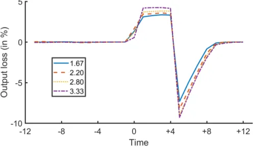
Figure 5 displays the output costs of default induced in the benchmark model (i) under alternative parameterizations for the elasticity of labor supply. Indeed, conditioning on the
Figure 5: Output costs of default for the benchmark model with endogenous taxes and spending under different labor supply elasticity. The displayed values are computed as averages over N=50.000 simulations of length T=500 with the first 100 observations truncated.
impact period of default (t = 0) when both the working capital channel and the tax channel are active, the Figure shows that a higher Frisch elasticity is associated with lower (but unam-biguously positive) output costs of default, ranging from 1.6% when ω1−1 = 1.67 to 0.5% when
1
ω−1 = 3.33. The tax channel thus dominates the working capital channel in its interaction with the elasticity of labor supply. However, the output costs of default again change over time due
to the fact that the fiscal relief from default is transitory. As a consequence, fromt= 1 onwards the output costs of default increase considerably to levels in the range of 3% to 4%. Moreover, since the tax channel ceases to be relevant, the ranking across the different parameterizations now indicates that the output costs are increasing with the Frisch elasticity, in line with the working capital channel.
In sum, the analysis of the quantitative model therefore delivers a number of important findings. First, the margin of fiscal adjustment has important consequences for the magnitude of the output costs of default and their dynamic pattern during the period of market exclusion. Second, for the range of labor supply elasticities considered sovereign default results in output losses relative to the counterfactual with repayment.11 And third, as long as the tax channel is active these output costs are actually decreasing in the Frisch elasticity. This qualitative difference to the model without fiscal policy is important for the assessment of default incentives when labor market dynamics play an important role.
5
Conclusions
This note introduces fiscal policy into a sovereign debt model with endogenous default costs and examines the implications for the determination of the output costs of default. We find that the quantitative properties of the output costs of default, and their dependence on primitives such as the elasticity of labor supply, are distinctly different depending on the margin of fiscal adjustment. These results emerge from a partial equilibrium analysis of three distinct regimes under an exogenous debt and default policy, but are preserved also in the full quantitative model with variations in bond prices that induce endogenous cyclical dynamics in the government’s debt, tax, spending and default policy. The consideration of fiscal policy thus has potentially important implications for the quantitative properties of models of sovereign debt and default. While the focus of this note is on the output costs of sovereign default, our analysis suggests that the magnitude of the tax channel and its incidence over time are particularly relevant driving forces. The model at hand considers one-period debt and hence features only relatively
11Recall that the direct output costs of default must be compounded with the output effects due to the
underlying productivity dynamics to get the complete, empirically relevant measure for the output drop at default.
moderate debt levels. In future work, it might therefore be interesting to consider models of long-term bonds with positive debt recovery rates after default.
References
Aguiar, M., and G. Gopinath (2006): “Defaultable debt, interest rates and the current
account,”Journal of International Economics, 69(1), 64–83.
Arellano, C. (2008): “Default Risk and Income Fluctuations in Emerging Economies,”
American Economic Review, 98(3), 690–712.
Balke, N. (2017): “The employment cost of sovereign default,” mimeo, University College
London.
Borensztein, E., and U. Panizza (2009): “The Costs of Sovereign Default,” IMF Staff
Papers, 56(4), 683–741.
Cuadra, G., J. Sanchez, and H. Sapriza (2010): “Fiscal Policy and Default Risk in
Emerging Markets,” Review of Economic Dynamics, 13(2), 452–469.
De Paoli, B., G. Hoggarth, and V. Saporta (2009): “Output costs of sovereign crises:
some empirical estimates,” Bank of England working papers 362, Bank of England.
Eaton, J., and M. Gersovitz (1981): “Debt with Potential Repudiation: Theoretical and
Empirical Analysis,” Review of Economic Studies, 48(2), 289–309.
Greenwood, J., Z. Hercowitz, and G. W. Huffman (1988): “Investment, Capacity
Utilization, and the Real Business Cycle,” American Economic Review, 78(3), 402–17.
Mendoza, E. G., andV. Z. Yue(2012): “A General Equilibrium Model of Sovereign Default
and Business Cycles,” The Quarterly Journal of Economics, 127(2), 889–946.
Na, S., S. Schmitt-Groh´e, M. Uribe, and V. Z. Yue (2014): “The Twin Ds: Optimal
Default and Devaluation,” NBER Working Papers 20314, National Bureau of Economic Research, Inc.
Niemann, S., and P. Pichler (2017): “Optimal fiscal policy and sovereign debt crises,”
Panizza, U., F. Sturzenegger, and J. Zettelmeyer (2009): “The Economics and Law
of Sovereign Debt and Default,”Journal of Economic Literature, 47(3), 651–98.
Tavares, T. (2015): “Labor Market Distortions under Sovereign Default Crises,” MPRA
Paper 66964, University Library of Munich, Germany.
Vegh, C. A., and G. Vuletin (2015): “How Is Tax Policy Conducted over the Business
A
Appendix
A.1
Optimal tax and spending policy
Proof of Proposition 1. Given some debt policy, the optimal tax and spending policy must satisfy (5) and uc ∂c ∂τ −ul ∂L ∂τ +ug ∂g ∂τ = 0.
Using (1) and (2), the optimality condition for taxes becomes
0 = uc "∂gdp ∂τ (1 +τ)−gdp (1 +τ)2 # −ucv0(L) ∂L ∂τ +ug " (gdp+τ∂gdp∂τ )(1 +τ)−τ gdp (1 +τ)2 # , or equivalently, uc ( −∂ 1 1+τ ∂τ gdp− 1 1 +τ ∂gdp ∂τ +v 0 (L)∂L ∂τ ) =ug ( −∂ 1 1+τ ∂τ gdp+ τ 1 +τ ∂gdp ∂τ ) .
From the definition of GDP as the value of the output of final goods net of the costs of imported intermediate inputs, gdp=y−P∗(r∗)m∗, and since factors earn their marginal products, while the price for imported inputs is exogenous, we have
∂gdp ∂τ = ∂gdp ∂L ∂L ∂τ + ∂gdp ∂m∗ ∂m∗ ∂τ =w ∂L ∂τ + [P ∗ (r∗)−P∗(r∗)]∂m ∗ ∂τ =w ∂L ∂τ.
Hence, the optimality condition for consumption-leisure (2) implies
− 1 1 +τ ∂gdp ∂τ +v 0 (L)∂L ∂τ = − w 1 +τ ∂gdp ∂τ +v 0 (L) ∂L ∂τ = 0,
so that the the optimality condition for taxes becomes
uc ( −∂ 1 1+τ ∂τ gdp ) =ug ( −∂ 1 1+τ ∂τ gdp+ τ 1 +τ ∂gdp ∂τ ) .
This condition has an interpretation in terms of marginal benefits and marginal costs of chang-ing the tax rate. Accordchang-ingly, variations in the government’s tax policy are seen to have two effects: a direct reallocation effect (−∂
1 1+τ
∂τ gdp >0), and a budgetary effect ( τ 1+τ
∂gdp
∂τ < 0). In detail, for given GDP, an increase in the tax rate allows to reallocate resources from private to public consumption. However, this causes tax distortions which work to reduce GDP, the relevant tax base for the consumption tax, and thus has negative implications for the govern-ment’s budget. In conjunction, this implies that the optimal fiscal policy limits distortions by keeping public expenditure below its first-best level, that is, uc < ug.
A.2
Business cycle implications under different fiscal policies
Table 2: Statistical moments
(I) (II) (III)
Statistic FP exog. g exog. τ
Standard deviation relative to standard deviation of GDP
C 1.09 1.23 1.00 G 1.34 0 1.63 Correlation with GDP default -0.12 -0.13 -0.12 spreads -0.17 -0.17 -0.00 T B/GDP -0.46 -0.49 -0.37 G 0.73 0 0.83 τ -0.40 -0.65 0
Correlation with spread
T B/GDP 0.09 0.16 0.05
G 0.01 0 -0.03
τ 0.25 0.15 0
Mean debt-to-quarterly GDP 23.7% 25.1% 28.2%
Mean annualized spread 0.43% 0.34% 0.18%
Std. dev. of spreads 0.44% 0.37% 0.34%
Mean output drop at default 13.8% 16.3% 14.6%
Note: Baseline parameterization from Table 1. The simulated statis-tics are computed as averages overN = 20.000 simulations of length
T = 500, with the first 100 observations truncated. The simulated series are logged and filtered.