Mulvey, D., Foh, C. H., Imran, M. A. and Tafazolli, R. (2018) Cell Coverage
Degradation Detection Using Deep Learning Techniques. In: 2018 International
Conference on Information and Communication Technology Convergence (ICTC), Jeju
Island, Korea, 17-19 Oct 2018, pp. 446-447. ISBN 9781538650417.
There may be differences between this version and the published version. You are
advised to consult the publish
er’
s version if you wish to cite from it.
http://eprints.gla.ac.uk/168096/
Deposited on: 3 September 2018
Enlighten
–
Research publications by members of the University of Glasgow
Cell Coverage Degradation Detection Using Deep
Learning Techniques
David Mulvey[1], Chuan Heng Foh [1], Muhammad Ali Imran [2], and Rahim Tafazolli [1]
[1] 5G Innovation Center, Institute for Communications Systems, University of Surrey
[2] School of Engineering, University of Glasgow
Abstract—This article presents the results of an investigation of the application of deep learning techniques to the sleeping cell problem, in order to achieve greater detection sensitivity than previously reported.
We use a deep recurrent Neural Network (rNN) to process simulated RSRP reports in order to detect degradations of cell radio performance as well as complete outages. Using such a configuration we are able to achieve improved sensivity in relation to a traditional Support Vector Machine (SVM) approach, while eliminating the need for a separate dimensionality reduction stage at the front end. We study multiple rNN configurations with up to three hidden layers and conclude that in this scenario we can achieve the target improvement in sensitivity with a single hidden layer, leading to highly efficient run time performance.
Index Terms—Cellular networks, self healing, cell outage, cell degradation, fault detection, deep learning, neural networks
I. INTRODUCTION
T
HE network architecture for 5G has evolved significantly in comparison with 4G. The Radio Access Network (RAN) architecture has become more decentralised, with a new two tier architecture in which user traffic is now devolved to groups of small cells under the control of a single macrocell [1], [2], [3].In the new RAN architecture, extensive use is made of Multi User Multiple Input Multiple Output (MU-MIMO) techniques combined with Coordinated MultiPoint (CoMP) transmission methods [4]. Three dimensional propagation techniques based on planar array techniques are being used to maximise signal strength in built up areas, especially in high rise locations [5]. Deployment of these techniques in 5G will require a dra-matic increase in the number of configuration parameters required in comparison with 4G, with a corresponding increase in the likelihood of misconfiguration.
With the advent of very large numbers of small cells, new resilience and load balancing techniques will be required to optimise resilience and energy consumption in situations where the numbers of users in a given cell may vary from full capacity to zero over a 24 hour period. It will become uneconomic to make a site visit to fix a single cell so it will be necessary for the network to compensate for faults so that multiple physical faults can be resolved during a single visit. Such increases in complexity will require additional auto-mated assistance to network operations centre staff, to allow them to focus on key issues rather than being overwhelmed by detail. This has led to considerable interest in how machine
Manuscript received August 31, 2018; revised tbc.
learning (ML) techniques can be used to detect faults quickly and even compensate for certain faults until a permanent fix can be provided.
A key problem which is specific to radio networks is the so-called sleeping cell issue, where a fault occurs somewhere in the radio frequency transmission chain leading to users experiencing an outage which, however, is not visible to the network management team.
To date, ML approaches have been successfully used to detect complete outages of a cell from indirect evidence such as reports from user equipment and neighbouring cells. Key techniques of choice at the current time include k nearest neighbour anomaly detection and support vector machines used as binary classifiers.
At the current state of the art, however, such techniques typically depend on a hand-engineered data preprocessing stage to reduce the dimensionality of the data so that it can be efficiently processed by the ML system, and are capable of detecting complete outages but are not necessarily able to identify more subtle radio signal degradations.
Research in other engineering areas with similar issues [6] has shown that deep learning techniques can process large numbers of input data features without the need for a hand-engineered input stage. We therefore decided to apply a deep learning approach to the cell coverage degradation detection problem. For this work we have chosen to use a recurrent neural network (rNN), because of its inherent ability to handle time based sequences, enabling us to take into account events leading up to a fault if appropriate.
In this paper we make the following three contributions: firstly we show that we can use an rNN to build a more sensitive fault detector than feasible with a support vector machine (SVM) ; secondly that we can eliminate the hand coded data dimensionality reduction stage required by the SVM by exploiting the ability of the rNN to process input data directly; and thirdly that we can utilise the ability of the rNN to process large numbers of input channels to allow us to use a single hidden layer rNN configuration, minimising the need for run time computing power.
This paper is organised as follows. First we present related work in this area and discuss the strengths and limitations of the current state of the art. Next we outline the architecture of the rNN in the context of current deep learning techniques, and describe the simulation we used to train and test it. Finally we present and discuss our results and offer some suggestions for further work.
II. RELATEDWORK
Recent studies have made extensive use of measurement data reported by the user equipment as a result of the Minimise Drive Testing (MDT) initiative, designed to reduce the amount of expensive drive testing needed to verify radio coverage. Typical KPIs relevant to sleeping cell detection include Refer-ence Signal Received Power and Quality (RSRP/Q) from the cell being monitored and the neighbouring cells, as well as the wideband Channel Quality Indicator (CQI) for the cell being monitored.
The number of parameters required for effective detection may be more than the optimal number of inputs to the ML system, in which case a dimensionality reduction strategy will have to be used, such as the MultiDimensional Scaling (MDS) approach used by many of the sleeping cell studies.
Machine learning techniques applied to the sleeping cell detection problem during the last five years may be split into two major classes: parametric and non parametric methods. Both use training data to learn from; the difference is in how they use it. Parametric methods fit a model to the training data during a training phase, then use the model to make predictions from live data during a subsequent operational phase. Non-parametric methods, on the other hand, do not require a training phase but instead use the training data directly during the operational phase when forming a prediction.
In both cases the training data has to be labelled by an expert as normal or anomalous. To reduce the cost of this, a front end clustering algorithm [7] can be used to partition the data into clusters so that the expert only has to confirm the labels of the clusters rather than label the data in detail.
Studies utilising parametric techniques [8] CLNS2013 and [9] ZSIIA2015 have made use of the SVM approach, in which an anomaly boundary is set during the training phase so that it can be used to classify whether data is normal or anomalous during the operational phase.
Studies using non-parametric techniques [9] ZSIIA2015, [10] XPMZ2014, [11] WPP2016, [12] XZLLP2014 [13] OZMIGID2015 and [14] CCBR2015 [15] typically use either a variation of the k Nearest Neighbours technique or a similar approach, in which a measure of the distance, or dissimilarity, between neighbouring data items is used to compare an incoming data item with its nearest neighbours in the training set, which have already been labelled as normal or anomalous. Quantitative comparisons between methods are hindered by the lack of a standard reporting approach, but for those studies using the receiver operating curve (ROC) graph, the best reported figures for SVMs claim a true positive rate (TPR) in the region 85%-90% at a false positive rate (FPR) of 10% [9], and for kNN the best TPR is reported to be in the region of 80% for a similar FPR [13].
Both the SVM and the kNN techniques have the limitation that a significant amount of preprocessing of the input data is required, including dimensionality reduction, requiring dedi-cated code which can be inflexible as well as expensive to set up and maintain.
All the above techniques consider each live data point sepa-rately, without any consideration of any relationships between
successive data items which form a sequence (as do successive values of the KPIs listed above). Several studies have included an element of time series prediction [8] CLNS2013 (ARIMA modelling), [13] OZMIGID2015 (Grey modelling), and [16] ZLP2014 (adaptive filtering), but these require specialist code to implement each method rather than making use of a general purpose ML technique.
III. DEEPLEARNING FORDEGRADATIONDETECTION A different type of ML approach, neural networks (NNs), is proving very effective in other domains with similar challenges to those of mobile networks. NNs consist of a set of nodes, each of which applies a specific linear weighting to each of its inputs, followed a non-linear transformation to compress the result. Nodes are typically organised in layers, providing input and output and also often including internal or hidden layers.
In the feedforward NN, each variable at each stage is weighted with its own individual weight. Once the network is trained, the output depends only on the current inputs. In the recurrent NN (rNN), by contrast, the network maintains an internal state derived from the previous input. This allows it to operate on a sequence of inputs taking into account any relationships between the current input and previous ones.
Networks with more than one hidden layer, known as deep NNs, have proved themselves very effective in detecting faults and degraded performance in other complex engineering systems, and have demonstrated the ability to eliminate much of the hand coded front end processing previously required for this type of application [17], [18] and [19].
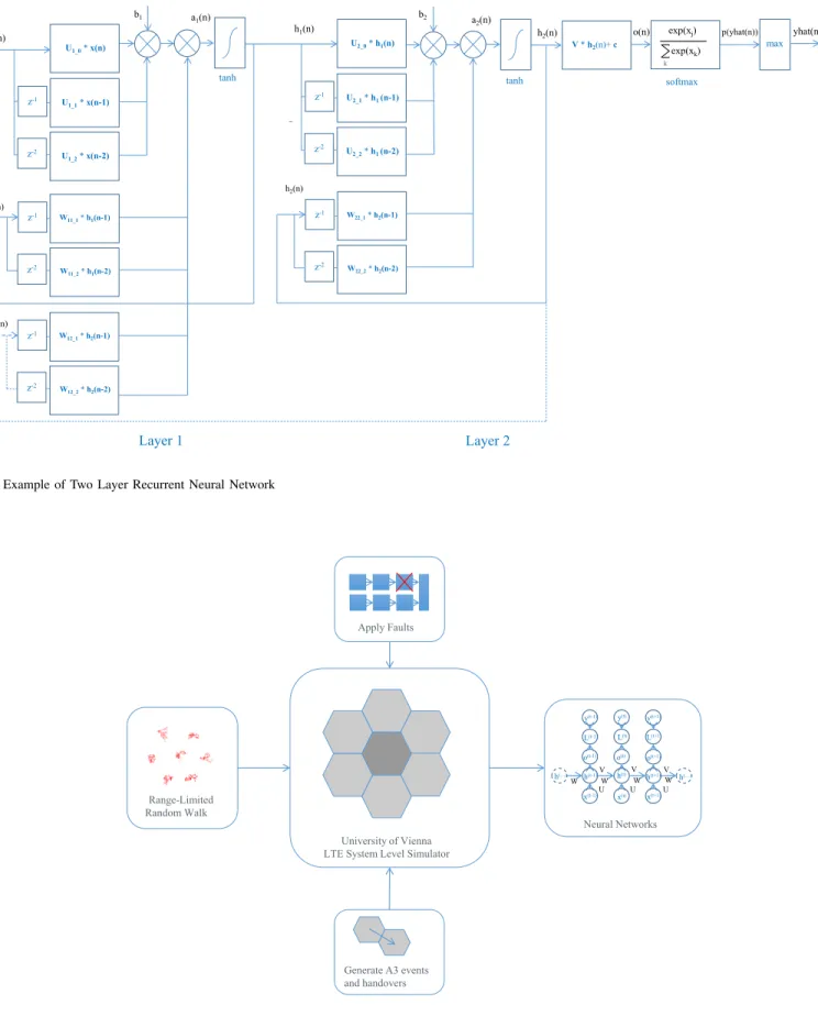
Hence our aim is to apply a deep NN to the sleeping cell problem with the goal of improving detection sensitivity and reducing the amount of front end coding required compared with current methods. For this work, we have used an rNN (see Fig 1) operating on a series of fixed length sequences taken from the input data. This method has a number of advantages for this scenario in comparison with classic ML approaches and other NN techniques.
Firstly, it is able to take into account dependencies between features in the current data input set and those in previous inputs. So if there were a precursor event just before a fault, for example, the rNN would be able to exploit this.
Secondly, the rNN’s ability to represent time or sequential dependencies provides the option to learn to filter the input, perhaps to reduce noise (low pass filtering) or to accentuate transitions (high pass filtering).
Thirdly, the rNN shares its parameters across all data items in a sequence. Consider a set of n examples, each representing a sequence of s values of p features. The rNN requires input data to be presented as a vector of p features at a time, for each of the s values in the sequence for each of n examples. Classic techniques such as the SVM and other neural network approaches such as the feedforward NN, on the other hand, would require s x p values to be presented in parallel for each example, requiring of order s times as many parameters to be trained.
The classic rNN described in the textbooks [20] derives its internal state from the previous input only. We have extended
a1(n) x(n) h1(n) tanh U1_1* x(n-1) U1_0* x(n) U1_2* x(n-2) z-1 z-2 h1(n) W11_1* h1(n-1) W11_2* h1(n-2) z-1 z-2 h2(n) W12_1* h2(n-1) W12_2* h2(n-2) z-1 z-2 h2(n) o(n) p(yhat(n)) a2(n) tanh V* h2(n)+ c softmax exp(xk) exp(xj) k U2_1* h1 (n-1) U2_0* h1(n) U2_2* h1 (n-2) z-1 z-2 W22_1* h2(n-1) W22_2* h2(n-2) z-1 z-2 h2(n) b2 b1 Layer 1 Layer 2 max yhat(n)
Fig. 1. Example of Two Layer Recurrent Neural Network
University of Vienna LTE System Level Simulator Range-Limited Random Walk Neural Networks W V U y(t-1) L(t-1) o(t-1) h(t-1) x(t-1) y(t+1) y(t) L(t) L(t+1) o(t) o(t+1) h(t) h(t+1) h(…) h(…) x(t) x(t+1) W W W U U V V Apply Faults Generate A3 events and handovers
this architecture to allow processing of up to four previous inputs with a single hidden layer, and up to two previous inputs with up to four hidden layers. An example of this architecture configured for two hidden layers and processing of two previous inputs is shown in Fig 1. We also introduce an input filtering layer fully integrated into the rNN, with the filter parameters learned as part of the rNN training process. This allows the rNN to filter the input features in whatever way it learns to be optimal in order to achieve the maximum accuracy.
Once implemented, the rNN is then trained, validated and tested against a network simulation as described in the next section.
IV. SYSTEMSIMULATION TABLE I
SIMULATORCONFIGURATIONDETAILS
Configuration
Element Settings eNodeBs Hexagonal grid
Central eNodeB surrounded by one ring of 6 Inter eNodeB distance 200m
Tx power 41dBm Radio
Propagation Model
Pathloss model 3D TR36.873 [21] Channel model 3D-UMi
Minimum coupling loss 70dB Street width 20m, building height 20m Radio Link Frequency 2000MHz, Bandwidth 10MHz
4 x Tx, 4 x Rx
Transmission Mode 4 (Closed Loop Spatial Multiplexing)
UEs 21 UEs, initial allocation 3 per eNode B User Walking
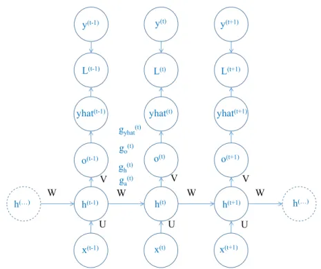
Model Random walk within 100m radius from basestation The network simulation is based on the LTE system level simulator built in MATLAB by the Technical University of Vienna (TUV). The model has been modified to provide a outer loop representing user movement on a timescale of minutes, with the radio simulation operating as an inner loop based on the LTE Transmission Time Interval (TTI) period. All modifications and extensions to the simulator are also implemented in MATLAB.
For simulation purposes, we assume a split cellular net-work architecture with the macrocell operating on a different frequency from the small cells. We model just the small cells, assuming that the network is fully planned, so that at present we do not consider the effect of unplanned femtocells.
In the model, a central cell is surrounded by a ring of six identical cells. Faults are applied to the central cell only. Users are assumed to be pedestrians and are each initially allocated to one of the small cells. User positions are generated by a range limited random walk model, added to the basic TUV simulator, where the user position is constrained to remain within a configurable radius of the starting point.
The simulator is configured to use a 3D propagation model according to 3GPP TR36.873 [21]. At initialisation time, the
simulator makes a random selection between Line of Sight (LOS) and Non Line of Sight NLOS propagation per eNodeB per mobile device, based on UE location. At the same point, the simulator makes a similar choice between in-building and external propagation for each location, in this case independent of UE.
We have added facilities to the TUV simulator to calculate RSRP and RSRQ levels, produce MDT reports and generate events such as A3 events and handovers which are derived from network states.
We present the output from the simulator in the form of simulated network MDT and RRC Measurement report data. We normalise the data from these and split it into training, validation and test data sets before passing it to the deep learning system.
V. DETECTORIMPLEMENTATION
Our investigation makes use of 9 simulated RSRP reports from mobile devices, three attached to the cell under investiga-tion and one attached to each of the surrounding cells. It should be noted that this figure was chosen based on a judgement as to the likely numbers of active users in a typical dense cell deployment - the number of RSRP inputs is not limited by the rNN and could be increased if the numbers of available users permit.
We compare the performance of the following detection techniques:
1) an rNN with a configurable number of hidden layers, extended to provide additional input and internal state filtering as described above.
2) an SVM with a radial basis function (RBF) kernel using hand coded MDS dimensionality reduction, designed to be representative of previous work in this field
In each case the sequence length is 20 samples; the system is trained on 144 examples of one sequence each, validated on 48 examples and tested on 48 examples.
A. Recurrent Neural Network
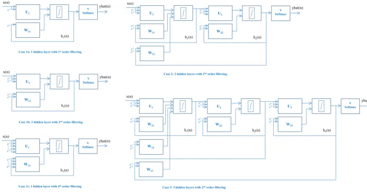
The structure of the basic rNN, unfolded over a typical sequence, is shown in the following figure.
The forward path is defined by the following equations [20] chapter 10, for stept within a given sequence:
at=b + Wht−1 + UXt ht =f(at) ot=c+Vht p!yˆt j " =sof tmax(otj) = exp(ot j) # kexp(o t k) f$at%=tanh$at% Lt= −#kln !ˆ yt k "
The back propagation path is defined by the following gradients (combined using the chain rule) based on the
W V U y(t-1) L(t-1) o(t-1) h(t-1) x(t-1) y(t+1) y(t) L(t) L(t+1) o(t) o(t+1) h(t) h(t+1) h(…) h(…) x(t) x(t+1) W W W U U V V go(t) gh(t) gyhat(t) ga(t)
yhat(t-1) yhat(t) yhat(t+1)
Fig. 3. Unfolded RNN Structure
principles given in [20] section 10.2.2:
∂Lt ∂yˆt j =−1 ˆ yt j ∂yˆt j ∂ot
i has two cases: f or i̸= j, ∂
ˆ
yt j
∂ot
i =−pjpiwhere pn=sof tmax
$ ot n % f or i= j, ∂ ˆ yt j ot i =−pj(1−pj) ∂c ∂ot = 1 ∂V ∂ot =ht ∂ht ∂ot =V ∂at ∂ht =diag $1 −ht2% [∂ ∂xtanh(x) = 1−tanh 2(x)] ∂b ∂at = 1 ∂W ∂at =ht−1 ∂U ∂at =Xt
The basic network is extended to allow processing of earlier values of the input and internal state, as far back as Xt−4
and ht−4respectively, with the necessary weighting parameters
fully integrated into the forward and back propagation paths. Similar code is used to extend the network to provide two or three hidden layers as required.
During the training phase, a regularisation parameter is used to select the best tradeoff between overfitting and underfitting
the machine learning parameters in relation to the training data. We systematically train the detection and diagnosis system against the training data using a range of values of lambda, then select the value of lambda which gives the best prediction accuracy on the validation data set. This value is then used to test prediction accuracy on the test set.
Prediction accuracy is measured by calculating true and false positive and negative prediction rates, expressed as a proportion of the total number of cases. Selection of the most appropriate value of the regularisation parameter is based on the sum of the true positive and true negative prediction rates. The following rNN configurations were implemented (see Fig 4):
1) a single hidden layer with options for first, second and fourth order filtering on both the internal states and the inputs (cases 1a-1c)
2) two hidden layers with second order filtering for the internal state and the inputs (case 2)
3) three hidden layers with second order filtering for the internal state and the inputs (case 3)
B. Support Vector Machine
The SVM implementation uses the MATLAB function
fitcsvm with the ’Kernelfunction’ and ’rbf’ options selected,
followed by thefitPosteriorfunction to convert the classifica-tion score to a probability.
Dimensionality reduction follows the method given in [9], in which the first step is to find the topmeigenvectorsV and eigenvaluesλofXTX . The required data set now containing
x(n) h1(n) U1 V Softmax yhat(n) W11 z-1 z-1 x(n) h1(n) U1 V Softmax W11 z-1 z-4 z-1 z-4 V Softmax x(n) h1(n) U1 W11 z-1 z-2 z-1 z-2 W13 W12 z-1 z-2 x(n) h1(n) U1 W11 z-1 z-2 z-1 z-2 V Softmax h3(n) U3 W33 z-1 z-2 z-1 z-2 h2(n) U2 W22 z-1 z-2 z-1 z-2 z-1 z-2 W12 z-1 z-2 x(n) h1(n) U1 W11 z-1 z-2 z-1 z-2 V Softmax h2(n) U2 W22 z-1 z-2 z-1 z-2
Case 1a: 1 hidden layer with 1storder filtering
Case 1b: 1 hidden layer with 2ndorder filtering
Case 1c: 1 hidden layer with 4thorder filtering
Case 2: 2 hidden layers with 2ndorder filtering
Case 3: 3 hidden layers with 2ndorder filtering
yhat(n) yhat(n)
yhat(n)
yhat(n)
Fig. 4. RNN Configurations
For comparability with [9] we set mto 3. If the MATLAB
eigsfunction is used to calculate the eigenvalues and vectors, it should be noted that this assigns a random sign to its output so code should be included to detect this and adjust the relevant signs as needed. The SVM uses the same approach to calculating the prediction accuracy as described above for the rNN.
VI. RESULTS ANDANALYSIS
We first of all compared the performance of the two techniques using a fault impact of 65dB reduction in transmit power relative to normal operation, as per previous work [9], and then reduced the fault impact to explore where the limit of reliable detection would occur. We found that the SVM performance deteriorates significantly beyond the point where the fault and normal data are no longer clearly separable (below an impact of about 25dB), but the rNNs continue to achieve high accuracy down to 20dB and can still achieve reasonable accuracy at 10dB.
With a fault impact of 65dB, we achieved similar SVM performance to that previously reported, namely TPR in the region of 90% at FPR 10%, with comparable or better perfor-mance by all the rNN configurations.
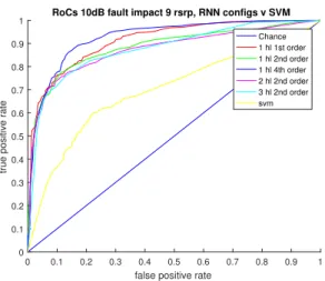
For a fault impact of 20dB (Fig 5), we can see that the SVM performance is now down to about 85% at 10% FPR.. The rNNs, on the other hand, can achieve detection results in excess of 90% TPR at 10% FPR. If the fault impact is reduced to 10dB, as shown in Fig 6, the rNNs can achieve a TPR in the region of 70% - 75% at FPR 10%,
0 0.1 0.2 0.3 0.4 0.5 0.6 0.7 0.8 0.9 1 false positive rate
0 0.1 0.2 0.3 0.4 0.5 0.6 0.7 0.8 0.9 1 tru e po si tive ra te
RoCs 20dB fault impact 9 rsrp, RNN configs v SVM Chance 1 hl 1st order 1 hl 2nd order 1 hl 4th order 2 hl 2nd order 3 hl 2nd order svm
Fig. 5. RNN and SVM Results for fault impact 20dB
which is a significant improvement on the equivalent SVM performance. From this work we found that in this specific scenario there is insignificant advantage in utilising the more complex configurations, but the single layer with second order filtering generally performs better than the simplest single layer configuration with no additional filtering. Hence we recommend the use of the single layer second order filtering approach for this scenario, providing a highly efficient run time detection capability which could therefore be deployed in the RAN on a devolved basis with minimal requirements for additional computing power.
0 0.1 0.2 0.3 0.4 0.5 0.6 0.7 0.8 0.9 1 false positive rate
0 0.1 0.2 0.3 0.4 0.5 0.6 0.7 0.8 0.9 1 tru e po si tive ra te
RoCs 10dB fault impact 9 rsrp, RNN configs v SVM Chance 1 hl 1st order 1 hl 2nd order 1 hl 4th order 2 hl 2nd order 3 hl 2nd order svm
Fig. 6. RNN and SVM Results for fault impact 10dB
VII. CONCLUSION
In this work we apply deep learning techniques to the cell coverage degradation detection problem. We show that the rNN technique can provide greater detection sensitivity than the best of current approaches, represented by the SVM technique, while at the same time eliminating the need for a separate hand coded data dimensionality reduction stage. We show that by using nine RSRP input channels this improve-ment in detection sensitivity can be achieved by using an rNN with a single hidden layer, minimising the need for run time computing power.
REFERENCES
[1] H. Ishii, Y. Kishiyama, and H. Takahashi, “A novel architecture for lte-b: C-plane/u-plane split and phantom cell concept,” in Globecom
Workshops (GC Wkshps), 2012 IEEE. IEEE, 2012, pp. 624–630.
[2] T. Nakamura, S. Nagata, A. Benjebbour, Y. Kishiyama, T. Hai, S. Xi-aodong, Y. Ning, and L. Nan, “Trends in small cell enhancements in lte advanced,”Communications Magazine, IEEE, vol. 51, no. 2, pp. 98–105, 2013.
[3] A. Mohamed, O. Onireti, M. A. Imran, A. Imran, and R. Tafazolli, “Control-data separation architecture for cellular radio access networks: A survey and outlook,” IEEE Communications Surveys & Tutorials, vol. 18, no. 1, pp. 446–465, 2016.
[4] J. Lee, Y. Kim, H. Lee, B. L. Ng, D. Mazzarese, J. Liu, W. Xiao, and Y. Zhou, “Coordinated multipoint transmission and reception in lte-advanced systems,”Communications Magazine, IEEE, vol. 50, no. 11, pp. 44–50, 2012.
[5] J. G. Andrews, S. Buzzi, W. Choi, S. V. Hanly, A. Lozano, A. C. K. Soong, and J. C. Zhang, “What will 5g be?”IEEE Journal on Selected
Areas in Communications, vol. 32, no. 6, pp. 1065–1082, Jun. 2014.
[6] R. Zhao, R. Yan, Z. Chen, K. Mao, P. Wang, and R. X. Gao, “Deep learning and its applications to machine health monitoring: A survey,”
arXiv preprint arXiv:1612.07640, 2016.
[7] G. F. Ciocarlie, C. Connolly, C.-C. Cheng, U. Lindqvist, S. Nov´aczki, H. Sanneck, and M. Naseer-ul Islam, “Anomaly detection and diagnosis for automatic radio network verification,” inInternational Conference
on Mobile Networks and Management. Springer, 2014, pp. 163–176.
[8] G. F. Ciocarlie, U. Lindqvist, S. Nov´aczki, and H. Sanneck, “Detecting anomalies in cellular networks using an ensemble method,” inNetwork
and service management (CNSM), 2013 9th international conference on.
IEEE, 2013, pp. 171–174.
[9] A. Zoha, A. Saeed, A. Imran, M. A. Imran, and A. Abu-Dayya, “Data-driven analytics for automated cell outage detection in self-organizing networks,” in Design of Reliable Communication Networks (DRCN),
2015 11th International Conference on the, Mar. 2015, pp. 203–210.
[10] W. Xue, M. Peng, Y. Ma, and H. Zhang, “Classification-based ap-proach for cell outage detection in self-healing heterogeneous networks,”
in 2014 IEEE Wireless Communications and Networking Conference
(WCNC). IEEE, 2014, pp. 2822–2826.
[11] J. Wang, N. Q. Phan, Z. Pan, N. Liu, X. You, and T. Deng, “An improved tcm-based approach for cell outage detection for self-healing in lte hetnets,” inVehicular Technology Conference (VTC Spring), 2016
IEEE 83rd. IEEE, 2016, pp. 1–5.
[12] W. Xue, H. Zhang, Y. Li, D. Liang, and M. Peng, “Cell outage detection and compensation in two-tier heterogeneous networks,” International
Journal of Antennas and Propagation, vol. 2014, 2014.
[13] O. Onireti, A. Zoha, J. Moysen, A. Imran, L. Giupponi, M. Imran, and A. Abu Dayya, “A cell outage management framework for dense heterogeneous networks,”IEEE Transactions on Vehicular Technology, vol. PP, no. 99, p. 1, 2015.
[14] F. Chernogorov, S. Chernov, K. Brigatti, and T. Ristaniemi, “Sequence-based detection of sleeping cell failures in mobile networks,” Wireless Networks, p. 1, Oct. 2015. [Online]. Available: http://dx.doi.org/10.1007/s11276-015-1087-9
[15] F. Chernogorov, I. Repo, V. R¨ais¨anen, T. Nihtil¨a, and J. Kurjenniemi, “Cognitive self-healing system for future mobile networks,” inProc. Int.
Wireless Communications and Mobile Computing Conf. (IWCMC), Aug.
2015, pp. 628–633.
[16] Y. Zhang, N. Liu, Z. Pan, T. Deng, and X. You, “A fault detection model for mobile communication systems based on linear prediction,”
in Communications in China (ICCC), 2014 IEEE/CIC International
Conference on. IEEE, 2014, pp. 703–708.
[17] W. Sun, R. Zhao, R. Yan, S. Shao, and X. Chen, “Convolutional discriminative feature learning for induction motor fault diagnosis,”
IEEE Transactions on Industrial Informatics, 2017.
[18] L. Jing, T. Wang, M. Zhao, and P. Wang, “An adaptive multi-sensor data fusion method based on deep convolutional neural networks for fault diagnosis of planetary gearbox,” Sensors, vol. 17, no. 2, p. 414, 2017.
[19] R. Zhao, R. Yan, J. Wang, and K. Mao, “Learning to monitor machine health with convolutional bi-directional lstm networks,”Sensors, vol. 17, no. 2, p. 273, 2017.
[20] B. Y. Goodfellow, I. and A. Courville,Deep Learning. MIT Press, 2016.
[21] 3GPP TR 36.873, “3rd generation partnership project; technical speci-fication group radio access network; study on 3d channel model for lte (release 12),” 2015-06, v12.2.0.