AFIT Scholar
AFIT Scholar
Faculty Publications 8-6-2018Cyber Anomaly Detection: Using Tabulated Vectors and
Cyber Anomaly Detection: Using Tabulated Vectors and
Embedded Analytics for Efficient Data Mining
Embedded Analytics for Efficient Data Mining
Robert J. GutierrezKenneth W. Bauer
Air Force Institute of Technology Bradley C. Boehmke
Cade M. Saie United States Army Trevor J. Bihl
Air Force Research Laboratory
Follow this and additional works at: https://scholar.afit.edu/facpub
Part of the Theory and Algorithms Commons
Recommended Citation Recommended Citation
Gutierrez, Robert J.; Bauer, Kenneth W.; Boehmke, Bradley C.; Saie, Cade M.; and Bihl, Trevor J., "Cyber Anomaly Detection: Using Tabulated Vectors and Embedded Analytics for Efficient Data Mining" (2018). Faculty Publications. 60.
https://scholar.afit.edu/facpub/60
This Article is brought to you for free and open access by AFIT Scholar. It has been accepted for inclusion in Faculty Publications by an authorized administrator of AFIT Scholar. For more information, please contact [email protected].
Cyber anomaly detection: Using
tabulated vectors and embedded
analytics for efficient data mining
Robert J Gutierrez
1, Kenneth W Bauer
1,
Bradley C Boehmke
1, Cade M Saie
2and Trevor J Bihl
3Abstract
Firewalls, especially at large organizations, process high velocity internet traffic and flag suspicious events and activities. Flagged events can be benign, such as misconfigured routers, or malignant, such as a hacker trying to gain access to a specific computer. Confounding this is that flagged events are not always obvious in their danger and the high velocity nature of the problem. Current work in firewall log analysis is manual intensive and involves manpower hours to find events to investigate. This is predominantly achieved by manually sorting firewall and intrusion detection/prevention system log data. This work aims to improve the ability of analysts to find events for cyber forensics analysis. A tabulated vector approach is proposed to create meaningful state vectors from time-oriented blocks. Multivariate and graphical analysis is then used to analyze state vectors in human–machine collaborative interface. Statistical tools, such as the Mahalanobis distance, factor analysis, and histogram matrices, are employed for outlier detection. This research also introduces the breakdown distance heuristic as a decomposition of the Mahalanobis distance, by indicating which variables contributed most to its value. This work further explores the application of the tabulated vector approach methodology on collected firewall logs. Lastly, the analytic methodologies employed are integrated into embedded analytic tools so that cyber analysts on the front-line can efficiently deploy the anomaly detection capabilities.
Keywords
Anomaly detection, digital forensics, Mahalanobis distance, tabulated vectors
Received 26 March 2017; Revised received 31 January 2018; accepted 26 March 2018
Introduction
Due to the constantly changing behavior of cyber-attacks, reactive approaches are desirable to detect and prevent malicious actors from gaining access to networks. Firewalls and intrusion detection and pre-vention systems (IDPS) are a line of defense in identi-fying and stopping suspicious internet traffic. When a suspicious event occurs, these devices generate a log file containing details of what preprogrammed rules were violated and how it was handled.1Such log files contain details of the event, e.g. source and destination IP addresses, port numbers, and protocols, but not the packet and data that led to the event. Of interest is cyber/digital forensics of logged events to understand their origin and magnitude.2,3Suspicious events include both malicious and non-malicious activities, e.g. mis-configured routers; however, each event is logged and
to find malicious events for further analysis, one must search through all logged suspicious events.
Although advances have been made in applying text mining and advanced analytics to cyber log data analysis, c.f. Suh-Lee et al.4 Breier and Branisova´5 and Villa et al.,6the characteristics of cyber logs results in much manual analysis for interpretation and response.7–10When considering log data, cyber analysts
1
Air Force Institute of Technology, Dayton, OH, USA 2
U.S. Army, Lorton, VA, USA 3
Air Force Research Laboratory Sensors Directorate, Wright-Patterson AFB, OH, USA
Corresponding author:
Bradley C Boehmke, Air Force Institute of Technology, 2950 Hobson Way, Dayton, OH 45415, USA.
Email: [email protected]
Journal of Algorithms & Computational Technology 2018, Vol. 12(4) 293–310
!The Author(s) 2018 Article reuse guidelines: sagepub.com/journals-permissions DOI: 10.1177/1748301818791503 journals.sagepub.com/home/act
Creative Commons Non Commercial CC BY-NC: This article is distributed under the terms of the Creative Commons Attribution-NonCommercial 4.0 License (http://www.creativecommons.org/licenses/by-nc/4.0/) which permits non-commercial use, reproduction and distribution of the work without further permission provided the original work is attributed as specified on the SAGE and Open Access pages (https://us. sagepub.com/en-us/nam/open-access-at-sage).
rely on manual sorting and experiential knowledge to find possible threats in logged events to further inves-tigate.7,11,12Thus, cyber security is heavily experiential-based and uses the innate ability of humans to process large amounts of complex data;13 similarly experience is critical and novice analysts might miss intrusions and events that a veteran analyst would not.14Additionally, cyber intrusion detection is asymmetrical in nature whereby an attacker can focus on only one threat approach while a defender (cyber analyst) must con-stantly protect all systems and prepare for many differ-ent types of attacks, vulnerabilities and threats.15 Although system administrators and cyber analysts manually handle log data, this is becoming increasingly infeasible due to the big data nature of cyber traffic (unstructured, high volume and high velocity16).
Normal behavior for cyber networks is generally not well defined and changes over time, resulting in high false positive detection rates.17Additionally, since fire-wall log events are the result of network abnormalities, one is thus necessarily interested in detecting the anom-alies within the anomanom-alies. Related research, c.f. Lazarevic et al.,18Denning,19Garcıa-Teodoro et al.,20 Grimaila et al.,21 Moore et al.,22 Dube et al.,23 Shilland,24 Shen et al.,25 Stewart et al.26 has focused on anomaly detection at the device/software level, with little21,27–32 exploration into anomaly detection in the log files generated from the preexisting devices or software.
For analysis, data were used from a large scale dis-tributed network with regional data nodes much like the Microsoft Cyber Defense Center, the Verizon Network Operations Center, or AT&T Global Network Operations Center. Currently, data is
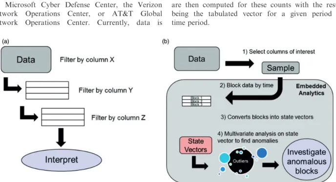
analyzed from enterprise-wide networks, which rely on a series of firewalls and IDPS to identify and stop intrusions. These devices, when triggered, generate a log file containing details of how it handled each inci-dent, such as the source and destination IP addresses, port numbers, protocols, bytes transferred, etc. However, due to the wide variety of devices adding observations to the log, the data can be highly variable. In operation, analysts employ an experiential approach whereby large log files are manually sorted to find anomalies to further investigate; this process is concep-tualized in Figure 1(a). However, due to the large size of the network and quantity of users, the data is of significant volume and emerging at high velocity; thus representative of a big data problem. Currently, ana-lysts inspect numerous potential incidents on a daily basis, but have neither the time nor the resources avail-able to analyze all incidents contained in the logs.
This paper combines statistical and visual methods and integrates them into embedded analytic applications to assist analysts in the manual analysis of firewall logs. To this end, the authors devel-op a tabulated vector approach (TVA) that processes firewall log files to identify anomalies within the flagged firewall log event data. The TVA process employed by the authors is similar to that of Winding et al.,27wherein pre-defined data attributes are consid-ered. The developed process is automated and data attributes are transformed into representative counts, e.g. the number of times a certain IP address appears within the timespan of interest. Descriptive statistics are then computed for these counts with the result being the tabulated vector for a given period of time period.
Figure 1. Cyber firewall log analysis methods: (a) Standard, manual intensive, cyber anomaly detection approach; (b) proposed
The authors propose an analyst-aided solution to cue system administrators and analysts to anomalies for further analysis when manual log file analysis and forensics are employed. The end goal is that seen in Figure 1(b), wherein log files are selected, these are then divided into time blocks. From here, tabulated vectors are computed for the time blocks. These tabu-lated vectors are then processed through statistical and graphical methods. Finally, analysts are cued to various blocks of interest within a given log data file. The purpose of this approach is to efficiently analyze abnormal activities so that cyber analysts can dedicate their time to researching potential threats.
This paper is organized as follows: “Background” section reviews background details on cyber networks, cyber threats, and cyber technologies. “Developing a sta-tistical framework for cyber anomaly detection” section 3 presents statistical pattern recognition methods that consider handling unstructured data through numerical approaches. “TVA for firewall log analysis” section dis-cusses the development of a framework to detect firewall log anomalies. “Embedded analytics” section discusses how the proposed methodology was embedded into ana-lytic applications for use by cyber analysts, and “Conclusions” section concludes the paper.
Background
In order to analyze cyber log data, one must discuss the basics of cyber networks, firewalls, IDPS, and charac-teristics of cyber log data. In this paper, we will discuss the salient characteristics of these areas.
Cyber networks
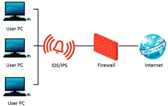
Figure 2 presents a conceptualization of a basic cyber network where user PCs are protected by an intrusion detection system (IDS) or intrusion prevention system (IPS), collectively IDPS, and a firewall.33Each security device plays a crucial role in protecting the user’s com-puter from outside and inside threats. Both IDPS and firewalls monitor network traffic and either stop or flag events that violate their rules. When an event triggers a rule, details are logged along with the action taken by the firewall or IDPS.
Firewalls. Firewalls provide a first level of protection between an internal (e.g. local area network (LAN)) and external (e.g. internet) network. Firewalls employ rules to determine the outcome of an event34 and pre-vent risks, including: (1) an internal host system’s expo-sure to inherently insecure Internet protocols and services, and (2) probes and attacks launched from hosts on the Internet.35 A wide variety of firewalls exist, including both commercially developed and open source systems.36 Presently, firewalls employed in the operational network of interest include those manufactured by Palo Alto Networks, Cisco ASA, McAfee, and Norton 360.
Firewalls are of three general types:35(1) packet fil-tering (PF), (2) proxy gateway, and (3) circuit level inspection. In brief, PF firewalls consider each incom-ing and outgoincom-ing packet, apply predefined rules to ana-lyze the packet and decide to allow it to proceed or not.35 Proxy gateways, also known as servers, act as a security filter.35 Circuit level inspection firewalls
use a proxy server that employs an access control list to determine if a request is permitted.
Intrusion detection/prevention systems (IDPS)
Intrusion detection involves monitoring and logging network traffic to detect attempts to gain unauthorized network access which are evident by security policy violations and acceptable use policy.37 Intrusion pre-vention goes one step further by attempting to stop such incidents. Therefore, IDPS must identify possible incidents and when one occurs, a log of information about the event and the course of action is generated.37 Similar to firewalls, IDPS employs a set of rules related to signatures or anomalies.37 IDPSs can be setup in two ways, host based (HIDS) or network based (NIDS), where the former is deployed on each individ-ual computer while the latter is positioned along the network.37
Cyber anomaly detection in firewall logs
While one could find that a given firewall log file con-tains entirely malicious events, one likely has the prob-lem of too many false positives in the log data. False positive issues in cyber anomaly detection involve too many benign events being logged and thus obscuring the rare malicious activities.38 Since firewall logs con-tain anomalous events detected within network traffic and since many of these are not threats from attackers, one is thus interested in finding anomalies among anomalies. Two general paradigms exist for this task: (i) experiential, or manually searching through logs based on subjective experiences and (ii) statistical or machine learning approaches to find observations of interest in the log data.
Experiential approaches
In general, the work of cyber analysts is manual inten-sive and involves queries and searches of a dataset.7,11 Experiential approaches work by taking a log files, employing various sorting and analysis tools (e.g. Snort and Kibana), and incorporating contextual information to understand an event.11 The process is conceptualized in Figure 1(a), where only two column searches are considered, which illustrates the manual nature of sorting by individual columns until one finds observations that display suspicious behavior. While such an approach could be highly accurate, it is time consuming and requires a year or more of on the job experience11 and learning of various firewall forensics attributes.39
Statistical data analysis
Statistical data analysis involves using mathematical approaches to find patterns in datasets.13,40 Approaches for doing so range from supervised (known classes/groups in the data) to unsupervised (unknown classes/groups in the data). Statistical data analysis thus includes classification methods where classes are known, at least in the training data, to clus-tering methods for which classes are unknown and one aims to find groupings in the data.13In cyber analysis, one can divide the field into academic and operational approaches. While academic approaches to cyber anal-ysis frequently have the luxury of knowing if behaviors are threats or not, c.f. Grimaila et al.,21Moore et al.,22 operational cyber analysis does not have the luxury of canonical truth. Thus, statistical analysis of cyber data is frequently unsupervised in operation.
Since a variety of methods have been proposed to analyze firewall logs via statistical or machine learning methods, of interest is thus leveraging past concepts and ideas to create a method to aid analysts in analyz-ing and interpretanalyz-ing firewall log data. A variety of approaches exist in this domain, c.f. Lazarevic et al.,18Garcıa-Teodoro et al.,20and include text ana-lytics,41 support vector machines,18 random forests,42 event correlation,21,30,43–46 dynamic rule creation,29 and principal component analysis.20,47,48Of particular interest is the work of Denning,49 who originally proposed using anomaly detection methods in cyber security. This has been consistently extended and expanded upon, as seen in Lazarevic et al.,18 Garc ıa-Teodoro et al.,20Zhang and Zulkernine,42Shyu et al.,47 Wang and Battiti,48Lazarevic et al.,50 Ahmed et al.,51 Liao et al.,1and Patcha and Park.52
Cyber network and data of interest
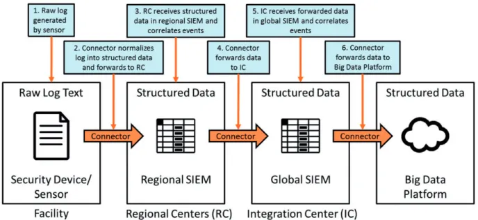
Of interest to the authors are general firewall log files, one task is handling all firewall logs from the many networks the enterprise has worldwide. For context, the operational approach to the data collection process is conceptualized in Figure 3. For data handling, raw logs are first normalized into a structured data file by a connector, a stand-alone device or software that for-wards data and sometimes converts from one format to another. These are then forwarded to regional centers (RC). RCs are organizations that provide regional services while simultaneously defending the network from cyber threats.53 At the RCs, a regional security information and event management (SIEM) device aggregates, correlates, monitors, and generates alerts from the received data. Next, a second connector for-wards the data to a global SIEM known as the integra-tion center (IC). After the data is reprocessed at the IC,
it is then uploaded into a big data platform—a central-ized database for managing big data,7both structured and unstructured, at high volume and high velocity.16 From here, data can be queried and analyzed.
Developing a statistical framework
for cyber anomaly detection
In order to develop a statistical framework for firewall log analysis, the authors posit that a multivariate data-set containing only numeric values is necessary. To this aim, the authors work towards feature vector creation and then statistical and graphical analysis of this fea-ture vector.
Feature vector creation
One technique to facilitate the application of statistical methods to log files is the feature vector method pro-posed by Winding et al.,27and further applied in Breier and Branisova29 Syurahbil et al.54 This approach aggregates log file observations into a set of feature vectors, which can then be analyzed through statistical approaches, which require the data to be numeric. In brief, a feature vector is a count of occurrences for the unique values in a set of variables.27 Inherently, this involves dividing the data into blocks or regions of sequential observations.
A conceptualization is presented in Figure 4. In Figure 4(a), we have an example of two columns of raw data in a given block. Field A is categorical and field B is numeric. A feature vector can be created by condensing these observations into a block row,
Figure 4(b). Unique categorical features in field A become columns of block 1. The count of each unique categorical feature in that block then becomes the value. Numerical entries in field B the original data are then summed with that value placed in the column for B.
When applying the feature vector approach to fire-wall log data, Winding et al.,27 took log file records with the following raw data fields:
• Repeated attempts of access by a single IP,
• Number of source IPs per destination IP,
• Number of destination IPs per source IP,
• Number of destination ports on a given source/ destination IP pair,
• Unique IPs,
• Maximum activity from a single IP,
• Failed and successful connections from the same IP,
• Attempts to access invalid IPs,
• Inbound/Outbound bytes per unit time.
and then condensed these into feature vectors with the following variables:
• Source IP address, number of destination IP addresses,
• Destination IP, number of failed access attempts,
• Source IP, destination IP,
• Destination perspective vector (destination IP, count of source IPs, number of successful accesses, number of failed accesses, count of destination ports, number of bytes transferred (inbound), number of bytes transferred (outbound)).
Mahalanobis based anomaly detection
To find anomalies inside a feature vector, one approach is the Mahalanobis distance, which is a multivariate outlier detection expression, which compares each observation by its distance from the data mean, inde-pendent of scale.55 The Mahalanobis distance is com-puted as
MD¼pffiffiffiffiffiffiffiffiffiffiffiffiffiffiffiffiffiffiffiffiffiffiffiffiffiffiffiffiffiffiffiffiffiffiffiffiffiffiffiðxxÞC1ðxxÞ (1)
wherexis a vector ofpobservations,x¼ðx1;. . .;xpÞ,
x is the mean vector of the data,x¼ðx1;. . .;xpÞ, and
C1 is the inverse data covariance matrix.55 Once computed, MD values can be sorted with anomalies identified by relative magnitudes.
Breakdown distance
However, one limitation is usingMDis that it does not provide a rationale for what is or is not an anomaly. Therefore, we propose the use of a “breakdown dis-tance” (BD) BDi¼ ðxixiÞ ffiffiffiffiffiffi Cii p (2)
wherexiis a given variable,xi is the mean of the
var-iable, and Cii is the variance of xi. The advantage of
equation (2) is that scaling by variance enables one to measure of the relative contribution of each variable to MDscores.
Principal components and factor analysis
Principal components analysis (PCA) is a linear trans-formation method which involves computing the data covariance, or correlation, matrix eigen-solution pro-jecting the data by these eigenvectors.56 The resultant projection is of uncorrelated components, with each component explaining successively less variation in the data, per the eigenvalues.56PCA is a dimensionality reduction method because one can select a small amount of components which explain a large amount of the variance in the data. PCA was applied to IDPS event analysis by Garcia-Teodoro et al.;20Shyu et al.,47 proposed using minor components (those whose vari-ance explained is less than 0.20), claiming that their method can distinguish whether an outlier is an extreme value or it does not have the same correlation structure as the “normal” data.
Similar to PCA, factor analysis (FA) is another dimensionality reduction technique designed to identify underlying structure of the data. FA relates the corre-lations between variables through a set of factors to link together seemingly unrelated variables.56,57 An additional step seen in FA is that it can rotate the original solution seen in PCA, in order to possibly find more structure in the data. The basic FA model is
X¼Kfþe (3)
where X is the vector of responses X¼ðx1;. . .;xpÞ, f
are the common factorsf¼ f1;. . .;fq
,eis the unique factors e¼ðe1;. . .;epÞ, andKis the factor loadings.56
For the desired results, this research uses the correla-tion matrix. Factor loadings are correlacorrela-tions between the factors and the original data and can thus range from 1 to 1, which indicate how much that factor affects each variable.56 Values close to 0 imply a weak effect on the variable.
A factor loading matrix can be computed to under-stand how each original data variable is related to the resultant factors.56This can be computed as
K¼ ffiffiffiffiffiffiffiffiffiffiffiffiffiffiffiffiffiffiffiffiffiffiffiffiffiffiffiffiffiffiffiffiffiffiffiffiffik1e1;. . .;pffiffiffiffiffiffiffiffiffiffiffikpep
q
(4)
wherekiis the eigenvalue for each factor, eiis the
eigen-vector for each factor, and p is the number of col-umns.56 Factor scores are used to examine the behavior of the observations relative to each factor. This research will plot factor scores against one anoth-er as a method for anomaly detection. Using equation (4), the scores are calculated as
b
f ¼ XsR1K (5)
where Xs is the standardized observations, R1 is the
inverse of the correlation matrix, and K is the factor loadings matrix.56To simplify the results for interpre-tation, the factor loadings can undergo an orthogonal or oblique rotation.58 Orthogonal rotations assume independence between the factors while oblique rota-tions allow the factors to correlate. For this research, we utilize the most common rotation option known as varimax.59Varimax rotates the factors orthogonally to maximize the variance of the squared factor loadings which forces large factors to increase and small ones to decrease, providing easier interpretation.
To assess the quality of a factor analysis solution, Kaiser60 proposed the index of factorial simplicity (IFS) that measures the tendency towards unifactorial-ity for both a given row and the entire matrix as a whole. Computing IFS values consistent with Kaiser,60we can evaluate the quality for a factor anal-ysis solution with the heuristic labels shown in Table 1. Since the purpose of factor analysis is for dataset reduction, we consider the three generally accepted methods of determining the dimensionality for correla-tion matrix inputs.56,61 The first and most commonly used is Kaiser’s Criterion62 which advises to retain those factors whose eigenvalues are greater than 1.0. Second is Cattell’s scree test63which involves graphing the eigenvalues and retaining those that form the steep curve. The third method is a modified scree test called Horn’s parallel analysis (i.e. Horn’s Curve),64that uses a Monte Carlo simulation to find the average eigenval-ues. Due to the advantages of Horn’s parallel analysis,
the authors employed this method herein to determine the number of factors to explore.
Visualizations
Graphical analytic tools enable an analyst to visualize insights that may not be readily apparent without man-ually examining the data.65Appropriate visualizations are key to cyber data analysis, c.f. Schweitzer and Fulton,66thus the authors present a selection of meth-ods which will be employed to help analysts tell a story in firewall log data.
Heatmaps
Heatmaps are graphical representations of a data matrix through the use of a color scale and have been used for 100þyears as an effective visualization approach for a matrix.67In statistics, one common use for heatmaps is for correlation matrices, illustrating the relationship between variables ranging from1 to 1.
Histogram matrix
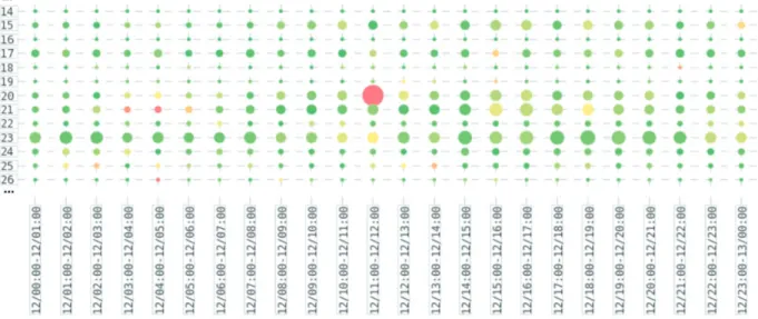
A histogram matrix (HMAT) is a visualization tech-nique developed by Frei and Rennhard,28 that com-bines graphical and statistical techniques to aid security administrators in efficiently identifying anom-alies. HMAT was designed to scan large log files that show steady normal behavior and examine the mes-sages displayed for each observation. HMAT extends both heatmaps and histograms, where data values are represented through a series of circles on a grid with the radius directly corresponding to the magnitude.28
An example HMAT relative to log files is presented in Figure 5 (taken from Frei and Rennhard28); here HMAT visualizes time on the x-axis, and the number of words per message on the y-axis. The size of the circle in Figure 5 is related to the number of log mes-sages with the corresponding number of words while the color serves as indication to the relative likelihood of the time slot. The authors in Frei and Rennhard28 determined the color of a circle by comparing the dis-tribution of the sizes of the circles in its column with previous columns. In Figure 5, the large red circle
Table 1. Kaiser’s evaluation of the IFS levels.61
IFS level Evaluation
In the 0.90s Marvelous In the 0.80s Meritorious In the 0.70s Middling In the 0.60s Mediocre In the 0.50s Miserable Below 0.50 Unacceptable
indicates an unusually large amount of messages, great-er than 5 standard deviations from the norm. HMAT also provides user interaction, where an administrator can click on one of the circles to reveal all the log messages that define that circle.
Network graphs
Network graphs are graphical models that depict a relationship between two or more nodes, connected by edges.68,69 Herein, the authors employ network graphs to illustrate the interaction between source and destination IP addresses. Of particular interest are identifying The Onion Router (TOR) related IP addresses, port scans, and network fingerprinting attempts. TOR is a network of servers that provides a user with anonymity by relaying their internet traffic through multiple encrypted servers.70,71Probable TOR nodes can be found and might be related to attempts to access multiple computers. A port scan is the act of determining which ports on a network are open and is thus related with one source IP connecting to many destination IPs over a short amount of time.72,73 Finally, fingerprinting a network is the act of revealing the presence of cyber security devices.73 Thus, each unique IP address is a node. An edge represents the interaction between sources and destinations with its thickness denoting the frequency of interactions between the nodes. For related work, see Swanson.74
TVA for firewall log analysis
Assembling the statistical methods from “Developing a statistical framework for cyber anomaly detection” sec-tion together involves a systems engineering approach. Here, the authors will show how the statistical methods
from “Developing a statistical framework for cyber anomaly detection” section can be assembled into a cohesive firewall log analysis framework. Then the authors will illustrate the utility of their framework with an example case study.
TVA approach and process
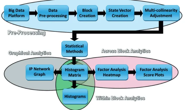
When incorporating the statistical, graphical, and ana-lytical methods discussed in “Developing a statistical framework for cyber anomaly detection” section, the conceptualization that appeared in Figure 1(b) yields the flow chart seen in Figure 6. Figure 6 presents a representation of the methodology used operationally to exploit log data is presented. This process in Figure 6 is broken up into four subsections: pre-processing, within block analytics, across block analytics, and graphical analytics. Pre-processing takes the raw data and transforms it into a form that can be used for sta-tistical analysis. Stasta-tistical analysis utilizes the statisti-cal tools described in “Developing a statististatisti-cal framework for cyber anomaly detection” section to build the HMAT for anomaly detection. Moving to within block analytics, histograms are utilized to com-pare the data between blocks in time. Across block analytics assesses the entire dataset for similarities or differences while graphical analytics focuses on deter-mining the link between observations and IP addresses. Developing a data analysis platform also involved sys-tems engineering to select and incorporate available packages and tools for functionality. R75 was used due to its growing popularity and open source nature;76additionally, R is further available as a soft-ware tool for big data platforms.
TVA example case study
To illustrate the utility of the proposed firewall log anomaly detection process, the authors will examine a representative log file with 39,304 observations and 400þdata features. Due to the nature of the data sour-ces, IP address and data fields have been obfuscated to permit the presentation of real data results. Thus, IP addresses will not be in the traditional XXX.XXX.XX. XXX format, obfuscated values will appear in figures and nondescript names (e.g., 239e330c.4c3e44ed. f54890e4.1a9d80ce) will appear in the text. Additionally, data fields will be vague and generic.
Data pre-processing
Once data is retrieved, the data must be pre-processed and then time regional blocks are created, from which state vectors are extracted and data quality is consid-ered (e.g. multicollinearity adjustments). These steps are necessary to incorporate multivariate and graphical methods for anomaly detection. In this step, variables of interest are either selected or created to aid in the discovery of anomalies.
The data used in this research has been collected from sensors located around the world. While over 400 data fields are collected, for illustrated purposes this research focuses on the fields shown in Table 2. These fields were selected based on (i) commonality between multiple log files and (ii) their ease on
demonstrating the proposed methodology without the use of text mining techniques. Since some device ven-dors can have multiple products, we combine the fields Device_VendorandDevice_Productto form a new var-iable Device_Name to avoid confusion between the device the observation originated from.
Time block creation
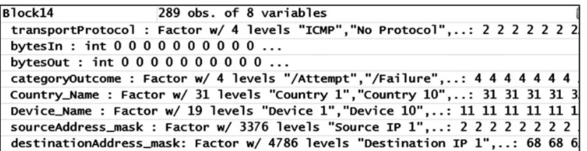
Following pre-processing and data cleaning, one then creates time regional blocks. Here, the observations are divided into sequential time blocks of equal length. The 39,304 observations in the example log file were chro-nologically separated into 136 time blocks, each con-taining 289 observations. Figure 7 shows the categorical variables being labeled as factors while
Figure 6. Multivariate and graphical approach to firewall log anomaly detection.
Table 2. Dataset variables.
Field name Description
Device Vendor Company who made the device
Device Product Name of the security device
Source Address IP address of the source
Destination Address IP address of the destination
Transport Protocol Transport protocol used
Bytes In Number of bytes transferred in
Bytes Out Number of bytes transferred out
Category Outcome Action taken by the device
numerical variables being labeled as numeric (integer, double, long, etc.). The number of levels associated with a categorical variable then denote the number of unique entries. For example, theDevice_Namevariable has 19 levels in the example log file, indicating that there are 19 different devices found in this dataset.
State vector creation
From the time blocks, numerical matrices are extracted to prepare for statistical analysis. To apply the statisti-cal methods discussed in “Developing a statististatisti-cal framework for cyber anomaly detection” section, we employ TVA, which uses the feature vector creation method of “Feature vector creation” section to take the pre-defined data attributes and transform them into representative counts using descriptive statistics. Therefore, as each time block is generated, the categor-ical fields are separated by their levels and a count of occurrences for each level is recorded into a vector. All numerical fields, such as bytes in and bytes out, are recorded as a summation within the time block. Due to the large number of levels associated with IP addresses, only the top 10 source and destination IP address counts are recorded. These vectors are then aggregated into a single matrix, known as the state vector matrix, as seen in Table 3. In Table 3, one sees rows for time blocks 1–5 with a count of occurrences for each device found in the data.
Multicollinearity adjustment
Prior to any statistical analysis, we automatically inspect the state vector for multicollinearity issues.
This prevents us from inadvertently having issues such as matrix singularity, rank deficiency, and strong correlation values; this also removes any columns that pose an issue. The conclusion of this step ensures the data is ready for statistical analysis.
Before the statistical tools, mentioned in “Developing a statistical framework for cyber anomaly detection” section, are applied to the state vector matrix, the columns of the state vector matrix must meet three criteria: (1) the columns must have a vari-ance greater than 0þD1 to avoid matrix singularity,
whereD10.1; (2) the columns must be linearly
inde-pendent to avoid computational errors associated with rank deficiency, consistent with;60(3) the values of the correlation matrix cannot exceed a threshold of 1D2,
where D2¼0.05. The identified columns are removed
and the reduced state vector matrix is ready for multi-variate analysis.
Statistical analysis
Once the data has been pre-processed and made to conform to general data quality expectations, our data is ready for analysis. First we can build the HMAT to serve as the foundation to subsequent anal-ysis. From here, the further analysis is analyst driven whereby three directions can be explored: within block analytics, across block analytics, and graphi-cal analytics.
The HMAT in this research utilizes the squared Mahalanobis distance as an outlier detection metric to determine the color of each time block in the HMAT. The breakdown distance enhances
Figure 7. Sample of time block creation.
Table 3. Example state vector matrix.
ICMP No protocol TCP UDP /Attempt /Failure /Success No outcome Country 1 Country 10 Country 11
1 1 254 22 12 17 67 82 123 0 0 0 2 0 264 16 9 41 38 106 104 0 0 0 3 0 247 16 26 0 41 75 173 0 0 1 4 0 267 12 10 74 25 114 76 0 0 0 5 0 236 14 12 33 22 70 164 0 0 0 ... ... ... ... ... ... ... ... ... ... ... ...
the HMAT by adjusting the size of the circles accord-ing to its normalized value for each variable. Figure 8 shows the HMAT for the entire dataset, where each row refers to a time block and each column represents a variable. Using the Mahalanobis distance, the anom-alous time blocks are distinguished by the darker shade of blue. Then, to determine the size of the circle, we normalize the breakdown distance for each column to distinguish which variables contributed most to the Mahalanobis distance value within each time block.
Thus, from Figure 8, we can observe the big picture of potentially concentrated anomalies. The rows that are shaded darker imply that they are anomalies rela-tive to their MD. Then the columns that have larger
circles indicate those variables that are driving the MD for that particular time block. Looking at Figure 8, we identify the clearest anomalies shown in the lighter blue with the largest circle as blocks 14, 27, 44, and 63. We also recognize instances where sequential rows appear in the top 20 time blocks, which suggests that the block size may be too small. Moving forward with our case study approach, we select block 14 for further investigation.
Statistical analysis: Within blocks analytics
Once a time block has been selected for analysis, we first explore within block analytics through the
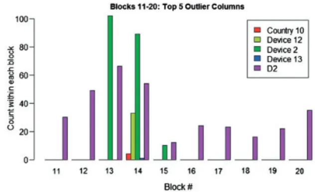
use of histograms, as seen in Figure 9. Here, we com-pare the counts of observations for particular attributes within neighboring time blocks. Once an anomalous time block is detected, histograms are generated to compare the state vector values relative to neighboring time blocks. The histogram shown in Figure 9 displays the frequency of occurrences for the top five columns with the largest BDvalue for block 14, relative to the occurrences for neighboring time blocks. The purpose is twofold: (1) observe the columns that cause the block to be an anomaly and (2) take note of the temporal relationship between the top five columns and the time blocks.
Based on Figure 9, we further our recommendation for a larger block size since blocks 13 and 14 both have high values for Device 2 and the D2 variable. The des-tination IP address labeled as D2 within block 14 is destination IPIPAddress1.
Statistical analysis: Across blocks analytics
The next direction we explore in statistical analysis is across block analytics. Using FA, we first explore the factor loadings (correlations between the columns of the state vector matrix and the suggested factors), then we compare the factor scores against one another for anomaly detection. To begin using factor analysis, the dimensions of the reduced state vector matrix are first passed to the Horn’s curve function to find the recommended set of eigenvalues. Next, the dimension-ality is determined by finding the eigenvalues of the correlation matrix of the state vector matrix and retain-ing only those factors whose eigenvalues are greater than or equal to those produced by Horn’s curve. The reduced state vector matrix and the number of factors to retain are passed to the factor analysis func-tion. Then, the factor analysis function generates two sets of factor scores and factor loadings, unrotated and rotated. Using the IFS values to assess the quality of our solutions, we select the set of scores and loadings associated with the larger IFS value. The factor
loadings are displayed in a correlation heatmap for interpretation of the variable relationships. The factor scores for each factor are plotted against one another for graphical anomaly detection.
After performing factor analysis, we observe the IFS levels presented in Table 2 to assess the quality of our factor analysis solutions. The rotated IFS level is higher than the original IFS level, serving as rationale for using the rotated factor loadings and scores in the subsequent analysis. According to Table 4, a value of 0.6125 is deemed as mediocre.
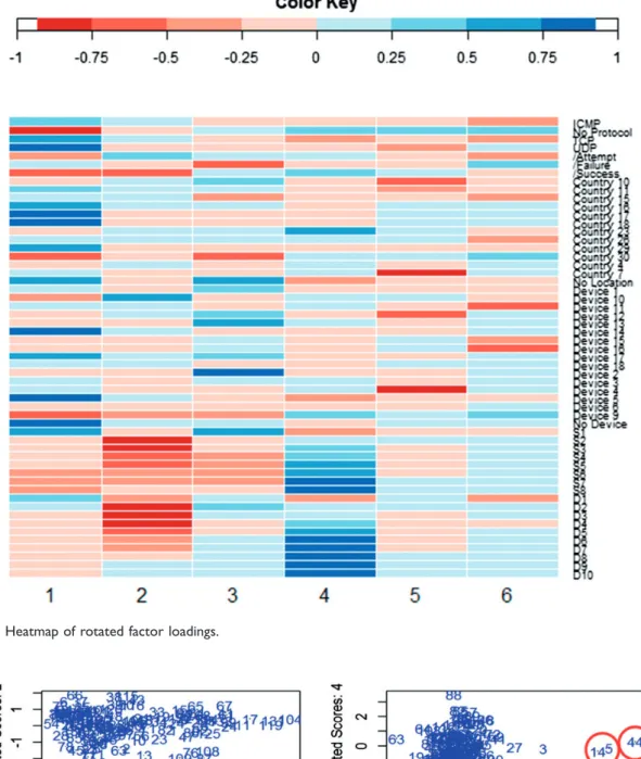
The heatmap in Figure 10 shows the correlation between the columns of the reduced state vector to the rotated factor loadings. Strong negative tions are depicted as red while strong positive correla-tions are shown as blue. The factor loading breakdown can provide insight into the relationships between var-iables based on Figure 10. For example, in factor 5 we see that the two devices, device 4 and device 13 are directly related to the geographic variables Country 7 and Country 10. While the true relationship between these variables is unknown, we may presume that these devices are set up to capture signatures from those locations. Looking at factor 1, we notice that four devi-ces as well as the two main protocols are highly corre-lated with observations coming from the geographic locations of Country 16, Country 17, Country 18, and Country 29. It is highly likely that these locations are associated with known TOR exit nodes. Interestingly, it also reinforces the relationship seen in the histogram in Figure 8, where observations sourced from Country 10 and detected by the Device 13 are correlated with high occurrences.
The next step of FA involves projecting the data by the factors. Figure 11 contains four subplots for this step: the subplot in the top left plots rotated scores 1 on the x-axis and rotated scored 2 on the y-axis; the sub-plot in the top right sub-plots rotated scores 3 on the x-axis and rotated scored 4 on the y-axis; the subplot in the bottom left plots rotated scores 5 on the x-axis and rotated scored 6 on the y-axis; the subplot in the bottom right plots rotated scores 3 on the x-axis and rotated scored 5 on the y-axis. Although rotated scores 1 explains the most variation in the data, followed by rotated scores 2 and so on, anomalies are not apparent until one examines rotated scores 3 and 5. Based on
Figure 9. Block 14: top 5 breakdown distance columns.
Table 4. IFS results.
IFS level Evaluation
Original 0.5674 Miserable
Rotated 0.6125 Mediocre
Figure 10. Heatmap of rotated factor loadings.
these plots, we can clearly see the anomalous time blocks, such as blocks 27, 63, 14, and 44.
Statistical analysis: Graphical analysis
The final analysis direction we examine is graphical analytics. This encompasses both the HMAT and the IP network graphs. The purpose of the network graphs is to visualize the connections between source IP addresses and the destination IP(s) they attempted to connect to. While not directly a statistical technique, this method allows for rapid visual cues to understand the IP dynamics within the dataset or a specific time block.
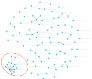
In Figure 12, we display the network graph for time block 14. At first glance, there is a noticeably large cluster on the bottom left (circled in red), where mul-tiple nodes are connected to a single node. We take a closer look at this region in Figure 13. Looking at Figure 1, we first pinpoint the source IP address asb7-fa0888.5aa3beb3.5aa3beb3.5aa3beb3. In the original data set, the source IP address could not be identified by the security device, either as a result of misconfigu-ration or the source masking their IP address. Next, we skim through the destination IP addresses con-nected to the focal source IP address. Coincidentally, we recognize the IP address 239e330c.4c3e44ed. f54890e4.1a9d80ce (denoted by a red dot), which was found to be the fifth highest variable causing time block 14 to be an anomaly. Then, we noticed a common trend, where seven other destination IP addresses began with 239e330c.4c3e44ed, three of which began with 239e330c.4c3e44ed.f54890e4. This suggests that the source IP address in this cluster was either attempt-ing to perform a port scan, or attemptattempt-ing to fattempt-ingerprint the network.
Embedded analytics
Analytic capabilities within organizations have, histor-ically, been dominated by proprietary software technol-ogies. Unfortunately, these technologies often lack availability, innovation, interoperability, flexibility, and transparency.77 Likewise, to incorporate the ana-lytic approach herein illustrated into existing proprie-tary software used by cyber analysts would take significant resources (i.e. time, money) of which most organizations have little to spare. In recent years, there has been an increased transition away from proprietary software and towards open source software both within the federal organizations and across industry. Open source software is a software that is voluntarily devel-oped and extended by users specific to their organiza-tion’s needs and made freely available to all.78 For analytic purposes, open source software allows analysts to customize analytic processes and products specific to their organization. Consequently, open source software has emerged as a major cultural and economic phe-nomenon79and illustrates the trend toward developing user innovation around analytic capabilities to increase an organization’s performance.80 This collaborative model offered by the open source ecosystem can poten-tially change the analytic nature of organizations by increasing innovation and technology adoption while being constrained by resources.81
The transition towards open source software allows us to operationalize and embed our analytic approaches into systems and business processes for more efficient analytic efforts.82 In this research, the authors developed two forms of embedded analytics: an open source R Package (anomalyDetection83) and a Shiny Application which is employed by cyber ana-lysts for operational analysis of log data.
Figure 12. Block 14 IP network graph.
anomalyDetection R Package
anomalyDetection is an R package that provides quan-titative cyber analysts the ability to effectively and effi-ciently implement our methodology. anomalyDetection provides 13 functions to aid in the detection of potential cyber anomalies. These functions employ the methods presented in this paper and described in Gutierrez et al.84
Shiny Application
Due to the high volume of incoming data, cyber ana-lysts may not always have the time available to manu-ally compute and analyze the data for anomaly detection using the anomalyDetection R package. To fully integrate the authors’ methodology into the work-flow of cyber analysts operating on a big data platform, a web-based embedded analytic was developed so the analysts can execute the analytic approach efficiently over multiple time periods and data sources. R Shiny was used to develop this second form of embedded analytic. Shiny is an R package that provides an ele-gant and powerful framework for building interactive web applications using R. The web application pro-vides means for the user to upload new data files, adjust block sizes and the number of IP addresses to consider. The web application will then perform the analytic methodologies discussed throughout this paper and provide results in the form of interactive
graphics and tables to help the cyber analyst detect anomalies. This provides an efficient approach for cyber analysts to effectively analyze significant amounts of data while ensuring the methodological approach is valid and consistent. Example screenshots of the transitioned tool are presented in Figure 14.
Conclusions
Cyber attacks continue to be a growing concern for organizations. Unfortunately, the process of analyzing log files has, historically, been unorganized and lacked efficient approaches. This research presented an analyst-aided approach that makes the log file analysis process more efficient and facilitates the identification and analysis of potential anomalies. First, a state vector approach was developed to facilitate the identi-fication and analysis of anomalies in log files. Second, multivariate statistics and graphical methods such as the Mahalanobis distance, factor analysis, and histo-gram matrices were combined in an analyst centric approach for outlier detection. Fourth, this research introduces the breakdown distance heuristic as a decomposition of the Mahalanobis distance, by indi-cating which variables and time blocks contributed most to its value. Finally, we illustrated how open source programming was used to operationalize our methodology.
Consequently, this research contributes to the field of network intrusion detection by demonstrating
a comprehensive systems engineering approach to pre-pare log file data, apply multivariate and graphical methods to narrow the search window for log file anal-ysis, and embed the analytic process to ensure anomaly detection approaches are reproducible and efficient-ly deployed.
Declaration of conflicting interests
The author(s) declared no potential conflicts of interest with respect to the research, authorship, and/or publication of this article.
Funding
The author(s) received no financial support for the research, authorship, and/or publication of this article.
ORCID iD
Bradley C Boehmke http://orcid.org/0000-0002-3611-8516
References
1. Liao HJ, Lin CHR, Lin YC, et al. Intrusion detection system: a comprehensive review. J Netw Comput Appl 2013; 36: 16–24.
2. Sammons J.Digital forensics: threatscape and best prac-tices. Maryland Heights, MO: Syngress, 2015.
3. Sammons J.The basics of digital forensics: the primer for getting started in digital forensics. Amsterdam, Netherlands: Elsevier, 2012.
4. Suh-Lee C, Jo JY and Kim Y. Text mining for security threat detection discovering hidden information in unstructured log messages. In: IEEE conference on communications and network security (CNS), Philadelphia, PA, 17–19 October 2016, pp.252–260. 5. Breier J and Branisova´ J. A dynamic rule creation based
anomaly detection method for identifying security breaches in log records. Wireless Pers Commun 2017; 94: 497–511.
6. Villa E, Zidaritz A, Varga MD, et al. Active firewall system and methodology. Patent 6,550,012, USA, 2003. 7. Samuelson DA. Using big data in cybersecurity.
ORMS-Today2016; 43.
8. Toth T and Kruegel C. Evaluating the impact of auto-mated intrusion response mechanisms. In: Computer security applications conference, Washington, DC, 9–13 December 2002, pp.301–310.
9. Inayat Z, Gani A, Anuar NB, et al. Intrusion response systems: foundations, design, and challenges. J Netw Comput Appl2016; 62: 53–74.
10. Stakhanova N, Bas US and Wong J. A taxonomy of intrusion response systems.IJICS2007; 1: 169–184. 11. Goodall JR, Lutters WG and Komlodi A. Developing
expertise for network intrusion detection. Info Technol People2009; 22: 92–108.
12. Jayathilake D. Towards structured log analysis. In: International joint conference on computer science and
software engineering (JCSSE), UTCC, Bangkok, Thailand, 30 May–1 June 2012, pp.259–264.
13. Jain AK, Duin RPW and Mao J. Statistical pattern rec-ognition: a review.IEEE Trans Pattern Anal Mach Intell 2000; 22: 4–37.
14. Abbott RG, McClain J, Anderson B, et al. Log analysis of cyber security training exercises.Procedia Manuf2015; 3: 5088–5094.
15. Goodall JR, Lutters WG and Komlodi A. Supporting intrusion detection work practice. J Inf Syst Secur 2009; 5: 42–73.
16. Bihl TJ, Young WA and Weckman GR. Defining, under-standing, and addressing big data.Int J Bus Anal IJBAN 2016; 3: 1–32.
17. Zamani M and Movahedi M. Machine learning techni-ques for intrusion detection.arXiv2013; 1312.2177: 1–11. 18. Lazarevic A, Ertoz L, Kumar V, et al. A comparative study of anomaly detection schemes in network intrusion detection. In: SIAM conference on data mining, San Francisco, CA, 1–3 May 2003, pp.25–36.
19. Denning DE. An intrusion-detection model.IIEEE Trans Software Eng1987; 222–232.
20. Garcıa-Teodoro P, Dıaz-Verdejo J, Macia´-Ferna´ndez G, et al. Anomaly-based network intrusion detection: tech-niques, systems and challenges. Comput Secur 2009; 28: 18–28.
21. Grimaila MR, Myers J, Mills RF, et al. Design and anal-ysis of a dynamically configured log-based distributed security event detection methodology.J Defense Model Simul Appl Methodol Technol2011; 9: 219–241.
22. Moore KL, Bihl TJ, Bauer KW, et al. Feature extraction and feature selection for classifying cyber traffic threats. J Defense Model Simul2017; 14: 217–231.
23. Dube TE, Raines RA, Grimaila MR, et al. Malware target recognition of unknown threats. IEEE Syst J 2013; 7: 467–477.
24. Shilland GR.Host-based multivariate statistical computer operating process anomaly intrusion detection system (PAIDS). MS Thesis, Air Force Institute of Technology, United States, 2009.
25. Shen K, Stewart C, Li C, et al. Reference-driven perfor-mance anomaly identification.ACM Sigmetrics Perform Eval Rev2009; 37: 85–96.
26. Stewart C, Shen K, Iyengar A, et al. Entomomodel: understanding and avoiding performance anomaly manifestations. In: IEEE international symposium on modeling, analysis & simulation of computer and telecom-munication systems (MASCOTS), Miami Beach, FL, 17– 19 August 2010.
27. Winding R, Wright T and Chapple M. System anomaly detection: mining firewall logs. Securecomm and work-shops, 2006, pp.1–5.
28. Frei A and Rennhard M. Histogram Matrix: log file visu-alization for anomaly detection. In:3rd international con-ference on availability, security, and reliability (ARES), Barcelona, Spain, 4–7 March 2008, pp.610–617.
29. Breier J and Branisova J. Anomaly detection from log files using data mining techniques. Inf Sci Appl 2015: 449–457.
30. Abad C, Taylor J, Sengul C, et al., Log correlation for intrusion detection: a proof of concept. In:Annual com-puter security applications conference (ACSAC), Las Vegas, NV, 8–12 December 2003, pp.255–264.
31. Cohen I, Chase J, Goldszmidt M, et al. Correlating instrumentation data to system states: a building block for automated diagnosis and control.OSDI2004; 1–15. 32. Cohen I, Zhang S, Goldszmidt M, et al. Capturing,
indexing, clustering, and retrieving system history. Sigops Oper Syst Rev2005; 39: 105–118.
33. Cavusoglu H, Raghunathan S and Cavusoglu H. Configuration of and interaction between information security technologies: the case of firewalls and intrusion detection systems.Inf Syst Res2009; 20: 198–217. 34. Al-Shaer ES and Hamed HH. Discovery of policy
anom-alies in distributed firewalls. In: Joint conference of the
IEEE computer and communications societies
(INFOCOM), Hong Kong, China, 22 November 2004, pp.2605–2616.
35. Wu C-HJ and Irwin JD.Introduction to computer net-works and cybersecurity. Boca Raton, Florida: CRC Press, 2016.
36. Patton S, Doss D and Yurcik W. Open source versus commercial firewalls: functional comparison. In: IEEE conference on local computer networks, Tampa, Florida, 8–12 November 2000, pp.223–224.
37. Scarfone K and Mell P.Guide to intrusion detection and prevention systems (IDPS). National Institute of Standards and Technology, 2007.
38. Levitt K. Intrusion detection: current capabilities and future directions. In:18th annual computer security appli-cations conference, Las Vegas, NV, 9–13 December 2002, pp.365–367.
39. Graham R. FAQ: firewall forensics (what am i seeing?), http://web.archive.org/web/20040804051425/http://www. robertgraham.com/pubs/firewall-seen.html (2003, accessed 10 February 2017).
40. Duda RO, Hart PE and Stork DG.Pattern classification. Hoboken, New Jersey: John Wiley & Sons, 2012. 41. Morin B, Me´ L, Debar H, et al. A logic-based model to
support alert correlation in intrusion detection.Inf Fusion 2009; 10: 285–299.
42. Zhang JZJ and Zulkernine MZM. Anomaly based net-work intrusion detection with unsupervised outlier detection. In:IEEE international conference on communi-cations, Istanbul, Turkey, 11–15 June 2006, pp.2388–2393.
43. Ren P, Gao Y, Li Z, et al. IDGraphs: intrusion detection and analysis using histographs. Visual Comput Secur VizSEC2005; 39–46.
44. Yin X, Yurcik W and Slagell A. The design of VisFlowConnect-IP: a link analysis system for IP security situational awareness.Third IEEE international workshop on information assurance (IWIA), College Park, MD, 23– 24 March 2005, pp.141–153.
45. Gu G, Porras P, Yegneswaran V, et al. BotHunter: detecting malware infection through IDS-driven dialog correlation. In:Proceedings of the 16th USENIX security symposium, Boston, MA, 6–10 August 2007.
46. Lee J, Jeon J, Lee C, et al. A study on efficient log alization using D3 component against APT: how to visu-alize security logs efficiently? In: 2016 international conference on platform technology and service, Jeju, Korea, 15–17 February 2016, pp.1–6.
47. Shyu ML, Chen SC, Sarinnapakorn K, et al. A novel anomaly detection scheme based on principal component classifier. In: IEEE international conference on data mining, Melbourne, FL, 22 November 2003, pp.353–365. 48. Wang W and Battiti R. Identifying intrusions in comput-er networks with principal component analysis. In:First international conference on availability, reliability and security (ARES), Vienna, Austria, 20–22 April 2006, pp.270–277.
49. Denning DE. An intrusion-detection model.IEEE Trans Software Eng1987; 2: 222–232.
50. Lazarevic A, Kumar V and Srivastava J. Intrusion detection: a survey.Managing Cyber Threats2005; 19–78. 51. Ahmed M, Naser Mahmood A and Hu J. A survey of network anomaly detection techniques. J Netw Comput Appl2016; 60: 19–31.
52. Patcha A and Park JM. An overview of anomaly detec-tion techniques: existing soludetec-tions and latest technologi-cal trends.Comput Netw2007; 51: 3448–3470.
53. Van Vleet G. 2d regional cyber center opens, https:// www.army.mil/article/114105/ (2013, accessed 1 January 2016).
54. Syurahbil S, Ahmad N, Zolkipli MF, et al. Intrusion preventing system using intrusion detection system deci-sion tree data mining. Am J Eng Appl Sci 2009; 2: 721–725.
55. Mahalanobis PC. On the generalized distance in statis-tics.Proc Natl Inst Sci (Calcutta)1936: 49–55.
56. Dillon WR and Goldstein M. Multivariate analysis: methods and applications. Hoboken, New Jersey: John Wiley & Sons, 1984.
57. Spearman CE.The abilities of man: their nature and mea-surement. London: The Macmillan Company, 1927. 58. Osborne JW and Costello AB. Best practices in
explor-atory factor analysis : four recommendations for getting the most from your analysis. Pan-Pacific Manage Rev 2005; 2: 131–146.
59. Kaiser HF. The varimax criterion for analytic rotation in factor analysis.Psychometrika1958; 23: 187–200. 60. Kaiser HF. An index of factorial simplicity.
Psychometrika1974; 39: 31–36.
61. Jackson DA. Stopping rules in principal component analysis: a comparison of heuristical and statistical approaches.Ecology1993; 74: 2204–2214.
62. Kaiser HF. The application of electronic computers to factor analysis.Educ Psychol Meas1960; 20: 141–151. 63. Cattell RB. The scree test for the number of factors.
Multivariate Behav Res1966; 1: 245–276.
64. Horn JL. A rationale and test for the number of factors in factor analysis.Psychometrika1965; 30: 179–185. 65. Siddiqui T, Kim A, Lee J, et al. Effortless data
explora-tion with zenvisage: an expressive and interactive visual analytics system. Proc VLDB Endow 2016; 10: 457–648.
66. Schweitzer D and Fulton S. Visualization in information security. In: 7th international conference on information warfare and security (ICIW), Seattle, WA, 22–23 March 2012, p.288.
67. Wilkinson L and Friendly M. The history of the cluster heat map.Am Stat2009; 63: 179–184.
68. Hojsgaard S, Edwards D and Lauritzen S. Graphical models with R. New York, NY: Springer Science & Business Media, 2012.
69. Freeman LC. Visualizing social networks. J Soc Struct 2000; 1.
70. Goldschlag DM, Reed MG and Syverson PF. Hiding routing information.International workshop on informa-tion hiding, 1996, pp.137–150.
71. Buxton J and Bingham T. The rise and challenge of dark net drug markets.Policy Brief2015; 7.
72. Teo L. Port scans and ping sweeps explained. Linux J 2000; 80.
73. Maybaum M. Technical methods, techniques, tools and effects of cyber operations. In:Peacetime regime for state activities in cyberspace. International law, international relations and diplomacy. Tallinn: NATO CCD COE Publication, 2013, pp.103–131.
74. Swanson I. Malware, viruses and log visualisation. In: Australian digital forensics conference, 2008, pp.1–10.
75. R.Core Team R.A language and environment for statis-tical computing. Vienna: R Foundation for Statistical Computing, 2016.
76. Cass S. The top 10 programming languages spectrum’s. IEEE Spectr2014; 51: 68 [DataFlow].
77. Doig C. The journey to open data science. Continuum Analytics, 2017.
78. O’Mahony S. Guarding the commons: how community managed software projects protect their work.Res Policy 2003; 32: 1179–1198.
79. Lerner J and Tirole J. Some simple economics of open source.J Ind Econ2002; 50: 197–234.
80. Von Hippel E. Democratizing innovation: the evolving phenomenon of user innovation. Int J Innovation Sci 2009; 1: 29–40.
81. Huizingh EK. Open innovation: state of the art and future perspectives.Technovation2011; 31: 2–9.
82. Boehmke BC and Hazen BT. The future of supply chain information systems: The open source ecosystem.Global J Flexible Syst Manage2017; 18: 163–168.
83. Gutierrez RJ, Boehmke BC, Bauer KW, et al. anomalyDetection: implementation of augmented net-work log anomaly detection procedures. R J 2017; 9: 354–365.
84. Chang W, Cheng J, Allaire J, et al. Shiny: web applica-tion framework for R, R package version 1.0.0, 2017.