Farm level policy scenario analysis

(1)

LF-NA-24787-EN-N

ISBN 978-92-79-19920-2

Farm level policy scenario analysis

EUR 24787 EN - 2011

9 789279 199202

Authors: Alexander Gocht, Wolfgang Britz and Marcel Adenäuer

Editors: Pavel Ciaian and Sergio Gomez y Paloma

(2)

(3)

Farm level policy

scenario analysis

Authors:

Alexander Gocht, Wolfgang Britz and Marcel Adenäuer

Editors:

Pavel Ciaian and Sergio Gomez y Paloma

2011

(4)

European Commission Joint Research Centre Institute for Prospective Technological Studies

Contact information Address: Edificio Expo. c/ Inca Garcilaso, 3. E-41092 Seville (Spain) E-mail: [email protected] Tel.: +34 954488318 Fax: +34 954488300 http://ipts.jrc.ec.europa.eu http://www.jrc.ec.europa.eu Legal Notice

Neither the European Commission nor any person acting on behalf of the Commission is responsible for the use which might be made of this publication.

Europe Direct is a service to help you find answers to your questions about the European Union

Freephone number (*): 00 800 6 7 8 9 10 11

(*) Certain mobile telephone operators do not allow access to 00 800 numbers or these calls may be billed.

A great deal of additional information on the European Union is available on the Internet. It can be accessed through the Europa server http://europa.eu/ JRC 64334 EUR 24787 EN ISBN 978-92-79-19920-2 ISSN 1831-9424 doi:10.2791/57250

Luxembourg: Publications Office of the European Union © European Union, 2011

Reproduction is authorised provided the source is acknowledged Printed in Spain

The mission of the JRC-IPTS is to provide customer-driven support to the EU policy-making process by developing science-based responses to policy challenges that have both a socio-economic as well as a scientific/technological dimension.

(5)

3

Fa

rm l

ev

el po

lic

y s

ce

na

rio a

na

ly

sis

Acknowledgments

The project team would like to acknowledge the advice and assistance they received from Sergio Gomez y Paloma and Pavel Ciaian (DG JRC/IPTS). We would also like to thank Maria Espinosa for her final editorial comments on the draft (DG JRC/IPTS). On 25th January 2011, the results of this project were presented at the Expert Workshop in Brussels. We are indebted to the participants of this workshop for their constructive and helpful comments and recommendations.

(6)

4

Ta

bl

e o

f C

on

te

nt

s

Acronyms

AGLINK OECD Partial Equilibrium Model BuR Bulgaria and Rumania

CAP Common Agricultural Policy

CAPRI Common Agricultural Policy Regionalised Impact Modelling System (www.capri-model.org)

ESU Economic Size Unit

ESC Economic Size Class

EU European Union

EUROSTAT Statistical Office of the European Communities EU-02 Bulgaria and Romania

EU-10 Member States that joined the European Union on 1 May 2004 EU-15 Member States of the European Union before 1 May 2004 EU-25 Member States of the European Union before 1 January 2007 EU-27 European Union after the enlargement on 1 January 2007 FADN Farm Accountancy Data Network

FSS Farm Structure Survey

GAEC Good agricultural and environmental condition IPTS Institute for Prospective Technological Studies LU Livestock Standard Unit

LDC Least developed countries EBA Everything-But-Arms Initiative

ACP African, Caribbean, and Pacific states that are associated with the European Union through the Lomé Convention

MS Member State(s)

NMS New Member State(s)

NPK Nitrogen, Phosphate and Potassium

NUTS Nomenclature of Territorial Units for Statistics

Nuts1 Nomenclature of Territorial Units for Statistics Level 1 Nuts2 Nomenclature of Territorial Units for Statistics Level 2 REGIO Abbreviation for the regional domain at EUROSTAT UAA Utilised Agricultural Area

SAPS Single Area Payment Scheme

SPS Single Payment Scheme (synonym includes SAPS, historic and regional SPS) WTO World Trade Organisation

(7)

5

Fa

rm l

ev

el po

lic

y s

ce

na

rio a

na

ly

sis

Glossary

CAPRI farm type layer: Synonym for the CAPRI model system when applied using the 1823 farm type supply models instead of the 270 regional Nuts2 supply models.

A farm type is a single supply model in the CAPRI. With the exception of the residual farm type, each farm type is characterised by one particular type of farming (13 aggregates) and economic size class (3 aggregates). A farm type also has a regional dimension, which refers to the MS and sub-regional level of Nuts2.

A MS-aggregated farm type is an aggregate of farm types for one particular MS by type of farming and

economic size class.

An EU-aggregated farm type is an aggregate of farm types in the EU-25/15/10 by type of farming and

economic size class.

The baseline is the comparison point for counterfactual scenario analysis. For the current study, the baseline is calibrated for the year 2020 based on trend estimation using ex-post data and projections. The base year is the most recent year available from official statistics.

Bound tariffs are those tariffs that beyond which a country – particularly in the World Trade Organization (WTO) context – has agreed to not increase the rate of duty. These tariffs are also known as Most Favoured Nations (MFN) tariffs.

Applied tariffs are those that are actually applied by the country concerned. They may be the bound rate, but frequently they are not.

(8)

(9)

7

Fa

rm l

ev

el po

lic

y s

ce

na

rio a

na

ly

sis

IV. General Conclusions

75

(10)

(11)

9

Fa

rm l

ev

el po

lic

y s

ce

na

rio a

na

ly

sis

List of Tables

Table 1: Overview of CAPRI - farm type model characteristics 19

Table 2: Types of farming and economic size classes for the farm types 20

Table 3: Comparison between base year and baseline 23

Table 4: Policies included at baseline 24

Table 5: Overview of pillar 1 payments at baseline for different EU aggregates 24

Table 6: Indicators for different EU-25 aggregated farm types 25

Table 7: Overview of the sub-scenarios for the direct payment scenario 29

Table 8: Single payment scheme implementation (baseline and scenarios) 31

Table 9: Redistribution of decoupled payments among EU aggregates 31

Table 10: Redistribution of decoupled payments across EU-25 aggregated farm types 32 Table 11: Redistribution of decoupled payments across EU-15/EU-10 aggregated farm types 33

Table 12: Redistribution of decoupled payments at the MS leve 38

Table 13: Redistribution of decoupled payments at the Nuts2 level for all MS 39

Table 14: Summary of redistribution effects at the farm type, Nuts2 and MS levels 40

Table 15: Land use changes for different EU aggregates and MS countries 41

Table 16: Land use change in the EU for aggregated farm types 42

Table 17: Cropping changes for EU-25 aggregated farm types and EU aggregates 43

Table 18: Cropping changes for EU-25 aggregated farm types and EU aggregates (continued) 44 Table 19: Herd size changes for the EU-25 aggregated farm types, EU aggregates and MS 45

Table 20: Price changes for different EU aggregate 46

Table 21: Domestic demand and production changes for different EU aggregates 47

Table 22: Income changes for different EU aggregates 48

Table 23: Income changes at the MS level 49

Table 24: Aggregated income changes in the EU-25 by farm type 52

Table 25: Tariff reduction formula in the Falconer proposal 55

Table 26: Changes of TRQs and tariffs aggregated for all imports into the EU-27 56

Table 27: EU-27 welfare position changes in million € 57

Table 28: Land use changes for different EU aggregates and MS in the WTO scenario 58 Table 29: Herd-size changes for different EU aggregates and MS in the WTO scenario 59

Table 30: Income change in € per head for all activities in the WTO scenario 60

Table 31: Aggregated income change in the EU-25 by farm type in the WTO scenario 62 Table 32: Input categories dependent on crude oil price and transmission elasticities 64

Table 33: Overview of the macroeconomic environment scenario 65

Table 34: Price effects for different EU aggregates 66

Table 35: Market balance for different EU aggregates 68

Table 36: Production effects for EU-25 aggregated farm types 71

(12)

(13)

11

Fa

rm l

ev

el po

lic

y s

ce

na

rio a

na

ly

sis

List of Figures

Figure 1: Cropping pattern for EU-25 aggregated farm types and EU-25 total 26

Figure 2: Herd sizes for EU-25 aggregated farm types and EU-25 total 26

Figure 3: Distribution of decoupled payments at baseline at the Nuts2 level in €/ha UAA 28

Figure 4: Redistribution of decoupled payments across farm types and scenarios 34

Figure 5: Redistribution of decoupled payments for the specialised cereals, oilseed and

protein crops farm type 35

Figure 6: Redistribution of decoupled payments for the general field cropping and mixed

cropping farm type 35

Figure 7: Redistribution of decoupled payments for specialised dairy farm types 36 Figure 8: Redistribution of decoupled payments for sheep, goats and other grazing livestock

farm types 36

Figure 9: Redistribution of decoupled payments for residual farm types 37

Figure 10: Regional redistribution of decoupled payments in €/ha UAA 39

Figure 11: Cereal supply change in % relative to the baseline 48

Figure 12: Income changes in €/ha UAA 49

Figure 13: Income changes in the Nuts1 flat-rate scenario 50

Figure 14: Income changes in the MS flat-rate scenario 51

Figure 15: Income changes in the EU flat-rate scenario 52

Figure 16: Trade blocks in the CAPRI global market model 54

Figure 17: Changes of producer prices in the WTO scenario 57

Figure 18: Density of beef meat activity and change of income by Nuts2 region (WTO) 61

Figure 19: Income distribution in the WTO scenario 63

Figure 20: Change of income in €/ha UAA for important EU-25 farm types (WTO) 63

Figure 21: Area effects for selected EU-25 farm type aggregates 69

Figure 22: EU-27 aggregate land use shares for selected farm types 70

(14)

(15)

13

Fa

rm l

ev

el po

lic

y s

ce

na

rio a

na

ly

sis

Executive Summary

Section 1: Introduction

1. This study presents a quantitative policy impact analysis of alternative policy and macroeconomic assumptions in the agricultural farming sector. Three scenarios are considered: direct payment scenario, macroeconomic environment scenario and WTO scenario. The impact analyses are based on the partial equilibrium CAPRI model. Unlike other CAPRI studies, we use the specific farm module of CAPRI called CAPRI farm type (CAPRI FT) to complement the regional scenario analyses with farm-level analyses. A unique characteristic of the farm-type component is its full integration into the CAPRI modelling chain, which ensures price feedback based on sequential calibration with the global, large-scale market model.

2. The CAPRI farm type comprises a maximum of nine of the most important farm types per Nuts2 region plus a residual farm type that altogether represents the total regional production as well as input use. The nine farm groups are characterised along two dimensions: “type of farming”, determined by the farm’s production specialisation and “economic size class” of the farm, represented in terms of “European size units”. This scheme results in 1823 farm supply models.

3. Equalisation of the large differences in decoupled payments between farms in the form of a flat-rate scheme within the EU Member States and across the EU as a whole is currently being extensively discussed in the context of the ongoing debate on the post-2013 Common Agricultural Policy (CAP). The objective of the first direct payment scenario is to investigate the potential distributional and market impacts of the implementation of more equitable decoupled payment schemes.

4. The food crisis in 2007/2008 demonstrated that agricultural prices are responsive to macro-level pressures, such as crude-oil price changes and economic growth. In the second macroeconomic environment scenario, we investigate the impact of recovery from the economic crises on the farming sector.

5. Liberalisation of international trade is the major topic of the current WTO round, and although the negotiations appear to be far from reaching an agreement, the third WTO scenario aims to quantify the impact of a proposal made by the chair of the WTO’s agriculture negotiations, Ambassador Crawford Falconer, in December 2008 (WTO, 2008).

Section 2: Baseline

6. The CAPRI baseline in 2020 is used as the comparison point for the scenarios, and its construction relies on a combination of three information sources: the AGLINK baseline, an analysis of historical trends and expert information. The CAPRI baseline includes recent assumptions about macroeconomic drivers, such as GDP, population, oil price and the evolution of the CAP, in particular the expiration of the milk quota system.

(16)

14

Ex

ec

ut

iv

e S

um

m

ar

y

Section 3: Direct payment scenario

7. The first scenario assumes equalisation of decoupled payments – a regional flat-rate scheme – at the Nuts1 level. In addition, we simulate a flat-rate payment scheme at the MS and EU levels.

8. The study shows relatively minor allocative market responses and thus small price effects for all three sub-scenarios. The market effects are mostly limited to adjustment of land use for those regions loosing premiums, and slight substitution effects were observed in regions where premiums are differentiated for arable land and grassland. Regions where the premiums increase are bounded by the entitlement constraint; therefore, minor market implications exist.

9. Given that the historical and regional SPS models are strictly linked to coupled Pillar I support granted under the Agenda 2000, the value of farm payments under these two SPS models reflects to a larger extent the production specialisation and productivity of regions. A uniform flat rate tends to reduce the support level in more productive regions and increase it in more marginal regions. Income effects result mainly from the redistribution of decoupled payments because production and price effects of the flat-rate scheme are small, having only minor impacts on farm income.

10. The value of payments reallocated between farms in the EU increases from 9% (3.7 billion €) of the total CAP budget in the Nuts1 scenario (in which it mainly occurs in the EU-15 and is driven by MS, which implements the historical SPS) to 19% (8.2 billion €) in the EU flat-rate scenario.

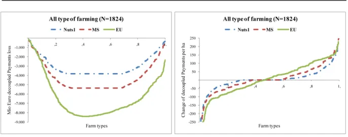
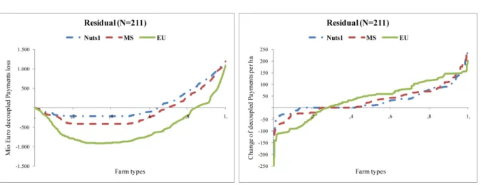
11. The scenario analyses show strong heterogeneous impacts of the introduction of the flat rate among farm types. Particularly negatively affected categories are large and medium-sized farms and dairies, mixed crops and livestock, general field and mixed cropping, olives, cereals and oilseeds and permanent crops. Small farms tend to be less affected. However, sheep, goats and grazing, the residual farm category and mixed livestock farms realise higher premiums and incomes.

12. The results reveal substantial redistributional effects within each farm type. Although a farm type may lose payments on aggregate, not all individual farms included within this group may suffer. For example, dairy farms lose 23.1% (1.133 billion €) of decoupled payments on aggregate in the EU flat-rate scenario in the EU-25. Disaggregating this figure, 60% of the farms represented in the group realise payment decreases equal to -1.4 billion €, whereas 40% of farms realise a payment increase of 0.27 billion €.

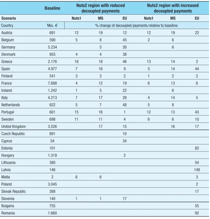
13. By assumption, the Nuts1 and MS flat rate has minor payment redistributional effects between MS. On the contrary, the EU flat-rate scenario has a considerable impact on the redistribution of payments, particularly between the old and new MS. In relative terms, the Netherlands (48%), Belgium (45%) and Greece (44%) experience the highest relative losses, whereas the highest gains are observed in new MS with large land endowments: Latvia (149 %), Romania (92%), Estonia (82%), Bulgaria (55%) and Lithuania (54%). However, Portugal (43%) and Spain (35%) also gain considerable additional payments through a EU-wide flat-rate scheme because of low initial support levels.

(17)

15

Fa

rm l

ev

el po

lic

y s

ce

na

rio a

na

ly

sis

Section 4: WTO Scenario

14. The focus of this scenario is the unique link between a spatial global market model and the farm type supply models. This scenario aims to quantify the impact of a proposal made by the chair of the WTO’s agriculture negotiations, Ambassador Crawford Falconer, in December 2008. He proposed a general tariff reduction based on a tiered formula, a reduction of the TRQ in quota tariffs and the possibility to exclude certain products, called sensitive product

s,

at the cost of the extension of tariff rate quotas for the sensitive-product imports.

15. The simulation results show that tariff reduction increases consumer welfare in the EU by 8.5 billion €, whereas agricultural income decreases by 6.8 billion € (-3%), mainly driven by losses realised in the animal sector that account for 5.5 billion €.

16. Reduced trade protection increases imports and decreases producer and market prices in the EU, in particular for sugar (14%) and beef (13%) but also for butter (10%), cream (5%) and other fruits (5%). 17. The simulation shows that these price reductions translate into relatively small changes in agricultural

production of between 0% and -4% relative to the baseline level. Despite the moderate production change, price reductions directly affect the farm income available to pay for the primary factors such as land and labour.

18. The analysis shows sizable impacts on farm income for different farm types. Generally, farm types specialised in livestock production lose the most. The largest negative income effects were observed for cattle; dairying, rearing and fattening; dairy; mixed crops, livestock; and sheep and goat farm types.

Section 5: Macroeconomic Environment Scenario

19. The macroeconomic environment is an important factor in determining the agricultural sector’s development. We simulate the farm-level effects of a hypothetical economic recovery scenario that may lead to higher GDP growth and higher oil prices. We assume two shocks: an increase in the crude oil price by 50% and an annual world GDP growth rate increase of 1% (or 16% cumulative) compared to baseline.

20. In general, the considered shocks lead to higher commodity prices, and the oil price shock also causes higher production costs. An increase in the annual world GDP growth rate by 1% relative to baseline causes stronger price effects than does the 50% increase in the oil price.

21. With the oil price shock, farmers are affected by two opposing market effects: an increase in production costs and an increase in revenues. In most cases, increasing costs dominate such that the overall farm income declines.

(18)

16

Ex

ec

ut

iv

e S

um

m

ar

y

22. The effect of higher GDP on income across farm types is generally positive due to the increasing demand for agricultural products, which generates an increase in the prices of agricultural commodities. Farmers react to the new macro environment with adjustments of their production. Thus, the effect of the increased GDP leads to an increase in arable land and intensification of crop and animal production activities. Furthermore, a tendency to substitute grassland for arable land can be observed, particularly in farms other than those specialised in cattle or sheep and goat production.

(19)

17

Fa

rm l

ev

el po

lic

y s

ce

na

rio a

na

ly

sis

I. Introduction

Project objective

Consistent with the invitation to tender IPTS-2009-J05-54-RC-AMI, three policy scenarios are evaluated in this report. First, the direct payment scenario is simulated. This scenario investigates the impact of changing from the historical/ hybrid SPS model to a regional SPS model. In the second macroeconomic environment scenario, the recovery from the economic crises and its impact on the agricultural sector are analysed. The third scenario investigates the impact of a WTO proposal. In addition to scenario analysis, the modelling of the CAPRI farm type layer is improved, and the base year data is updated using the most recent available FSS and FADN data. The baseline has been updated for the year 2020, and it is used as a counterfactual situation for the scenario analysis. The report begins with the background description of the CAPRI farm type development conducted within this project, followed by an overview of its characteristics and limitations. Chapter 2 introduces the CAPRI baseline. In Chapter 3, the three scenarios are described, results presented and conclusions drawn.

Background

The CAPRI modelling system was originally developed to analyse policies at the regional level in Europe. Mathematical programming (MP) models were chosen to model policy-induced production changes. Since then, these supply models have been extended continually, now covering the EU-27, Norway, the Western Balkans and Turkey with 273 mathematical programming (MP) models. They are defined at the level of administrative units (Nuts2). The mathematical programming models are conceptually an effective device for explicitly modelling policy

interventions at the farm level, but policies at the market level, such as tariffs, are modelled with the spatial, global, multi-commodity model for agricultural products. This market model covers 60 countries in 28 trade blocks worldwide. Three trading regions cover the EU, namely the EU-15, EU-10 as well as Bulgaria and Rumania (BuR).

The market model is a partial equilibrium model, whereas the supply for the three European regions is simulated by the 273 supply programming models. To link the supply and the market models, the behavioural parameters for supply and feed demand for the countries covered by the supply model are sequentially updated based on the results of the market model. This design makes it possible to explicitly define policies in the mathematical programming models for the EU while allowing for endogenous for agricultural products. One should note that the market model also simulates the demand in the EU and supply, feed and processing demand and human consumption based on specific functional forms for all non-EU regions modelled. An iterative approach is used to balance supply and demand. It starts by using a given price, simulating an EU-wide supply and introducing the supply changes in the form of shocks in the supply part of the market model to obtain a new price. The price is used as an input for the mathematical supply models, and this process is repeated until supply and demand are balanced.

The shift from market to direct payment support starting with the 1992 reform and the introduction of farm-specific premium schemes (e.g., stocking densities and decoupled payments) motivated the development of a tool that is disaggregated at the farm level and is thus able to capture these changes in policies. A farm type module was introduced in the CAPRI model using the FADN (Farm Accountancy Data

(20)

18

I. I

nt

ro

du

ct

io

n

Network) and the FSS (Farm Structure Survey). The FADN is the database most frequently used to source EU farm type models. It comprises single-farm observations of commercial farms on production and sales values, production activity levels, yields for selected activities and input costs as well as information about prices, subsidy payments, farm income and other financial and economic variables. The definitions in FADN are harmonised by EU legislation, which also requires yearly updates of the survey from the EU Member States. The FADN, however, only covers a sample of farms with aggregation weights attached, with a somewhat low representativeness for less frequent farm types and production activities. The second data source, the FSS, mainly reports data on the production activities based on a sub-survey every third year and a complete survey every tenth year. Both data sets exclude small farms based on minimum economic thresholds that vary among Member States, with lower thresholds in the FSS and thus, better representation compared to the FADN. Similarly, some enterprises, such as highly commercialised farms, are not obligated to provide accounting information to the FADN but are included in the FSS. The access to FADN and FSS data and the support of several previous research projects1

made it possible to successfully develop farm group supply models within the CAPRI modelling framework. The farm groups are called “farm types”, and the module is called the CAPRI farm type layer (CAPRI-FT), which consists of 1823 farm supply models. The farm type layer mainly aims to capture heterogeneity in farming specialisation and economic size within a region to reduce aggregation bias in the response of the agricultural sector to policy and market signals. This model extension is especially important when the simulated policy instruments are farm specific, as is the case of the historical SPS, or when the instruments are modulated depending on farm characteristics. Additionally, the farm

1 http://www.capri-model.org/projects.htm

type layer might allow future extension of the model to account for farm structural change.

Characteristics of the farm type layer in

CAPRI

One important characteristic of the CAPRI-FT is its full integration in the CAPRI modelling chain, which ensures that price feedback is based on sequential calibration with the global, large-scale market model (Table 1).

Endogenous prices in the CAPRI-FT are an important advantage relative to other farm models used in the literature. In general, other EU farm models, such as the AROPAj system (Baranger et al., 2008), FARMIS (Offermann et al., 2005) and LUAM (Jones et al., 1995), are representative models for a given EU region. They are simulated based on mathematical modelling and are sourced from the FADN database (similar to CAPRI-FT), but an important weakness is that these models are stand-alone supply models in which prices are assumed to be exogenous. Linking the farm models to existing market models is a challenging task due to data gaps, differences in product definitions, and the mismatch between data sets that are available at the farm level and the underlying market-level data. The strict and consistent top-down consistency of the farm type layer available in CAPRI-FT ensures a harmonised data set across regional scales and farm types.

The farm type supply module in CAPRI consists of independent aggregate nonlinear programming models for each farm type aggregated over all activities belonging to a given farm type and a specific administrative regional unit at the Nuts2 level. In this approach, there is a compromise between a pure LP approach and the fully econometrically estimated one. The compromise is achieved by combining a Leontief technology for variable costs, covering low- and high-yield variants for the different production activities, with a partly econometrically estimated

(21)

19

Fa

rm l

ev

el po

lic

y s

ce

na

rio a

na

ly

sis

behavioural function (Jansson and Heckelei, 2011) based on the positive mathematical programming (PMP) approach (Howitt, 1995). The nonlinear cost function captures the effects of labour and capital on farmers’ decisions. Its advantage is that it allows perfect calibration of the supply models and smooth simulation of responses to policy changes. The farm models, similar to the regional models, capture the premiums paid under the CAP in great detail; they include NPK balances and a module with feeding activities that accounts for the nutrient requirements of animals. In addition to the feed constraint, other model constraints relate to land supply and subsitution between grass and arable land. Prices are exogenous in the supply module, but they are endogenously determined

by the market module in an iterative process solved between the supply and market modules until convergence is reached. Grass, silage and manure are assumed to be non-tradable and are assigned internal prices based on their substitution values and opportunity costs.

The CAPRI farm type module comprises a maximum of nine of the most important farm types per region plus a residual farm type, altogether representing total regional production as well as input and primary factor use. The nine farm groups are characterised along two dimensions (Table 2): (i) by the “type of farming”, determined by the farm production specialisation, as defined by the relative contributions of different production branches to the gross margin

Table 1: Overview of CAPRI - farm type model characteristics

Type of model Independent aggregate non linear programming models

Components of the model Compromise between a pure LP approach and the fully econometrically estimated one, extending PMP

Objective function Maximizing differences between revenues plus premiums minus variable cost and a cost component from the quadratic cost function

Capital and Labour Effects of labour and capital on farmers decisions caught by the cost function Land Endogenous land supply function consists of a three-tier land allocation model that

allocates between agricultural land and land for other uses (e.g., grassland versus arable land) and allocates by land use based on various crop and grassland intensities Nutrient balance NPK balances; feeding activities covering nutrient requirements of animals

Constraints Feed block, total land use, set-aside obligations and quotas Prices

tradable products Are exogenous in the supply module and are provided by the market module, with which they are solved sequentially until convergence.

non-tradable products Grass, silage and manure are assumed to be non-tradable and receive internal prices based on their substitution value and opportunity costs

Calibration of the base year The cost function allows both for perfect calibration of the models and a smooth simulation response

Farm Types in CAPRI

Total No. EU-25 1823

Total no.of supply models 1888

No.per Nuts2 Maximum of nine of the most important farm types per region plus a residual farm group

Integration into CAPRI

Methodology Full integration in the CAPRI modelling chain, which ensures price feedback based on sequential calibration with the global, large-scale market model, strict and consistent top-down disaggregation approach in the baseline; obtaining a harmonised data set across regional scales and farm types

IT Where possible, CAPRI-FT uses the same GAMS routines as the regional supply models

(22)

20

I. I

nt

ro

du

ct

io

n

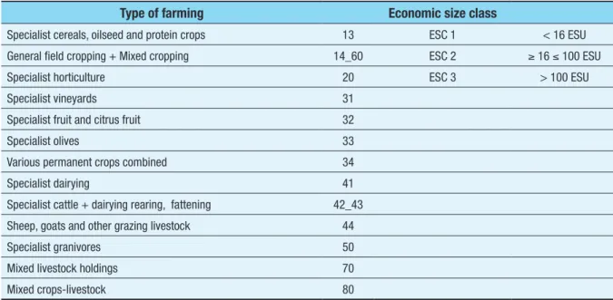
of the farm (European Commission, CD 85/377/ EEC, Article 6) and (ii) the “economic size class” of the farm, represented in terms of “European size units” (ESU). The EU classification scheme allows for a far more detailed characterisation of a farm’s specialisation. The choice of 13 farm specialisations is a compromise between model complexity, robustness of the result, reporting limitations and data constraints. In particular, the data confidentiality issues that are highlighted when using more disaggregated types in regional aggregates render it suitable to adhere to the classification shown in Table 2. Additionally, higher farm disaggregation would increase the complexity of the results without adding value in terms of policy-relevant reporting of the model results. Similar arguments support the use of only three economic farm size classes (ESC), defined as ESC 1 for farms smaller than 16 ESU, ESC 2 for farms of at least 16 ESU but less than 100 ESU, and ESC 3 for farms of 100 ESU or larger. In total, this leads to 13*3=39 cells in the overall farm typology.

From these 39 possible farm types, up to 9 of the most important farm types are selected in each Nuts2 region. The farm selection is based on two criteria: livestock units (LU) and utilised agricultural area (UAA). Both criteria were assigned equal priority (equal weights) in

determining the importance of each farm type. Compared to other weighting systems based on the number of farms, economic indicators, area farmed or livestock numbers, this approach provides a compromise between the economic, social and environmental aspects of farming. For further information on the methodology of the construction of the farm type layer, see Gocht (2010a), (2010b) and Gocht and Britz (2011). The farms that are not represented by the 9 most important farm types are included in the residual farm type. The restriction to 10 farm groups (the 9 most important groups plus the residual farm group) per region is based on storage and computing time considerations as well as the need to keep the database and model outputs at a manageable size for quality control and result analysis.

The CAPRI supply module covers 27 EU Member States and nine non-EU countries, each of which are split into several Nuts2 sub-regions. With the introduction of the farm type layer, a Nuts2 region has at most 10 farm types. The CAPRI-FT covers the EU-25, whereas BuR, due to missing FADN statistics, are represented only by the Nuts2 supply models. In summary, there are 1,888 mathematical supply models for the EU-27 in total; 1,823 are farm type models for the EU-25, and 65 are Nuts2 supply models for BuR.

Table 2: Types of farming and economic size classes for the farm types

Type of farming Economic size class

Specialist cereals, oilseed and protein crops 13 ESC 1 < 16 ESU

General field cropping + Mixed cropping 14_60 ESC 2 ≥ 16 ≤ 100 ESU

Specialist horticulture 20 ESC 3 > 100 ESU

Specialist vineyards 31

Specialist fruit and citrus fruit 32

Specialist olives 33

Various permanent crops combined 34

Specialist dairying 41

Specialist cattle + dairying rearing, fattening 42_43

Sheep, goats and other grazing livestock 44

Specialist granivores 50

Mixed livestock holdings 70

(23)

21

Fa

rm l

ev

el po

lic

y s

ce

na

rio a

na

ly

sis

Limitations of the approach

One of the main drawbacks of the CAPRI-FT approach is the use of structurally identical, stylised and relatively simple template models in which differences between farm types and regions are expressed solely by parameters. This approach might not completely capture the full diversity of farming systems in Europe. In particular, the evaluation of policy measures that impact farm management decisions, such as manure handling or feeding practices, demands models that include these factors as decision variables. The relatively simple representation of agricultural technology in CAPRI compared to approaches that are parameterised based on biophysical models narrows the scope of extensions in that direction. The potential of the current template has not yet been fully exploited in CAPRI, although the dichotomy between increased detail for specific activities, regions and farm types and a structurally identical template model remains. Updating and maintaining a regional database with an additional breakdown by farm type requires more resources, as does the application of the enlarged simulation tool.

Scenario application with the farm type

layer in this study

The scenarios make use of the farm type layer with respect to the explicit and detailed implementation of the SPS (single payment scheme) at the farm type level. Farm-related premium, income and cost effects can thus be analysed also with respect to the type of farming and the economic size. The top-down Pillar 1

distribution, considering the ceilings values from the regulatory texts, across the sector, regions and farm types, provides a complete picture of the premium distribution. In addition, the economic model available behind each farm type ensures that policy impacts on land rents and land-use changes can be analysed. This capability is particularly relevant for the flat-rate scenario. In addition, the unique link between the farm supply models and the agricultural trade model is used to analyse the full range of tariff cuts and CAP measures in the macroeconomic and WTO scenarios at the farm level. For example, in the macroeconomic scenario, impacts of higher GDP growth world wide on global and EU agricultural markets are simulated. This effect, in turn, affects income, production, and input use at the farm level. Note that the response behaviour of the CAPRI farm type model also changes as compared to the CAPRI Nuts2 regional model due to a reduced aggregation error. Farm supply models behave more restrictively than the Nuts2 supply models. Typically, each individual farm type model comprises less activities and thus a smaller production possibility set compared to the more aggregated NUTS2 models. For example, a farm type specialised in cereals, oilseed and protein cannot easily change production specialisation (e.g., to a sheep and goat farm type) due to restrictions in land endowment, education, machinery and other farm resources, even in the presence of price and/or policy incentives. However, if modelled at the regional Nuts2 level, the farm would be less restricted in its ability to adjust its production behaviour because the constraints are aggregated over all farms in the region, thus making more resources available for all of the production activities in the region.

(24)

(25)

23

Fa

rm l

ev

el po

lic

y s

ce

na

rio a

na

ly

sis

II. The Baseline

An important component of the scenario analysis is the CAPRI baseline. The baseline is used as a comparison point for the scenarios. Assumptions underlying and information included in the baseline are discussed in this chapter. First, we briefly motivate the methodology and provide an overview of the different policy and macroeconomic assumptions. A detailed description can be found in Britz & Witzke (2009). The CAPRI baseline construction relies on a combination

of three information sources: the AGLINK baseline2_{, an analysis of historical trends}

and expert information. The most relevant information is a preliminary AGLINK baseline prepared for this project at the IPTS in October 2009. It includes recent assumptions on macroeconomic drivers, such as GDP, population, oil price and the evolution of the CAP, in particular the expiry of the milk quota system. Important economic variables from the baseline are summarised in Table 3.

2 BLANCO FONSECA, M., ET AL.: IPTS Agro-Economic Modeling Platform: Bio fuel Modeling (AGLINK, ESIM, CAPRI). JRC - IPTS, Seville, 2009

Table 3: Comparison between base year and baseline

Base year 2005 Baseline 2020

Political variables

Milk Quota EU-25 in million tonnes 133

Sugar Quota EU-27 in 1.000 tonnes 17.000 12.400

Macroeconomic Assumptions (EU-27)

Population growth in % p.a. - 0,04%

Crude oil price in $ per barrel 38 104

Inflation in % p.a. - 1,90%

Other Trends (EU-27)

New energy crops second generation in 1.000 hectares 0 1.500

Prices for important products (EU-27, €/t)

Cereals 104 140

Oilseeds 202 224

Beef 1.714 2.507

Dairy products 1.282 1.393

Struktural change

EU-25 No. of Holdings in Mio 10,2

constant

EU-15 No. of Holding in Mio 6,6

EU-10 No. of Holding in Mio 3,6

Land Use (EU27, 1000 ha)

Used Agricultural Area 191.272 187.419

Pasture 65.309 64.910

(26)

24

II. T

he B

as

el

in

e

Because the regional resolution of the AGLINK baseline is limited to EU aggregates, the baseline draws additionally on national expert information. Furthermore, the baseline includes specific expert information from the PRIMES energy model for the bio-fuel sector and expert projections from the seed manufacturer KWS for the sugar sector. Trends and expert information combined might be inconsistent and might violate basic technical constraints, such as crop area and/or young animal balances. Consequently, all expert information is usually provided in the form of target values. For consistency reasons (such as production quantity equalisation with activity levels and yields), deviations from target values are allowed; however, to avoid large deviations, they are penalised during the model estimation process. Another important input into the baseline constructions is detailed information on policy measures. The policy assumptions complete the definition of the CAPRI baseline and, together with other data, form the basis of

parameter calibration. The baseline represents the starting point (the counterfactual situation) for the subsequent scenario analysis. Table 4 provides an overview of the policy reforms implemented in the baseline for this study.

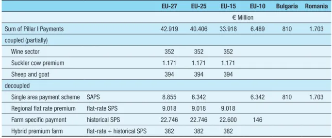
Table 5 summarises the total direct payments on gross value added amongst MS aggregated according to baseline farm types.

Special characteristics of farm types

We now briefly discuss additional assumptions made for the farm type baseline. Generally, it would be desirable to distinguish two different forms of development in the baseline projections for particular farm types: production development (crop allocation and animal herd size) of each farm type and composition, which is the number of farms in a group. This distinction is not possible with the current version, but the

Table 4: Policies included at baseline

Baseline 2020

Common Agriculturel Policy Reforms

.. of the Milk Market milk quota removed

.. of Mid Term Review historical SPS, flat-rate and SAPS for new MS

.. of the Sugar Market Reform of the CMO sugar of 2006 implemented. Sugar quotas fixed on the 2009 values. _{Ethanol beets introduced} .. Helth Check

further decoupling of payments for olive and hops; beef and veal, protein crops, rice; removal set aside obligation; increase of modulation distributed over four steps beginning in 2009;

Table 5: Overview of pillar 1 payments at baseline for different EU aggregates

EU-27 EU-25 EU-15 EU-10 Bulgaria Romania

€ Million

Sum of Pillar I Payments 42.919 40.406 33.918 6.489 810 1.703

coupled (partially)

Wine sector 352 352 352

Suckler cow premium 1.171 1.171 1.171

Sheep and goat 394 394 394

decoupled

Single area payment scheme SAPS 8.855 6.342 6.342 810 1.703

Regional flat rate premium flat-rate SPS 9.018 9.018 9.018

Farm specific payment historical SPS 22.746 22.746 22.600 146 Hybrid premium farm flat-rate + historical SPS 382 382 382

(27)

25

Fa

rm l

ev

el po

lic

y s

ce

na

rio a

na

ly

sis

development of a structural change module that will address these shortcomings is foreseen within the medium-term development of the system. The main constraint for this development is the missing time-series data for the evaluation of farm groups and their production structures to build trend forecasts and expectations for baseline routines. Accordingly, a different approach has been chosen in the current version. The prior information is obtained by multiplying the base period value of a variable of interest (e.g., hectares for a crop, herd sizes, input-output coefficients) for a given farm type by the ratio between the projected value at the Nuts2 level and the Nuts2 base year value of the variable. The following consistency conditions are imposed during the

projection, similar to those used at the Nuts2 level: (1) production and total input use are derived from activity levels and input-output coefficients; (2) the UAA must equal the sum of the crop area; (3) nutrient requirements (protein, energy, different types of fibre) for each animal must be in balance with the deliveries from feeding; (4) own-produced fodder (grass, silage maize, fodder root crops, and other fodder from arable land) must be used within the same farm type; (5) the sum of the crop area and the animals across all farm types must equal Nuts2 values; (6) the sum of the production and input use across all farm types must be equal to Nuts2 values; and (7) the weighted average of feed input coefficients must be equal to those observed at the Nuts2 level. The

Table 6: Indicators for different EU-25 aggregated farm types

EU-25 EU-15 EU-10

No.

of F

arm Supply Models

Utilized Agricultural Area No.

of Holdings

Livestock Units No.

of F

arm Supply Models

of Holdings

Livestock Units No.

of F

arm Supply Models

of Holdings

Livestock Units

Type of Farming No. Million No. Million No. Million

Cereals, oilseed & protein crops 245 32,20 1,00 2,10 173 25,60 0,70 1,90 72 6,60 0,30 0,20

General field & mixed cropping 251 20,00 1,80 3,70 201 14,90 0,90 3,00 50 5,10 0,90 0,70

Dairying 235 16,90 0,50 19,40 205 15,30 0,40 18,50 30 1,70 0,20 0,90

Cattle- Dairying -rearing & fattening 149 11,70 0,40 12,00 133 10,90 0,30 11,60 16 0,80 0,10 0,40

Sheep, goats and other grazing livestock 172 15,50 0,50 6,90 159 15,10 0,40 6,80 13 0,40 0,00 0,10

Granivores 118 2,70 0,20 10,20 76 1,60 0,00 8,80 42 1,00 0,20 1,40

Mixed livestock holdings 85 5,10 0,50 5,10 53 1,80 0,10 3,00 32 3,30 0,40 2,10

Mixed crops-livestock 276 19,80 0,90 13,00 214 12,70 0,30 11,00 62 7,10 0,70 2,00

Vineyards 22 1,40 0,20 0,10 21 1,40 0,20 0,10 1

Fruit and citrus fruit 13 0,60 0,20 0,10 13 0,60 0,20 0,10

Olives 25 3,60 0,80 0,20 25 3,60 0,80 0,20

Permanent crops mixed 16 0,50 0,20 0,10 15 0,50 0,20 0,10 1

Horticulture 5 0,10 5 0,10

Economic Size Class

<=16 ESU 486 36,60 6,00 11,90 342 22,40 3,20 7,50 144 14,20 2,70 4,40

>16 and <=100 ESU 673 56,80 1,00 36,20 602 52,80 1,00 34,70 71 3,90 0,10 1,50

>100 ESU 453 36,60 0,20 24,80 349 28,80 0,20 22,80 104 7,80 2,00

Residual 211 39,50 3,10 16,60 170 32,70 2,30 15,00 41 6,80 0,80 1,50

(28)

26

II. T

he B

as

el

in

e

prior information for the different data elements at the farm type level is defined from the base year results of each farm type and the projected changes over time in the related Nuts2 regions. Generally, all variables are solved simultaneously to account for the interactions between crops

and animals in the estimation procedure. The boundaries surrounding the prior information help to ensure the plausibility of the obtained results. Developments in acreage and herd size based on farm type at baseline are captured by the set of relative changes projected at the Nuts2

Figure 1: Cropping pattern for EU-25 aggregated farm types and EU-25 total

(29)

27

Fa

rm l

ev

el po

lic

y s

ce

na

rio a

na

ly

sis

level. If no feasible solution is found, the limits are relaxed. The approach guarantees identical results for the baseline at the MS and regional Nuts2 levels from model versions both including and excluding particular farm types.

Table 6 shows the number of farm types per type of farming and economic size class

separately for the EU-25, EU-15 and EU-10. In addition, it presents the utilised agricultural area (UAA) and the livestock units (LU) of each farm type at baseline. In addition, the number of holdings each farm type represents is provided. This value is obtained from the base year statistic. Note that the total numbers in the last row of Table 5 are calculated either by adding the residual farm type to all type of farming

rows or by adding the economic size classes. The table shows that specialised cereals, oilseeds and protein crops are represented in the model by 245 supply models, which together represent 32.2 million hectares UAA and 2.1 million LU. In the base year 2005, approximately 1 million farms were represented by this type of farming. Table 6 also indirectly shows the stocking density; in particular, granivores have a very high stocking density of 3.7 LU per hectare of UAA.

In Figure 1 and Figure 2, the compositions of the different farm types with respect to cropping pattern and herd size (in LU) are presented. The pie chart in Figure 1 shows the total land use for the EU-25. Almost half of the land (84.2 million ha) is used for fodder production, which includes maize silage, grassland and other fodder on arable land. Another 42 million ha are cultivated with cereals, 7.9 million ha with fallow land or set aside, 14.5 million ha with vegetables, 8.7 million ha with oilseed and 8.4 million ha with other arable crops, such as potatoes, pulses and sugar beets. In the bar chart, the first twelve bars present the composition of land use per type of farming, while the last four present land use with respect to the economic size class and for the

residual farm type. The land use allocation has a specific composition in each of the farm types. For example, the following farm types mainly

have fodder area under cultivation: dairying; cattle-dairying, rearing and fattening; and sheep, goats and other grazing livestock. However, cereals and other crops are mostly cultivated in specialised cereal farms. Vineyards, fruit, citrus, horticulture and permanent crops mixed farm types are not often represented as specific farm types due to their low importance compared to other farm types at the Nuts2 level in terms of land use and animal stocking density. These farm types are mostly aggregated into the residual farm type, as is shown by the high share of permanent cropping areas in this farm type.

Figure 2 characterises animal production activities measured in livestock units. The total livestock units in the EU-25 are 89.4 million LU (se also Table 6). The animal aggregate of cows, cattle for raising activities and calf fattening, accounts for almost 33 million LU, followed by cattle for beef meat production with 23.8 million LU and veal production, with 22 million LU.

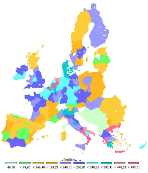
Figure 3 provides an overview of the distribution of the coupled payments per hectare of UAA across the 27 at baseline. In the EU-27, all decoupled payments are more than 50 € per ha (aggregated at the Nuts2 level). Only the Western Balkans (light green area) have a support level that is well below this value.

Several Nuts2 regions in Spain, France, Austria, Latvia and Finland (shown in green) have payments between 50 and 100 €/ha UAA. Regions with a low stocking density and low historical yields (15) receive payments below the EU-27 average of 2EU-27 €/ha. The areas represented in orange, which are regions with payments greater than 100 €/ha but less than 200 €/ha, are below the EU-27 average. Many regions in northern Spain, the South of France, Scotland, Sweden and the majority of regions in the new MS (Poland, Bulgaria, Romania, Estonia and Lithuania) receive similar levels of payments, indicating that a EU-wide flat rate will not only affect regions in the new MS but also some regions in Southern Europe and Scotland. The blue regions receive

(30)

28

II. T

he B

as

el

in

e

payments greater than 200 €/ha and lower than 350 €/ha. The turquoise areas receive payments greater than 350 €/ha and lower than 450 €/ha

UAA. The Netherlands, southern Italy and Greece (olive support) receive the highest payments, at more than 450 €/ha.

(31)

29

Fa

rm l

ev

el po

lic

y s

ce

na

rio a

na

ly

sis

III.

Scenario Analysis

For the current study, three scenarios were analysed: the direct payment scenario, discussed in Section III.1; a macroeconomic scenario, discussed in Section III.2; and the WTO proposal, discussed in Section III.3.

III.1. Direct Payment Scenario

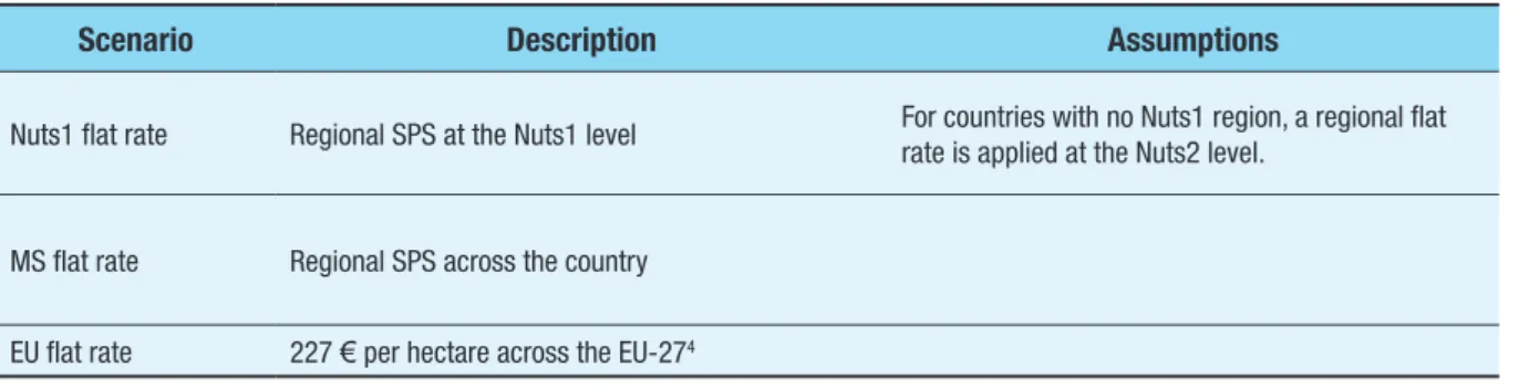
The first scenario is a regional flat rate introduced at the Nuts1 level. In addition, we simulated flat-rate premiums at the MS and EU levels, as summarised in Table 7. The following chapter includes a brief methodological description of how the direct payments are defined and implemented in the model.

Description

The SPS is a payment obtained from the decoupling of direct premiums from production that was introduced as part of the CAP Mid Term Review 20033_{. This payment was distributed to}

farmers in two different ways: 4

3 The EU flat-rate amount (227 €/ha) is calculated by dividing the total EU-27 SPS payments by the UAA at baseline. 4 COUNCIL REGULATION (EC) No 1782/2003 of 29

September 2003 establishes common rules for direct support schemes under the common agricultural policy as well as certain support schemes for farmers and amending regulations.

• First, single payments are calculated at the farm level. Under this scheme, the SPS payments remain farm specific and equal the value of coupled payments received in the reference period. Next, the SPS entitlement value per hectare is calculated by dividing the reference coupled premium endowment by the farm reference area. This SPS model is abbreviated as “historic SPS” in this report. • Second, the total amount of payments is

averaged over a region on a hectare basis. The sum of payments received by all farmers in a particular area during the reference period is divided by the number of eligible hectares in that region. This results in a uniform hectare premium and is abbreviated in this report as “regional SPS”.

The Member States had to opt for one SPS category. The regional SPS could be combined with a farm-specific top-up, which is known as a hybrid SPS scheme. This scheme can be fixed or may vary over time, leading to a so-called

Table 7: Overview of the sub-scenarios for the direct payment scenario

Scenario Description Assumptions

Nuts1 flat rate Regional SPS at the Nuts1 level For countries with no Nuts1 region, a regional flat _{rate is applied at the Nuts2 level.}

MS flat rate Regional SPS across the country EU flat rate 227 € per hectare across the EU-274

(32)

30

III

. S

ce

na

rio A

na

ly

si

s

fixed or dynamic SPS. In the EU-15, ten MS opted solely for the historical SPS, whereas the rest opted for the hybrid flat-rate scheme. In the EU-12, Slovenia and Malta implemented the regional SPS from the beginning, whereas the other nations implemented the Single Area Payment Scheme (SAPS). This is a scheme of a uniform per-hectare payment similar to the regional SPS but without a historical reference area. The SAPS was introduced at 25% from the start of accession (in 2004 for the EU-10 and 2007 for BuR) and gradually increased to 100% over ten years.5

The CAPRI farm type layer allows the shift from a historical SPS to a regional SPS to be analysed. In countries with a historical SPS, farm types have different values for their premium rights depending on the production structure and coupled payments in the reference period. For example, a specialised cattle farm could have received more coupled premiums per hectare due to higher amounts of coupled cattle premiums than another farm type in the region. A shift to a flat-rate scheme in the region would decrease the payments for the cattle farm but increase the payments for other farm types in the region, given that the total amount of SPS in the region is constant. This result would affect the income situation and agricultural markets when land use changes occur. Alongside production and input effects, the flat-rate scheme also alters prices. The price changes are iteratively obtained from the market model in the CAPRI. Thus, the aim of the scenarios is to analyse the redistribution effect and resulting production, price and income changes.

Methodologically, we first calculate all premiums given to a farm type based on information from legal documents, which are mapped onto the production activity units of

5 Note that the new MS are allowed to grant complementary national direct payments (CNDP) to farms up to 30% of the total value of the subsidy ceiling. In the CAPRI model, the CNDP is assumed to be granted until 2013 in the EU-12 and until 2016 in BuR and thus is not included in the 2020 baseline.

the model. The premium amount per production activity is then adjusted considering the available direct payment ceiling in a given region/MS in either monetary terms or in numbers. The SPS implementation in the model is achieved as follows. The level of decoupling determines the total value of SPS in a given region/MS. The total SPS value is then averaged over the Nuts1, MS or EU, depending on the sub-scenario. During the model run, all payments are simulated as endogenous contributions to the objective function, where the sum of payments over all farms is constrained during the iteration to comply with regional premium ceiling values. For each farm type, entitlements are defined as follows: from the reference production in the case of MS-15 and from the baseline production in the case of MS-10, Bulgaria and Romania. If the UAA overshoots the entitlements, the next marginal hectare will not receive the flat-rate premium, and the land market will not be affected by the payment. The entitlements are assumed to be non-tradable between the farm types and regions. Table 8 summarises the SPS implementation at baseline and in the scenarios.

In the EU-15, all historical SPS are moved to a uniform flat rate. In the EU-10, the implementation was not changed for the SAPS, with the exceptions of Slovenia and Malta. Results

We begin with the analysis of the redistribution effects of decoupled payments at different aggregation levels. Next, we present the market impacts of the scenarios on herd sizes, cropping and land use and analyse the effects on agricultural markets and prices. We finish with the farm income analysis.

Redistribution of decoupled payments among EU aggregated farm types

Table 9 presents the redistribution of decoupled payments between different EU

(33)

31

Fa

rm l

ev

el po

lic

y s

ce

na

rio a

na

ly

sis

aggregates. At baseline, the spending on decoupled payments totals 42.8 billion € in the EU-27. The scenario simulations reveal that this level of expenditure does not change much at the EU-27 level in all three flat-rate schemes (-0.7% Nuts1, -0.6% MS and -1% MS flat rate). For the Nuts1 and MS flat-rate scenarios, the respective changes for the 25, 15, EU-10 and BuR are also small. In the EU-15, the changes are driven by market effects (e.g., land use changes and price changes; see below). Most new MS already implement a flat-rate system at baseline (except for Slovenia and

Malta), so there are no redistribution, payment and/or market effects. For the EU flat-rate scenario, approximately 3.15 billion € are redistributed between the EU-15, EU-10 and BuR.6_{The simulations reveal that the EU-15}

will lose -3.4 billion €, whereas the EU-10 and BuR will gain approximately 1 billion € and 1.94 billion €, respectively.

6 This value is obtained as the sum divided by the absolute deviation compared to the baseline and multiplied by 0.5 to obtain the amount of payment flow between regions.

Table 8: Single payment scheme implementation (baseline and scenarios) CAPRI Baseline 2020 Direct payment Scenario CAPRI Baseline

2020 Direct payment Scenario

Countries regional SPS historic SPS Hybrid premium farm flat- rate SPS Countries SAPS regional SPS SAPS regional SPS EU-15 EU-10

Belgium x x Czech Republic x x

Denmark x x x x Estonia x x Germany x x Hungary x x Austria x x Lithuania x x Netherlands x x Latvia x x France x x Poland x x Portugal x x Slovenia x x

Spain x x Slovak Republic x x

Greece x x Cyprus x x Italy x x Malta x x Ireland x x Finland x x x x Sweden x x x x United Kingdom x x x x

Table 9: Redistribution of decoupled payments among EU aggregates EU-Aggregates and MS

Baseline Nuts1 MS EU Nuts1 MS EU

EU-Aggregate Million € change to Baseline % to Baseline

EU-27 42.834 -320 -244 -430,0 -0,7 -0,6 -1,0 EU-25 40.419 -320 -244 -2.371,6 -0,8 -0,6 -5,9 EU-15 33.953 -318 -243 -3.365,5 -0,9 -0,7 -9,9 EU-10 6.466 -1 -1 994,0 -0,0 -0,0 15,4 Bulgaria 755 0 0 415,1 0,0 0,0 55,0 Romania 1.660 0 0 1.526,4 0,0 0,0 91,9

(34)

32

III

. S

ce

na

rio A

na

ly

si

s

In Table 10, the redistribution effects are analysed by farming type for the EU-25.7_Note

that each farm type has a type of farming and an economic size class attribute, except for the residual farm type. Thus, we can analyse the changes by aggregating different types of farming, notwithstanding the economic size class, and vice versa. The total effects can be obtained by considering either all types of farming or all economic size classes together with the residual

farm type.

The level of redistributed payments increases with the increasing regional scope of the implementation (i.e., Nuts1-MS-EU). In relative terms, the biggest gainers are sheep, goats and other grazing livestock, vineyards

and residual farm types. These types receive, on average, low levels of initial support per

7 Bulgaria and Romania have no farm types in the CAPRI-FT; thus, they are not included in tables where results for farm types are presented.

hectare. The biggest losers are olives and

permanent crops mixed because of their high level of initial support. Other farms that lose support are those specialised in cereals, oilseeds and protein crops, general field cropping, dairy farms and mixed crops and livestock as well as large farms. Small farms (less than 16 ESU)are affected little by the flat rate, whereas big farms lose.

Table 11 further disaggregates the results for the EU-15 and EU-10. For the Nuts1 and MS flat-rate scenarios, the value of redistributed payments is almost zero in the EU-10 because of the SAPS, which is also based on a flat-rate payment system. The exceptions are Slovenia and Malta, which implement the historical SPS; thus, small effects are observed in the EU-10. In the EU-15, the redistributional effects are significant because payments vary greatly between farms under the SPS. The redistribution effects for the EU-15 are similar to the figures reported in Table 10.

Table 10: Redistribution of decoupled payments across EU-25 aggregated farm types EU-25

Baseline Nuts1 MS EU Nuts1 MS EU

Type of Farming Million € change to Baseline % to Baseline

Cereals, oilseed & protein crops 7.729 -403 -615 -502,9 -5,2 -8,0 -6,5 General field & mixed cropping 5.423 -415 -580 -963,0 -7,7 -10,7 -17,8

Dairying 4.912 -471 -588 -1.133,1 -9,6 -12,0 -23,1

Cattle- Dairying -rearing & fattening 2.898 124 339 -255,2 4,3 11,7 -8,8 Sheep, goats and other grazing livestock 2.539 560 1.168 971,2 22,1 46,0 38,3

Granivores 640 -37 -37 -41,7 -5,7 -5,7 -6,5

Mixed livestock holdings 1.131 -34 -38 19,4 -3,0 -3,4 1,7

Mixed crops-livestock 5.141 -296 -362 -718,9 -5,8 -7,0 -14,0

Vineyards 196 111 186 112,5 56,6 95,0 57,5

Fruit and citrus fruit 106 9 -20 15,9 8,9 -18,6 15,0

Olives 1.650 -592 -833 -871,7 -35,9 -50,5 -52,8

Permanent crops mixed 203 -51 -58 -86,9 -25,1 -28,8 -42,9

Horticulture 12 4 1 -0,6 29,7 4,3 -5,0

Economic Size Class

<=16 ESU 8.041 -133 101 198,2 -1,7 1,3 2,5

>16 and <=100 ESU 14.471 -803 -582 -1.769,1 -5,6 -4,0 -12,2

>100 ESU 10.068 -555 -956 -1.884,1 -5,5 -9,5 -18,7

(35)

33

Fa

rm l

ev

el po

lic

y s

ce

na

rio a

na

ly

sis

Important regional redistributive effects occur in the EU flat-rate scenario. In the EU-15, almost all farms lose (except for sheep, goats and other grazing livestock, vineyards

and fruit and citrus fruit), whereas in the EU-10 almost all farms gain (except for permanent crops mixed). In Table 9, we report that approximately 1 billion € were channelled to

Table 11: Redistribution of decoupled payments across EU-15/EU-10 aggregated farm types EU-15

Baseline Nuts1 MS EU Nuts1 MS EU

Type of Farming Million € change to Baseline % to Baseline

Cereals, oilseed & protein crops 6.375 -403 -615 -657,8 -6,3 -9,6 -10,3 General field & mixed cropping 4.450 -421 -586 -1.143,0 -9,5 -13,2 -25,7

Dairying 4.590 -446 -564 -1.189,4 -9,7 -12,3 -25,9

Cattle- Dairying -rearing & fattening 2.724 124 340 -261,7 4,6 12,5 -9,6 Sheep, goats and other grazing livestock 2.478 556 1.163 951,0 22,4 47,0 38,4

Granivores 431 -33 -33 -62,1 -7,6 -7,6 -14,4

Mixed livestock holdings 501 -36 -40 -110,9 -7,2 -8,1 -22,1

Mixed crops-livestock 3.728 -300 -366 -919,4 -8,0 -9,8 -24,7

Vineyards 195 111 186 112,4 56,7 95,3 57,6

Fruit and citrus fruit 106 9 -20 15,9 8,9 -18,6 15,0

Olives 1.650 -592 -833 -871,7 -35,9 -50,5 -52,8