Maple: Simplifying SDN Programming
Using Algorithmic Policies
Andreas Voellmy
?Junchang Wang
?†Y. Richard Yang
?Bryan Ford
?Paul Hudak
??Yale University †University of Science and Technology of China
{andreas.voellmy, junchang.wang, yang.r.yang, bryan.ford, paul.hudak}@yale.edu
ABSTRACT
Software-Defined Networking offers the appeal of a simple, cen-tralized programming model for managing complex networks. How-ever, challenges in managing low-level details, such as setting up and maintaining correct and efficient forwarding tables on distributed switches, often compromise this conceptual simplicity. In this pa-per, we present Maple, a system that simplifies SDN programming by (1) allowing a programmer to use a standard programming lan-guage to design an arbitrary,centralizedalgorithm, which we call analgorithmic policy, to decide the behaviors of an entire network, and (2) providing an abstraction that the programmer-defined, cen-tralized policy runs, conceptually, “afresh” on every packet enter-ing a network, and hence is oblivious to the challenge of trans-lating a high-level policy into sets of rules on distributed individ-ual switches. To implement algorithmic policies efficiently, Maple includes not only a highly-efficient multicore scheduler that can scale efficiently to controllers with40+ cores, but more importantly a noveltracing runtime optimizer that can automatically record reusable policy decisions, offload work to switches when possible, and keep switch flow tables up-to-date by dynamically tracing the dependency of policy decisions on packet contents as well as the
environment(system state). Evaluations using real HP switches show that Maple optimizer reduces HTTP connection time by a factor of100at high load. During simulated benchmarking, Maple scheduler, when not running the optimizer, achieves a throughput of over20million new flow requests per second on a single ma-chine, with95-percentile latency under10ms.
Categories and Subject Descriptors: C.2.3 [Computer Com-munication Networks]: Network Operations—Network manage-ment; D.3.4 [Programming Languages]: Processors—Compilers, Incremental compilers, Run-time environments, Optimization.
General Terms:Algorithms, Design, Languages, Performance.
Keywords:Software-defined Networking, Policies, Openflow.
1.
INTRODUCTION
A major recent development in computer networking is the no-tion ofSoftware-Defined Networking(SDN), which allows a net-work to customize its behaviors through centralized policies at a conceptually centralized network controller. In particular, Open-flow [13] has made significant progress by establishing (1) Open-flow tables as a standard data-plane abstraction for distributed switches, (2) a protocol for the centralized controller to install flow rules and query states at switches, and (3) a protocol for a switch to forward to the controller packets not matching any rules in its switch-local flow table. These contributions provide critical components for re-alizing the vision that an operator configures a network by writing
Permission to make digital or hard copies of all or part of this work for personal or classroom use is granted without fee provided that copies are not made or distributed for profit or commercial advantage and that copies bear this notice and the full cita-tion on the first page. Copyrights for components of this work owned by others than ACM must be honored. Abstracting with credit is permitted. To copy otherwise, or re-publish, to post on servers or to redistribute to lists, requires prior specific permission and/or a fee. Request permissions from [email protected].
SIGCOMM’13,August 12–16, 2013, Hong Kong, China. Copyright 2013 ACM 978-1-4503-2056-6/13/08 ...$15.00.
a simple, centralized network control program with a global view of network state, decoupling network control from the complexities of managing distributed state. We refer to the programming of the centralized controller asSDN programming, and a network oper-ator who conducts SDN programming as anSDN programmer, or just programmer.
Despite Openflow’s progress, a major remaining component in realizing SDN’s full benefits is the SDN programming framework: the programming language and programming abstractions. Exist-ing solutions require either explicit or restricted declarative spec-ification of flow patterns, introducing a major source of complex-ity in SDN programming. For example, SDN programming using NOX [8] requires that a programmer explicitly create and manage flow rule patterns and priorities. Frenetic [7] introduces higher-level abstractions but requires restricted declarative queries and poli-cies as a means for introducing switch-local flow rules. However, as new use cases of SDN continue to be proposed and developed, a restrictive programming framework forces the programmer to think within the framework’s - rather than the algorithm’s - structure, leading to errors, redundancy and/or inefficiency.
This paper explores an SDN programming model in which the programmer defines network-wide forwarding behaviors with the application of a high-level algorithm. The programmer simply de-fines a functionf, expressed in a general-purpose programming language, which the centralized controllerconceptuallyruns on ev-ery packet entering the network. In creating the functionf, the programmer does not need to adapt to a new programming model but uses standard languages to design arbitrary algorithms for for-warding input packets. We refer to this model asSDN programming of algorithmic policiesand emphasize that algorithmic policies and declarative policies do not exclude each other. Our system supports both, but this paper focuses on algorithmic policies.
The promise of algorithmic policies is a simple and flexible con-ceptual model, but this simplicity may introduce performance bot-tlenecks if naively implemented. Conceptually, in this model, the functionfis invoked on every packet, leading to a serious compu-tational bottleneck at the controller; that is, the controller may not have sufficient computational capacity to invokefon every packet. Also, even if the controller’s computational capacity can scale, the bandwidth demand that every packet go through the controller may be impractical. These bottlenecks are in addition to the extra la-tency of forwarding all packets to the controller for processing [6]. Rather than giving up the simplicity, flexibility, and expressive power of high-level programming, we introduce Maple, an SDN programming system that addresses these performance challenges. As a result, SDN programmers enjoy simple, intuitive SDN pro-gramming, while achieving high performance and scalability.
Specifically, Maple introduces two novel components to make SDN programming with algorithmic policies scalable. First, it in-troduces a novel SDNoptimizerthat “discovers” reusable forward-ing decisions from a generic runnforward-ing control program. Specifi-cally, the optimizer develops a data structure called a trace tree
that records the invocation of the programmer-suppliedfon a spe-cific packet, and then generalizes the dependencies and outcome to
of a packet, implying that the policy’s output will be the same for any packet with the same value for this field. A trace tree captures the reusability of previous computations and hence substantially reduces the number of invocations offand, in turn, the computa-tional demand, especially whenfis expensive.
The construction of trace trees also transforms arbitrary algo-rithms to a normal form (essentially a cached data structure), which allows the optimizer to achievepolicy distribution: the generation and distribution of switch-local forwarding rules, totally transpar-ently to the SDN programmer. By pushing computation to dis-tributed switches, Maple significantly reduces the load on the con-troller as well as the latency. Its simple, novel translation and dis-tribution technique optimizes individual switch flow table resource usage. Additionally, it considers the overhead in updating flow ta-bles and takes advantage of multiple switch-local tata-bles to optimize network-wide forwarding resource usage.
Maple also introduces a scalable run-time scheduler to com-plement the optimizer. When flow patterns are inherently non-localized, the central controller will need to invokefmany times, leading to scalability challenges. Maple’s scheduler provides sub-stantial horizontal scalability by using multi-cores.
We prove the correctness of our key techniques, describe a com-plete implementation of Maple, and evaluate Maple through bench-marks. For example, using HP switches, Maple optimizer reduces HTTP connection time by a factor of100at high load. Maple’s scheduler can scale with40+ cores, achieving a simulated through-put of over20million requests/sec on a single machine.
The aforementioned techniques have limitations, and hence pro-grammers may write un-scalablef. Worst-case scenarios are that the computation offis (1) not reusable (e.g., depending on packet content), or (2) difficult to parallelize (e.g., using shared states). Maple cannot make every controller scalable, and Maple program-mers may need to adjust their designs or goals for scalability.
The rest of the paper is organized as follows. Section 2 motivates Maple using an example. Section 3 gives an overview of Maple architecture. Sections 4 and 5 present the details of the optimizer and scheduler, respectively. We present evaluations in Section 6, discuss related work in Section 7, and conclude in Section 8.
2.
A MOTIVATING EXAMPLE
To motivate algorithmic policies, consider a network whose pol-icy consists of two parts. First, a secure routing polpol-icy: TCP flows with port 22 use secure paths; otherwise, the default shortest paths are used. Second, a location management policy: the network updates the location (arrival port on ingress switch) of each host. Specifying the secure routing policy requires algorithmic program-ming beyond simple GUI configurations, because the secure paths are computed using a customized routing algorithm.
To specify the preceding policy using algorithmic policies, an SDN programmer defines a functionfto be invoked on every packet
pktarriving atpkt.inport()of switchpkt.switch():
def f(pkt):
srcSw = pkt.switch(); srcInp = pkt.inport() if locTable[pkt.eth_src()] != (srcSw,srcInp): invalidateHost(pkt.eth_src()) locTable[pkt.eth_src()] = (srcSw,srcInp) dstSw = lookupSwitch(pkt.eth_dst()) if pkt.tcp_dst_port() == 22: outcome.path = securePath(srcSw,dstSw) else: outcome.path=shortestPath(srcSw,dstSw) return outcome
The functionfis simple and intuitive. The programmer does not think about or introduce forwarding rules—it is the responsibility of the programming framework to derive those automatically.
Unfortunately, current mainstream SDN programming models force programmers to explicitly manage low-level forwarding rules. Here is a controller using current programming models:
def packet_in(pkt):
srcSw = pkt.switch(); srcInp = pkt.inport() locTable[pkt.eth_src()] = (srcSw,srcInp) dstSw = lookupSwitch(pkt.eth_dst()) if pkt.tcp_dst_port() == 22: (nextHop,path)=securePath(srcSw,dstSw) else: (nextHop,path)=shortestPath(srcSw,dstSw) fixEndPorts(path,srcSw,srcInp,pkt.eth_dst()) for each sw in path:
inport’ = path.inportAt(sw) outport’= path.outportAt(sw) installRule(sw,inport’, exactMatch(pkt), [output(outport’)]) forward(srcSw,srcInp,action,nextHop)
We see that the last part of this program explicitly constructs and installs rules for each switch. The program uses theexactMatch
function to build a match condition that includes all L2, L3, and L4 headers of the packet, and specifies the switch and incoming port that the rule pertains to, as well as the action to forward on portoutport’. Thus, the program must handle the complexity of creating and installing forwarding rules.
Unfortunately, the preceding program may perform poorly, be-cause it uses only exact match rules, which match at a very gran-ular level. Every new flow will fail to match at switch flow tables, leading to a controller RTT. To make matters worse, it may not be possible to completely cover active flows with granular rules, if rule space in switches is limited. As a result, rules may need to be frequently evicted to make room for new rules.
Now, assume that the programmer realizes the issue and decides to conduct an optimization to usewildcardrules. She might replace the exact match rule with the following:
installRule(sw,inport’,
{from:pkt.eth_src(), to:pkt.eth_dst()}, [output(outport’)])
Unfortunately, this program has bugs! First, if a hostAsends a TCP packet that is not to port 22 to another hostB, then rules with wildcard will be installed forAtoBalong the shortest path. If
Alater initiates a new TCP connection to port 22 of hostB, since the packets of the new connection match the rules already installed, they will not be sent to the controller and as a result, will not be sent along the desired path. Second, if initially hostAsends a packet to port 22 ofB, then packets to other ports will be misrouted.
To fix the bugs, the programmer must prioritize rules with appro-priate match conditions. A program fixing these bugs is:
def packet_in(pkt): ...
if pkt.tcp_dst_port() == 22:
(nextHop,path)=securePath(srcSw,dstSw) fixEndPorts(path,srcSw,srcInp,pkt.eth_dst()) for each sw in path:
inport’ = path.inportAt(sw) outport’= path.outportAt(sw) installRule(sw,inport’,priority=HIGH, {from:pkt.eth_src(), to:pkt.eth_dst(),to_tcp_port:22}, [output(output’)]) forward(srcSw,srcInp,action,nextHop) else: (nexthop,path)=shortestPath(srcSw,dstSw) fixEndPorts(path,srcSw,srcInp,pkt.eth_dst()) for each sw in path:
inport’ = path.inportAt(sw) outport’= path.outportAt(sw)
{from:pkt.eth_src(), to:pkt.eth_dst(),to_tcp_port:22}, [output(toController)]) installRule(sw,inport’,priority=LOW, {from:pkt.eth_src(),to:pkt.eth_dst()}, [output(outport’)]) forward(srcSw,srcInp,action,nextHop)
This program is considerably more complex. Consider theelse
statement. Since it handles non port 22 traffic, it installs wildcard rules at switches along the shortest path, not the secure path. Al-though the rules are intended for only non port 22 traffic, since flow table rules do not support negation (i.e., specifying a condition of port != 22), it installs wildcard rules that match all traffic from src to dst. To avoid such a wildcard rule being used by port 22 traffic, it adds a special rule, whose priority (MEDIUM) is higher than that of the wildcard rule, to prevent the wildcard from being applied to port 22 traffic. This is called a barrier rule. Furthermore, the pro-gram may still use resources inefficiently. For example, for some host pairs, the most secure route may be identical to the shortest path. In this case, the program will use more rules than necessary.
Comparing the example programs using the current models with the function f defined at the beginning of this section, we see the unnecessary burden that current models place on programmers, forcing them to consider issues such as match granularity, encod-ing of negation usencod-ing priorities, and rule dependencies. One might assume that the recent development of declarative SDN program-ming, such as using a data query language, may help. But such approaches require that a programmer extract decision conditions (e.g., conditional and loop conditions) from an algorithm and ex-press them declaratively. This may lead to easier composition and construction of flow tables, but it still places the burden on the pro-grammer, leading to errors, restrictions, and/or redundancies.
3.
ARCHITECTURE OVERVIEW
The core objective of Maple is to offer an SDN programmer the abstraction that a general-purpose programf defined by the pro-grammer runs “from scratch” on a centralized controller for ev-ery packet entering the network, hence removing low-level details, such as distributed switch flow tables, from the programmer’s con-ceptual model. A naive implementation of this abstraction, how-ever, would of course yield unusable performance and scalability.
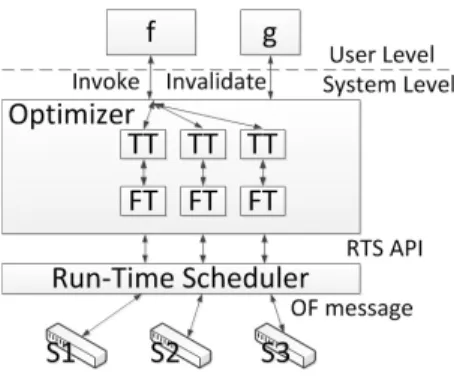
Maple introduces two key components in its design to efficiently implement the abstraction. The first is an optimizer, or tracing run-time, which automatically discovers reusable (cachable) algorith-mic policy executions at runtime, offloads work to switches when possible, and invalidates cached policy executions due to environ-ment changes. One can build a proactive rule installer on top of the tracing runtime, for example, using historical packets, or develop a static analyzer to proactively evaluatef. These are out of the scope of this paper. The second is a run-time scheduler, or scheduler for short, which provides Maple scalable execution of policy “misses” generated by the many switches in a large network on multicore hardware. Figure 1 illustrates the positions of the two components. In addition, Maple allows a set of higher-level tools to be built on top of the basic abstraction: (1) deployment portal, which im-poses constraints on top of Maple, in forms such as best practices, domain-specific analyzers, and/or higher-level, limited configura-tion interfaces to remove some flexibility of Maple; and (2) policy composer, which an SDN programmer can introduce.
This paper focuses on the basic abstraction, the optimizer, and the scheduler. This section sketches a high-level overview of these three pieces, leaving technical details to subsequent sections.
3.1
Algorithmic Policy
fAn SDN programmer specifies the routing of each packet by pro-viding a functionf, conceptually invoked by our run-time
sched-Figure 1: Maple system components.
uler on each packet. An SDN programmer can also provide han-dlers for other events such as switch-related events, but we focus here on packet-arrival events. Although the functionfmay in prin-ciple be expressed in any language, for concreteness we illustratef
in a functional style:
f :: (PacketIn,Env) -> ForwardingPath
Specifically,fis given two inputs:PacketIn, consisting of a packet (Packet) and the ingress switch/port; andEnv, a handle to an environment context. The objective of (Env) is to providef
with access to Maple-maintained data structures, such as a network information base that contains the current network topology.
The return value of a policyfis a forwarding path, which spec-ifies whether the packet should be forwarded at all and if so how. For multicast, this result may be a tree instead of a linear path. The return offspecifies global forwarding behavior through the net-work, rather than hop-by-hop behavior.
Except that it must conform to the signature,fmay use arbitrary algorithms to classify the packets (e.g., conditional and loop state-ments) and compute forwarding actions (e.g., graph algorithms).
3.2
Optimizer
Although a policyfmight in principle follow a different execu-tion path and yield a different result for every packet, in practice many packets—and often many flows—follow the same or simi-lar execution paths in realistic policies. For example, consider the example algorithmic policy in Section 2. fassigns the same path to two packets if they match on source and destination MAC ad-dresses and neither has a TCP port value 22. Hence, if we invokef
on one packet, and then a second packet arrives, and the two pack-ets satisfy the preceding condition, then the first invocation offis reusable for the second packet. The key objective of the optimizer is to leverage these reusable algorithm executions.
3.2.1
Recording reusable executions
The technique used by Maple to detect and utilize reusable exe-cutions of a potentially complex programfis to record the essence of its decision dependencies: the data accesses (e.g., reads and as-sertions) of the program on related inputs. We call a sequence of such data accesses atrace, and Maple obtains traces by logging data accesses made byf.
As an example, assume that the log during one execution of anf
is follows: (1) the only data access of the program is to apply a test on TCP destination port for value 22, (2) the test is true, and (3) the program drops the packet. One can then infer that if the program is again given an arbitrary packet with TCP destination port 22, the program will similarly choose to drop the packet.
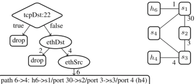
The key data structure maintained by the optimizer is a collection of such data access traces represented as atrace tree. Figure 2 is a trace tree from 3 traces of a programf. In one of these traces, the program first tests TCP destination port for 22 and the result is false (the right branch is false). The program then reads the field value of Ethernet destination (=4) and Ethernet source (=6), resulting in
tcpDst:22 drop true ethDst drop 2 ethSrc
path 6->4: h6->s1/port 30->s2/port 3->s3/port 4 (h4) 6 4 false h6 s1 s2 s4 s3 h4 1 30 3 4
Figure 2: An example trace tree. Diamond indicates a test of some condition, circle indicates reading an attribute, and rectangles contain return values. tcpDst denotes TCP destina-tion; ethDst and ethSrc denote Ethernet destination and source. Topology of the network is shown on the right.
the program’s decision to forward packets from host 6 to host 4 along the shortest path between these two hosts. For concreteness, Figure 2 shows the details of how a path is represented. Assume that host 6 is attached at switch s1/port 1, and host 4 at switch s3/port 4. Figure 2 shows the detail of the path from host 6 to host 4 as: from host 6 (s1/port 1) to output port 30 of s1, which is connected to switch s2; s2 sends out at port 3, which is connected to s3, where host 4 is attached at port 4. The trace tree abstracts away the details offbut still retains its output decisions as well as the decisions’ dependencies on the input packets.
3.2.2
Utilizing distributed flow tables
Merely caching prior policy decisions using trace trees would not make SDN scalable if the controller still had to apply these decisions centrally to every packet. Real scalability requires that the controller be able to “push” many of these packet-level deci-sions out into the flow tables distributed on the individual Openflow switches to make quick, on-the-spot per-packet decisions.
To achieve this goal, the optimizer maintains, logically, a trace tree for each switch, so that the leaves for a switch’s trace tree con-tain the forwarding actions required for that switch only. For exam-ple, for the trace tree shown in Figure 2, the switch-specific trace tree maintained by Maple for switch s1 has the same structure, but includes only port actions for switch s1 at the leaves (e.g., the right most leave is labeled only port 30, instead of the whole path).
Given the trace tree for a switch, the optimizer compiles the trace tree to a prioritized set of flow rules, to form the flow table of the switch. In particular, there are two key challenges to compile an ef-ficient flow table for a switch. First, the table size at a switch can be limited, and hence it is important to produce a compact table to fit more cached policy decisions at the switch. Second, the optimizer will typically operate in an online mode, in which it needs to contin-uously update the flow table as new decisions are cached. Hence, it is important to achieve fast, efficient flow table updates. To address the challenges, our optimizer introduces multiple techniques: (1) it uses incremental compilation, avoiding full-table compilation; (2) it optimizes the number of rules used in a flow table, through both switch-local and network-wide optimizations on switch tables; and (3) it minimizes the number of priorities used in a flow table, given that the update time to a flow table is typically proportional to the number of priority levels [18].
3.2.3
Keeping trace trees, flow tables up-to-date
Just as important as using distributed flow tables efficiently is keeping them up-to-date, so that stale policy decisions are not ap-plied to packets. Specifically, the decision offon a packet depends on not only the fields of the packet, but also other variables. For ex-ample, data accesses byfthrough theEnvhandle to access the net-work information base will also generate dependency, which Maple tracks. Hence, trace trees record the dependencies of prior policy
decisions on not only packet fields but also Maple-maintained en-vironment state such as network topology and configurations.
A change to the environment state may invalidate some part of the trace trees, which in turn may invalidate some entries of the flow tables. There is a large design spectrum on designing the in-validation scheme, due to various trade-offs involving simplicity, performance, and consistency. For example, it can be simple and “safe” to invalidate more flow table entries than necessary—though doing so may impact performance. To allow extensible invalidation design, Maple provides a simple invalidation/update API, in which a flexible selection clause can be specified to indicate the cached computations that will be invalidated. Both system event handlers and user-defined functions (i.e.,gin Figure 1) can issue these API calls. Hence, user-definedfcan introduce its own (persistent) envi-ronment state, and manage its consistency. Note that dependencies that Maple cannot automatically track will require user-initiated in-validations (see Section 4.2) to achieve correctness.
3.3
Multicore Scheduler
Even with efficient distributed flow table management, some frac-tion of the packets will “miss” the cached policy decisions at switches and hence require interaction with the central controller. This controller-side processing of misses must scale gracefully if the SDN as a whole is to scale.
Maple therefore uses various techniques to optimize the con-troller’s scalability, especially for current and future multicore hard-ware. A key design principle instrumental in achieving controller scalability isswitch-level parallelism: designing the controller’s thread model, memory management, and event processing loops to localize controller state relevant to a particular “client” switch. This effectively reduces the amount and frequency of accesses to state shared across the processing paths for multiple client switches.
While many of our design techniques represent “common sense” and are well-known in the broader context of parallel/multicore software design, all of the SDN controllers that we had access to showed major scalability shortcomings, as we explore later in Sec-tion 6. We were able to address most of these shortcomings through a judicious application of switch-level parallelism principles, such as buffering and batching input and output message streams, and appropriate scheduling and load balancing across cores. Section 5 discusses scheduling considerations further.
4.
MAPLE OPTIMIZER
This section details the optimizer, highlighting the construction and invalidation of trace trees and methods for converting trace trees to flow tables. We choose to present out ideas in steps, from basic ideas to optimizations, to make understanding easier.
4.1
Basic Concepts
Trace tree: A trace tree provides an abstract, partial representation of an algorithmic policy. We consider packet attributesa1, . . . an
and writep.afor the value of theaattribute of packetp. We write
dom(a)for the set of possible values for attributea:p.a∈dom(a)
for any packetpand attributea.
DEFINITION1 (TRACETREE). Atrace tree (TT)is a rooted tree where each nodethas a fieldtypetwhose value is one ofL (leaf),V(value),T(test), orΩ(empty) and such that:
1. Iftypet =L, thenthas avaluetfield, which ranges over possible return values of the algorithmic policy. This node represents the behavior of a program that returns valuet without inspecting the packet further.
2. Iftypet=V, thenthas anattrtfield, and asubtreetfield, wheresubtreetis an associative array such thatsubtreet[v]
Algorithm 1:SEARCHTT(t, p)
1 whiletruedo
2 iftypet=Ωthen 3 returnNIL; 4 else iftypet=Lthen
5 returnvaluet;
6 else iftypet=V∧p.attrt∈keys(subtreet)then
7 t←subtreet[p.attrt];
8 else iftypet=V∧p.attrt∈/keys(subtreet)then
9 returnNIL;
10 else iftypet=T∧p.attrt=valuetthen 11 t←t+;
12 else iftypet=T∧p.attrt6=valuetthen 13 t←t−;
is a trace tree for valuev∈keys(subtreet). This node rep-resents the behavior of a program that if the supplied packet
psatisfiesp.attrt=v, then it continues tosubtreet[v]. 3. Iftypet =T, thenthas anattrtfield, avaluetfield, such
thatvaluet ∈ dom(attrt), and two subtree fieldst+ and
t−. This node reflects the behavior of a program that tests the assertionp.attrt = valuetof a supplied packetpand then branches tot+if true, andt−otherwise.
4. Iftypet = Ω, thenthas no fields. This node represents arbitrary behavior (i.e., an unknown result).
Given a TT, one can look up the return value of a given packet, or discover that the TT does not include a return value for the packet. Algorithm 1 shows theSEARCHTT algorithm, which defines the semantics of a TT. Given a packet and a TT, the algorithm traverses the tree, according to the content of the given packet, terminating at anLnode with a return value or anΩnode which returnsNIL.
Flow table (FT): A pleasant result is that given a trace tree, one can generate an Openflow flow table (FT) efficiently.
To demonstrate this, we first model an FT as a collection ofFT rules, where each FT rule is a triple(priority, match, action), wherepriorityis a natural number denoting its priority, with the larger the value, the higher the priority;matchis a collection of zero or more (packet attribute, value) pairs, andactiondenotes the forwarding action, such as a list of output ports, orToController, which denotes sending to the controller. Matching a packet in an FT is to find the highest priority rule whosematchfield matches the packet. If no rule is found, the result isToController. Note that FT matches do not support negations; instead, priority ordering may be used to encode negations (see below).
Trace tree to forwarding table: Now, we describeBUILDFT(t), a simple algorithm shown in Algorithm 2 that compiles a TT rooted at nodetinto an FT by recursively traversing the TT. It is simple because its algorithm structure is quite similar to the standard in-order tree traversal algorithm. In other words, the elegance of the TT representation is that one can generate an FT from a TT using basically simple in-order tree traversal.
Specifically, BUILDFT(t), which starts at line 1, first initial-izes the globalpriority variable to 0, and then starts the recur-siveBUILDprocedure. Note that each invocation ofBUILDis pro-vided with not only the current TT nodet, but also a match param-eter denotedm, whose function is to accumulate attributes read or positively tested along the path from the root to the current node
t. We can see thatBUILDFT(t)startsBUILD withmbeingany
(i.e., match-all-packets). Another important variable maintained by
BUILDispriority. One can observe an invariant (lines 8 and 16)
Algorithm 2:BUILDFT(t) 1 AlgorithmBUILDFT(t) 2 priority←0; 3 BUILD(t,any); 4 return; 5 ProcedureBUILD(t,m) 6 iftypet=Lthen
7 emitRule(priority, m,valuet); 8 priority←priority+ 1;
9 else iftypet=V then
10 forv∈keys(subtreest)do
11 BUILD(subtreest[v], m∧(attrt:v)); 12 else iftypet=T then
13 BUILD(t−, m);
14 mt=m∧(attrt:valuet);
15 emitRule(priority, mt,ToController);
16 priority←priority+ 1;
17 BUILD(t+, mt);
that its value is increased by one after each output of an FT rule. In other words,BUILDassigns each FT rule with a priority identical to the order in which the rule is added to the FT.
BUILDprocesses a nodetaccording to its type. First, at a leaf node, BUILD emits an FT rule (at line 7) with the accumulated matchmand the designated action at the leaf node. The priority of the FT rule is the current value of the global variablepriority. Second, at aVnode (line 9),BUILDrecursively emits the FT rules for each subtree branch. Before proceeding to branch with valuev,
BUILDadds the condition on the branch (denotedattrt:value) to
the current accumulated matchm. We writem1∧m2to denote the intersection of two matches.
The third case is aTnodet. One might think that this is similar to aV node, except that aTnode has only two branches. Un-fortunately, flow tables do not support negation, and henceBUILD
cannot include the negation condition in the accumulated match condition when recursing to the negative branch. To address the issue,BUILDuses the following techniques. (1) It emits an FT rule, which we call thebarrierrule for thetnode, with action being
ToControllerand matchmtbeing the intersection of the assertion
of theTnode (denoted asattrt : valuet) and the accumulated
matchm. (2) It ensures that the barrier rule has a higher priority than any rules emitted from the negative branch. In other words, the barrier rule prevents rules in the negated branch from being ex-ecuted whenmt holds. (3) To avoid that the barrier rule blocks
rules generated from the positive branch, the barrier rule should have lower priority than those from the positive branch. Formally, denoterbas the barrier rule at aTnode,r−a rule from the
nega-tive branch, andr+a rule from the positive branch. BUILDneeds to enforce the following ordering constraints:
r−→rb→r+, (1)
wherer1→r2means thatr1has lower priority thanr2.
SinceBUILDincreases priority after each rule, enforcing the pre-ceding constraints is easy: in-order traversal, first negative and then positive. One can verify that the run-time complexity ofBUILDFT(t) isO(n), wherenis the size of the trace tree rooted att.
Example: We applyBUILDFT to the root of the trace tree shown in Figure 2, for switch s1 (e.g., leaves containing only actions per-taining to s1, such as drop and port 30). Since the root of the tree is aTnode, testing on TCP destination port 22,BUILD, invoked byBUILDFT, goes to line 12. Line 13 recursively callsBUILDon the negative (right) branch with matchmstill beingany. Since the node (labeled ethDst) is aVnode on the Ethernet destination
attribute,BUILDproceeds to visit each subtree, adding a condition to match on the Ethernet destination labeled on the edge to the sub-tree. Since the subtree on edge labeled 2 is a leaf,BUILD(executing at line 7) emits an FT rule with priority 0, with a match on Ether-net destination 2. The action is to drop the packet. BUILDthen increments the priority, returns to the parent, and visits the subtree labeled 4, which generates an FT rule at priority level 1 and in-crements the priority. After returning from the subtree labeled 4,
BUILDbacktracks to theTnode (tcpDst:22) and outputs a barrier rule with priority 2, with match being the assertion of the node: matching on TCP destination port 22. BUILDoutputs the final FT rule for the positive subtree at priority 3, dropping packets to TCP destination port 22. The final FT for switch s1 is:
[ (3, tcp_dst_port=22 , drop),
(2, tcp_dst_port=22 , toController), (1, eth_dst=4 && eth_src=6, port 30),
(0, eth_dst=2 , drop)]
If one examines the FT carefully, one may observe some ineffi-ciencies in it, which we will address in Section 4.3. A key at this point is that the generated FT is correct:
THEOREM1 (FTCORRECTNESS). treeandBUILDFT(tree) encode the same function on packets.
4.2
Trace Tree Augmentation & Invalidation
With the preceding basic concepts, we now describe our tracing runtime system, to answer the following questions: (1) how does Maple transparently generate a trace tree from an arbitrary algo-rithmic policy? (2) how to invalidate outdated portions of a trace tree when network conditions change?
Maple packet access API: Maple builds trace trees with a sim-ple requirement from algorithmic policies: they access the values of packet attributes and perform boolean assertions on packet at-tributes using the Maple packet access API:
readPacketField :: Field -> Value testEqual :: (Field,Value) -> Bool ipSrcInPrefix :: IPPrefix -> Bool ipDstInPrefix :: IPPrefix -> Bool
The APIs simplify programming and allow the tracing runtime to observe the sequence of data accesses and assertions made by a pol-icy. A language specific version of Maple can introduce wrappers for these APIs. For example,pkt.eth_src()used in Section 2 is a wrapper invokingreadPacketFieldon Ethernet source.
Trace: Each invocation of an algorithmic policy that uses the packet access API on a particular packet generates atrace, which consists of a sequence oftrace items, where each trace item is either aTest
item, which records an assertion being made and its outcome, or a
Readitem, which records the field being read and the read value. For example, if a program callstestEqual(tcpDst, 22)on a packet and the return is false, aTestitem with assertion of TCP destination port being 22 and outcome being false is added to the trace. If the program next callsreadPacketField(ethDst)
and the value 2 is returned, aRead item with field being Ethernet destination and value being 2 will be appended to the trace. As-sume that the program terminates with a returned action of drop, then drop will be set as the returned action of the trace, and the trace is ready to be added to the trace tree.
Augment trace tree with a trace: Each algorithmic policy starts with an empty trace tree, represented asΩ. After collecting a new trace, the optimizeraugmentsthe trace tree with the new trace. The AUGMENTTT(t,trace)algorithm, presented in Algorithm 3, adds a new tracetraceto a trace tree rooted at nodet. The algorithm walks the trace tree and the trace in lock step to find the location at which to extend the trace tree. It then extends the trace tree
at the found location with the remaining part of the trace. The algorithm useshead(trace)to read the first item of a trace, and
next(trace)to remove the head and return the rest. The algorithm uses a straightforward procedure TRACETOTREE(trace), which we omit here, that turns a linear list into a trace tree.
Algorithm 3:AUGMENTTT(t, trace)
1 iftypet= Ωthen
2 t←TRACETOTREE(trace);
3 return;
4 repeat
5 item=head(trace);trace←next(trace); 6 iftypet=Tthen
7 ifitem.outcomeis truethen
8 iftypet+= Ωthen
9 t+←TRACETOTREE(trace);
10 return;
11 else
12 t←t+;
13 else
14 iftypet−= Ωthen
15 t−←TRACETOTREE(trace);
16 return;
17 else
18 t←t−;
19 else iftypet=Vthen
20 ifitem.value∈keys(subtreet)then 21 t←subtreet[item.value]; 22 else
23 subtreet[item.value]←TRACETOTREE(trace);
24 return;
25 until;
Example: Figure 3 illustrates the process of augmenting an ini-tially empty tree. The second tree results from augmenting the first tree with traceTest(tcpDst,22; False),Read(ethDst; 2); ac-tion=drop. In this step, AUGMENTTT calls TRACETOTREEat the root. Note that TRACETOTREEalways places anΩnode in an un-explored branch of aTnode, such as thet+branch of the root of the second tree. The third tree is derived from augmenting the sec-ond tree with the traceTest(tcpDst,22; False),Read(ethDst; 4),
Read(ethSrc,6); action=port 30. In this case, the extension is at aVnode. Finally, the fourth tree is derived by augmenting the third tree with traceTest(tcpDst,22; True); action=drop. This step fills in the positive branch of the root.
Correctness: The trace tree constructed by the preceding algorithm returns the same result as the original algorithmic policy, when there is a match. Formally, we have:
THEOREM2 (TT CORRECTNESS). Lettbe the result of aug-menting the empty tree with the traces formed by applying the algo-rithmic policyfto packetspkt1. . . pktn. Thentsafely represents fin the sense that ifSEARCHTT(t, pkt)is successful, then it has the same answer asf(pkt).
Optimization: trace compression: A trace may have redundancy. Specifically, although the number of distinct observations that a programfcan make of the packet is finite, a program may repeat-edly observe or test the same attribute (field) of the packet, for ex-ample during a loop. This can result in a large trace, increasing the cost of tracing. Furthermore, redundant trace nodes may increase the size of the trace tree and the number of rules generated.
Maple appliesCOMPRESSTRACE, Algorithm 4, to eliminate both read and test redundancy in a trace before applying the preceding augmentation algorithm. In particular, the algorithm tracks the sub-set of packets that may follow the current trace. When it encounters
Ω (a) tcpDst:22 Ω true ethDst drop 2 false (b) tcpDst:22 Ω true ethDst drop 2 ethSrc port 30 6 4 false (c) tcpDst:22 drop true ethDst drop 2 ethSrc port 30 6 4 false (d)
Figure 3: Augmenting a trace tree for switch s1. Trace tree starts as empty (Ω) as (a). Algorithm 4:COMPRESSTRACE()
1 fornext access entry on attributeado
2 ifrange(entry) included in knownRangethen
3 ignore
4 else
5 updateknownRange
a subsequent data access, it determines whether the outcome of this data access is completely determined by the current subset. If so, then the data access is ignored, since the program is equivalent to a similar program that simply omits this redundant check. Otherwise, the data access is recorded and the current subset is updated.
Maple trace tree invalidation API: In addition to the preceding packet access API, Maple also provides an API to invalidate part of a trace tree, whereSelectionClausespecifies the criteria:
invalidateIf :: SelectionClause -> Bool
For example, theinvalidateHostcall in the motivating ex-ample shown in Section 2 is a shorthand of invokinginvalidateIf
withSelectionClauseas source or destination MAC addresses equal to a host’s address. This simple call removes all outdated for-warding actions involving the host after it changes location.
As another example, ifSelectionClausespecifies a switch and port pair, then all paths using the switch/port pair (i.e., link) will be invalidated. This topology invalidation is typically invoked by a Maple event listener that receives Openflow control events. Maple also contains an API to update the trace tree to implement fast-routing. This is out of scope of this paper.
4.3
Rule & Priority Optimization
Motivation: With the basic algorithms covered, we now present optimizations. We start by revisiting the example that illustrates
BUILDFT at the end of Section 4.1. LetFTBdenote the example FT
generated. Consider the following FT, which we refer asFTO:
[ (1, tcp_dst_port=22 , drop), (0, eth_dst==4 && eth_src==6, port 30),
(0, eth_dst==2 , drop)]
One can verify that the two FTs produce the same result. In other words, the example shows thatBUILDFT has two problems: (1) it may generate more flow table rules than necessary, since the barrier rule inFTBis unnecessary; and (2) it may use more priority levels
than necessary, sinceFTBhas 4 priorities, whileFTOhas only 2.
Reducing the number of rules generated for an FT is desirable, because rules are often implemented in TCAMs where rule space is limited. Reducing the number of priority levels is also benefi-cial, because TCAM update algorithms often have time complexity linear in the number of priority levels needed in a flow table [18].
Barrier elimination: We start with eliminating unnecessary bar-rier rules.BUILDFT outputs a barrier rule for eachTnodet. How-ever, if the rules emitted from the positive brancht+ oftis
com-plete(i.e., every packet matchingt+’s match condition is handled byt+’s rules), then there is no need to generate a barrier rule for
t, as the rules fort+already match all packets that the barrier rule
would match. One can verify that checking this condition elimi-nates the extra barrier rule inFTB.
Define a general predicateisComplete(t)for an arbitrary tree nodet: for anLnode,isComplete(t) = true, since aBUILDFT derived compiler will generate a rule for the leaf to handle exactly the packets with the match condition; for aVnode,isComplete(t) =
trueif both|subtreest|=|dom(attrt)|andisComplete(subtreev)
for eachv∈keys(subtreest); otherwiseisComplete(t) =false
for theVnode. For aTnodet,isComplete(t) =isComplete(t−). We defineneedsBarrier(t)at aTnodetto be true ift+ is not complete andt−is notΩ, false otherwise.
Priority minimization: Minimizing the number of priorities is more involved. But as we will show, there is a simple, efficient algorithm achieving the goal, without the need to increase priority after outputting every single rule, asBUILDFT does.
Consider the following insight: since rules generated from dif-ferent branches of aVnode are disjoint, there is no need to use priority levels to distinguish them. Hence, the priority increment from 0 to 1 byBUILDFT for the example at the end of Section 4.1 is unnecessary. The preceding insight is a special case of the gen-eral insight: one can assign arbitrary ordering to two rules if their match conditions are disjoint.
Combining the preceding general insight with the ordering con-straints shown in Equation (1) in Section 4.1, we define the minimal priority assignment problem as choosing a priority assignmentPto rules with the minimal number of distinct priority values:
minimize
P |P|
subject to (ri→rj)∧(ri, rjoverlap) :P(ri)< P(rj)
(2)
One may solve Problem (2) using topological ordering. Specif-ically, construct a directed acyclic graph (DAG)Gr = (Vr, Er),
whereVris the set of rules, andErthe set of ordering constraints
among the rules: there is an edge fromritorj iffri → rjand ri, rjoverlap. Initialize variablepriorityto 0. Assign rule
priori-ties as follows: select all nodes without any incoming edges, assign thempriority, delete all such nodes, increasepriorityby 1, and then repeat until the graph is empty.
An issue of the preceding algorithm is that it needs to first gen-erate all rules, compute their ordering constraints, and then assign priorities. However, Maple’s trace tree has special structures that allow us to make simple changes toBUILDFT to still use in-order trace tree traversal to assign minimal priority levels. The algorithm that we will design is simple, more efficient, and also better suited for incremental updates.
Define a weighted graphGo(Vo, Eo, Wo)for a trace tree to
cap-ture all ordering constraints. Specifically,Vois the set of all trace
tree nodes. All edges of the trace tree, except those from aTnode
t tot−, belong toEo as well. To motivate additional edges in Eo, consider all ordering constraints among the rules. Note that
the edges of a trace tree do not include constraints of the form
r−→rb, as defined in Equation (1). To introduce such constraints
inGo, extendEoto includeup-edgesfrom rule-generating nodes
(i.e.,Tnodes with barriers orLnodes). Identifying the up-edges from a rule-generating nodenis straightforward. Consider the path
from the tree root to noden. Consider eachTnodetalong path. If
nis on the negative branch oftand the intersection of the accumu-lated match conditions oft+andnis nonempty, then there should be an up-edge fromntot. One can verify thatGois a DAG.
To remove the effects of edges that do not convey ordering con-straints, we assign all edges weight 0 except the following:
1. For an edge from aTnodettot+, this edge hasw(e) = 1 iftneeds a barrier andw(e) = 0otherwise;
2. For each up-edge, the weight is 1.
Example: Figure 4 showsGo for Figure 3(d). Dashed lines are
up-edges ofEo. Edges that are in both the TT andEoare shown as
thick solid lines, while edges that are only in TT are shown as thin solid lines.Eoedges with weight 1 are labeledw= 1. Thedrop
leaf in the middle has an up-edge to the root, for example, because its accumulated match condition isethDst: 2, which overlaps the root’s positive subtree match condition oftcpDst : 22. TheEo
edge to the positive subtree of the root has weight 0, because the root node is complete and hence no barrier is needed for it.
tcpDst:22 drop true ethDst drop 2 ethSrc port 30 6 4 false w= 1 w= 1
Figure 4: Order graphGofor trace tree of Figure 3(d). Algorithm: The algorithm based onGo to eliminate barriers and
minimize priorities is shown inOPTBUILDFT. The algorithm tra-verses the TT in-order, the same asBUILDFT. Each TT nodethas a variablepriority(t), which is initialized to0, and is incremented as the algorithm runs, in order to be at least equal to the priority of a processed nodexplus the link weight fromxtot. Since all non-zero weight edges flow from right to left (i.e., negative to positive) inGo, in-order traversal guarantees that when it is time to output a
rule at a node, all nodes before it in the ordering graph have already been processed, and hence the node’s priority is final.
Example 1: Consider executingOPTBUILDFT on the example of Figure 4. The algorithm begins by processing the negative branch of the root. At theethDstVnode,OPTBUILDFT updates the pri-ority of its two children with pripri-ority 0, since its pripri-ority is 0 and the edge weights to its children are 0. The algorithm then processes thedropleaf forethDst: 2, emits a rule at priority 0, and updates the root priority to 1, since its priority is 0 and its up-edge weight is 1. The algorithm then processes theethDst : 4branch where it processes the leaf in a similar way. After backtracking to the root,OPTBUILDFT skips the barrier rule, since its positive subtree is complete, and updates the priority of its positive child to be 1 (its priority), since the edge weight to the positive child is 0. Finally, it proceeds to the positive child and outputs a drop rule at priority 1.
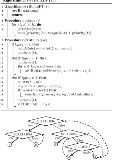
Example 2: Consider the following policy that tests membership of the IP destination of a packet in a set of IP prefixes:
f(p): if p.ipDstInPrefix(103.23.0.0/16): if p.ipDstInPrefix(103.23.3.0/24): return a else: return b if p.ipDstInPrefix(101.1.0.0/16): return c if p.ipDstInPrefix(101.0.0.0/13): return d return e
Algorithm 5:OPTBUILDFT(t)
1 AlgorithmOPTBUILDFT(t)
2 OPTBUILD(t,any);
3 return;
4 Procedureupdate(t)
5 for (t, x)∈Eodo
6 priority(x) =
max(priority(x),weight(t, x) +priority(t));
7 ProcedureOPTBUILD(t,m)
8 iftypet=Lthen
9 emitRule(priority(t), m,valuet); 10 update(t);
11 else iftypet=V then
12 update(t);
13 forv∈keys(subtreest)do
14 OPTBUILD(subtreest[v], m∧(attrt:v));
15 else iftypet=Tthen 16 BUILD(t−, m);
17 mt=m∧(attrt:valuet);
18 ifneedsBarrier(t)then
19 emitRule(priority(t), mt,ToController);
20 update(t); 21 OPTBUILD(t+, mt); 103.23.0.0/16 103.23.3.0/24 a true b false true 101.1.0.0/16 c true 101.0.0.0/13 d true e false false false
Figure 5: Trace tree from an IP prefix matching example.
An example trace tree of this program is shown in Figure 5, which also shows theGo edges for this TT. By avoiding barrier
rules and by using the dependency graph to limit priority incre-ments, OPTBUILDFT generates the following, optimal prioritiza-tion: 2, ipDst:103.23.3.0/24 --> a 2, ipDst:101.1.0.0/16 --> c 1, ipDst:101.23.0.0/16 --> b 1, ipDst:101.0.0.0/13 --> d 0, * --> e
4.4
Efficient Insertion and Invalidation
We now adapt the algorithms of the preceding sections to be-come incremental algorithms, which typically update rules by ex-amining only a small portion of a trace tree, rather than compiling the entire trace tree “from scratch”. Maple allows efficient updates because of information maintained inGo, which we call node
an-notations of the tree.
First consider augmenting a trace tree with a new trace. We mod-ify AUGMENTTT to accumulate the identities ofTnodes when the trace follows the negative branch. After attaching the new trace, we build rules starting with the priority stored at the attachment point. Since building rules for the new trace may increase the priorities of some of theTnodes accumulated above, we modify augmentation to backtrack towards the root and rebuild any positive sub-branches of thoseTnodes along this path whose priorities have increased. Note that the method avoids recompiling branches atVnodes other than the branch being augmented. It also avoids recompiling nega-tive branches of posinega-tiveTancestors of the augmentation point.
Algorithm 6:ROUTEAGGREGATION(ft)
1 Safe elimination of rules inftthat have actionToController;
2 foreach destinationdmentioned inftdo
3 act =action of lowest priority rule inftoverlapping
destinationd;
4 p=priority of highest priority rule that overlaps packets
todand agrees withactand such that all lower priority rules overlapping with packets todagree withact;
5 Delete rules at priority≤pmatching on destinationd
fromft;
6 emitRule(p,matchForDest(d),act);
Invalidation is also simple, because the node annotations pro-vide sufficient information to reconstruct the flow rules generated through a series of updates, even if a full compilation would assign priorities differently. Hence the invalidation of a part of a tree sim-ply involves obtaining the previously-generated rules for that part, leaving all other parts of the tree intact.
4.5
Optimization for Distributed Flow Tables
Maple further optimizes flow table usage through network-wide optimizations, by considering network properties. Below we spec-ify two such optimizations that Maple conducts automatically.
Elimination ofToControllerat network core: To motivate the idea, consider converting the global trace tree in Figure 2 to switch trace trees. Consider the trace tree for a switch s4, which is not on the path from host 6 to 4. If a packet from 6 to 4 does arrive at switch s4, a general, safe action should beToController, to handle the exception (e.g., due to host mobility). Now Maple uses network topology to know that switch s4 is a core switch (i.e., it does not have any connection to end hosts). Then Maple is assured that the exception will never happen, and hence there is no need to generate theToControllerrule for switch s4. This is an example of the general case that core switches do not see “decision misses”, which are seen only by edge switches. Hence, Maple does not install
ToControllerrules on core switches and still achieves correctness. Maple can conduct further analysis on network topologies and the trace trees of neighboring switches to remove unnecessary rules from a switch.
Route aggregation: The preceding step prepares Maple to con-duct more effectively a second optimization which we call route aggregation. Specifically, a common case is that routing is only destination based (e.g., Ethernet, IP or IP prefix). Hence, when the paths from two sources to the same destination merge, the remain-ing steps are the same. Maple identifies safe cases where multiple rules to the same destination can be replaced by a single, broader rule that matches on destination only. Algorithm 6 shows the de-tails of the algorithm. The elimination of rules withToController
as action improves the effectiveness of the optimization, because otherwise, the optimization will often fail to find agreement among overlapping rules.
THEOREM 3. ROUTEAGGREGATIONdoes not alter the forward-ing behavior of the network, provided rules at forward-ingress ports include all generated rules with actionToController.
5.
MAPLE MULTICORE SCHEDULER
Even with the preceding optimizations, the Maple controller must be powerful and scalable enough to service the “cache misses” from a potentially large number of switches. Scalability and parallelism within the controller are thus critical to achieving scalability of the SDN as a whole. This section outlines key details of our imple-mentation, in particular, on the scheduler, to achieve graceful scal-ability. A technical report offers more details [22].
Programming language and runtime: While Maple’s architec-ture is independent of any particular language or runtime infras-tructure, its exact implementation will be language-dependent. Our current system allows a programmer to define an algorithmic policy
fin either Haskell or Java. In this paper, we focus on implement-ingfin Haskell, using the Glasgow Haskell Compiler (GHC). We explore the scheduling offon processor cores, efficiently manag-ing message buffers, parsmanag-ing and serializmanag-ing control messages to reduce memory traffic, synchronization between cores, and syn-chronization in the language runtime system.
Affinity-based, switch-level scheduling offon cores: Consider application offat the controller on a sequence of packets. One can classify these packets according to the switches that originated the requests. Maple’s scheduler uses affinity-based, switch-level paral-lel scheduling. Processing byfof packets from the same switch is handled by a single, lightweight level thread from a set of user-level threads atop of a smaller set of CPU cores [11, 12]. The sched-uler maintains affinity between lightweight threads and hardware cores, shifting threads between cores only in response to persistent load imbalances. This affinity reduces the latency introduced by transferring messages between cores, and enables threads serving “busy” switches to retain cached state relevant to that switch.
This design provides abundant fine-grained parallelism, based on two assumptions. First, a typical network includes many more switches than the controller has cores. Second, each individual switch generates request traffic at a rate that can easily be processed by a single processor core. We expect these assumptions to hold in realistic SDN networks [14].
Achieving I/O scalability: Bottlenecks can arise due to synchro-nization in the handling of I/O operations. To achieve I/O scala-bility, Maple further leverages its thread-per-switch design by en-suring that each OS-level thread invokes I/O system calls (read,
write, andepollin this case) on sockets for switches currently assigned to that particular core. Since the scheduler assigns each switch to one core at a time, this affinity avoids I/O-related con-tention on those sockets both at application level and within the OS kernel code servicing system calls on those sockets.
Further, Maple internally processes messages in batches to han-dle the issue that an OpenFlow switch typically sends on a TCP stream many short, variable-length messages preceded by a length field, potentially requiring two expensive readsystem calls per message. By reading batches of messages at once, and sending batches of corresponding replies, Maple reduces system call costs. Large batchedreadoperations often leave the head of a switch’s message stream in between message boundaries. This implies that using multiple user-level threads to process a switch’s message stream would cause frequent thread stalls while one thread waits for the parsing state of a previous parsing thread to become avail-able. Large non-atomicwriteoperations cause similar problems on the output path. However, since Maple dedicates a thread to each switch, its switch-level parallelism avoids unnecessary syn-chronization and facilitates efficient request batching.
6.
EVALUATIONS
In this section, we demonstrate that (1) Maple generates high quality rules, (2) Maple can achieve high throughputs on augmenta-tion and invalidaaugmenta-tion, and (3) Maple can effectively scale controller computation over large multicore processors.
6.1
Quality of Maple Generated Flow Rules
We first evaluate if Maple generates compact switch flow rules.
Algorithmic policies: We use two types of policies. First, we use a simple data center routing policy namedmt-route. Specifically, the network is divided into subnets, with each subnet assigned a
/24 IPv4 prefix. The subnets are partitioned among multiple ten-ants, and each tenant is assigned its own weights to network links to build a virtual topology when computing shortest paths. Upon receiving a packet, themt-routepolicy reads the /24 prefixes of both the source and the destination IPv4 addresses of the packet, looks up the tenants of the source and the destination using the IP prefixes, and then computes intra-tenant routing (same tenant) or inter-tenant routing (e.g., deny or through middleboxes).
Second, we derive policies from filter sets generated by Class-bench [20]. Specifically, we use parameter files provided with Classbench to generate filter sets implementing Access Control Lists (ACL), Firewalls (FW), and IP Chains (IPC). For each parame-ter file, we generate two filparame-ter sets with roughly 1000 and 2000 rules, respectively. The first column of Table 1 names the gener-ated filter sets, and the second indicates the number of filters in each Classbench-generated filter set (except for themt-routepolicy, which does not use a filter set). For example,acl1aandacl1b
are two filter sets generated from a parameter file implementing ACL, with 973 and 1883 filters respectively. We program anfthat acts as afilter set interpreter, which does the following for a given input filter set: upon receiving a packet, the policy tests the packet against each filter, in sequence, until it finds the first matching filter, and then returns an action based on the matched rule. Since TCP port ranges are not directly supported by Openflow, our interpreter checks most TCP port ranges by reading the port value and then performing the test using program logic. However, if the range con-sists of all ports the interpreter omits the check, and if it concon-sists of a single port the interpreter performs an equality assertion. Further-more, the interpreter takes advantage of a Maple extension which allows a user-definedfto perform a single assertion on multiple conditions. The interpreter makes one or more assertions per filter, and therefore makes heavy use ofTnodes, unlikemt-route.
Packet-in: For each Classbench filter set, we use the trace file (i.e., a sequence of packets) generated by Classbench to exercise it. Since not all filters of a filter set are triggered by its given Class-bench trace, we use the third column of Table 1 to show the number of distinct filters triggered for each filter set. For themt-route
policy, we generate traffic according to [2], which provides a char-acterization of network traffic in data centers.
In our evaluations, each packet generates a packet-in message at a variant of Cbench [5] — an Openflow switch emulator used to benchmark Openflow controllers — which we modified to generate packets from trace files. For experiments requiring accurate mea-surements of switch behaviors such as flow table misses, we further modified Cbench to maintain a flow table and process packets ac-cording to the flow table. This additional code was taken from the Openflow reference switch implementation.
Results: Table 1 shows the results. We make the following obser-vations. First, Maple generates compact switch flow tables. For example, the policyacl1ahas 973 filters, and Maple generates a total of only 1006 Openflow rules (see column 4) to handle pack-ets generated by Classbench to testacl1a. The number of flow rules generated by Maple is typically higher than the number of filters in a filter set, due to the need to turn port ranges into exact matches and to add barriers to handle packets from ports that have not been exactly matched yet. Define Maple compactness for each filter set as the ratio of the number of rules generated by Maple over the number of rules in the filter set. One can see (column 5) that the largest compactness ratio is foracl3b, which is still only 1.31. One can also evaluate the compactness by using the triggered filters in a filter set. The largest is still foracl3b, but at 2.09.
Second, we observe that Maple is effective at implementing com-plex filter sets with a small number of flow table priorities (column
Alg. policy #Filts #Trg #Rules Cmpkt #Pr Mods/Rule
mt-route 73563 1 1.00 acl1a 973 604 1006 1.03 9 2.25 acl2a 949 595 926 0.98 85 10.47 acl3a 989 622 1119 1.13 33 2.87 fw1a 856 539 821 0.96 79 17.65 fw2a 812 516 731 0.90 56 10.66 ipc1a 977 597 1052 1.08 81 4.20 ipc2a 689 442 466 0.68 26 6.73 acl1b 1883 1187 1874 1.00 18 5.35 acl2b 1834 1154 1816 0.99 119 5.02 acl3b 1966 1234 2575 1.31 119 6.13 fw1b 1700 1099 1775 1.04 113 18.32 fw2b 1747 1126 1762 1.01 60 7.69 ipc1b 1935 1227 2097 1.08 112 9.49 ipc2b 1663 1044 1169 0.70 31 10.02
Table 1: Numbers of flow rules, priorities and modifications generated by Maple for evaluated policies.
6). For example, it uses only 9 priorities foracl1a, which has 973 filters. Themt-routepolicy uses only one priority level.
Third, operating in an online mode, Maple does need to issue more flow table modification commands (column 7) than the final number of rules. For example, foracl1a, on average, 2.25 switch modification commands are issued for each final flow rule.
6.2
Effects of Optimizing Flow Rules
Maple generates wildcard flow rules when possible to reduce flow table “cache” misses. To demonstrate the benefits, we use the
mt-routepolicy and compare the performance of Maple with that of a simple controller that uses only exact matches.
Flow table miss rates: We measure the switch flow table miss rate, defined as the fraction of packets that are diverted from a switch to the controller, at a single switch. We generate network traffic for a number of sessions between 10 hosts and 20 servers, each in distinct tenants, with an average of 4 TCP sessions per pair of hosts. Figure 6(a) shows the flow table miss rates of Maple compared with those of the exact-match controller, as a function of the number of TCP packets per flow, denotedF. We varyFfrom 4 to 80 packets per flow, as the size of most data center flows fall in this range [2]. As expected, the exact match controller incurs a miss rate of ap-proximately1/F, for example incurring 25.5% and 12.8% miss rates forF = 4andF = 8, respectively. In contrast, Maple incurs a miss rate 3 to 4 times lower, for example 6.7% and 4.1% atF= 4
andF = 8. Maple achieves this improvement by generating rules for this policy that match only on source and destination addresses, which therefore decreases the expected miss rate by a factor of 4, the average number of flows per host pair.
Real HP switch load: We further measure the effects using 3 real HP 5406 Openflow switches (s1, s2, and s3). We build a simple topology in which s1 connects to s2 and s2 connects to s3. A client running httperf [17] at subnet 1 connected at s1 makes HTTP re-quests to an HTTP server at subnet 3 connected at s3.
We use three controllers. The first two are the same as above: exact match andmt-route, which modified to match only on IP and transport fields to accommodate the switches’ restrictions on which flows can be placed in hardware tables. We interpret an exact match as being exact on IP and transport fields. We introduce the third controller, which is the native L2 mode (i.e., no Openflow) at any of the switches.
Figure 6(b) shows the mean end-to-end HTTP connection time, which is measured by httperf as the time between a TCP connection is initiated to the time that the connection is closed, and hence in-cludes the time to set up flow tables at all 3 switches. The x-axis of the figure is the request rate and number of requests from the client to the HTTP server. For example, 100 means that the client issues one HTTP connection per 10 ms (=1/100 sec) for a total of 100
(a) Flow table miss rate
(b) HTTP connection time using real HP switches
Figure 6: Effects of optimizing flow rules.
connections. Note that the y-axis is shown as log scale. We make the following observations. First, the HTTP connection setup time of the exact-match controller and that of Maple are the same when the connection rate is 1. Then, as the connection rate increases, since Maple incurs table misses only on the first connection, its HTTP connection time reduces to around 1 ms to slightly above 2 ms when the connection rate is between 10 to 120. In contrast, the exact-match controller incurs table misses on every connection and hence its HTTP connection time increases up to 282 ms at con-nection rate 120. This result reflects limitations in the switches, since the load on the controller CPU remains below 2% throughout the test, and we ensured that the switches’ Openflow rate limiters are configured to avoid affecting the switches’ performance. Sec-ond, we observe that when the connection rate increases from 80 to 100, the switch CPUs becomes busy, and the HTTP connection time starts to increase from around 1 ms to 2 ms. Third, Maple has a longer HTTP connection time compared with native L2 switch, which suggests potential benefits of proactive installation.
6.3
Flow Table Management Throughput
After evaluating the quality of Maple generated flow table rules, we now evaluate the throughput of Maple; that is, how fast can Maple maintain its trace tree and compile flow tables?
Types of operations: We subject Maple to 3 types of operations: (1)augments, where Maple evaluates a policy, augments the trace tree, generates flow table updates, and installs the updates at switches; (2)lookups, where Maple handles a packet by looking up the cached answer in the trace tree; and (3)invalidations, where Maple inval-idates part of the trace tree and deletes rules generated for those subtrees. In particular, we evaluatehost invalidations, which are caused by host mobility and remove all leaf nodes related to a moved host, andport invalidations, which support topology up-dates and remove any leaf node whose action uses a given port.
Workload: We use the same policies and packet traces as in Sec-tion 6.1, but we process each packet trace multiple times. In partic-ular, during the first pass, as nearly every packet will cause an aug-ment operation, we measure the throughput of Maple to record and
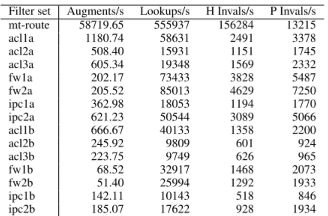
Filter set Augments/s Lookups/s H Invals/s P Invals/s mt-route 58719.65 555937 156284 13215 acl1a 1180.74 58631 2491 3378 acl2a 508.40 15931 1151 1745 acl3a 605.34 19348 1569 2332 fw1a 202.17 73433 3828 5487 fw2a 205.52 85013 4629 7250 ipc1a 362.98 18053 1194 1770 ipc2a 621.23 50544 3089 5066 acl1b 666.67 40133 1358 2200 acl2b 245.92 9809 601 924 acl3b 223.75 9749 626 965 fw1b 68.52 32917 1468 2073 fw2b 51.40 25994 1292 1933 ipc1b 142.11 10143 518 846 ipc2b 185.07 17622 928 1934
Table 2: Maple augments/invalids rates. H Invals and P Invals denote host and port invalidations respectively.
install new rules. During subsequent passes, we measure lookup throughput, as the trace tree has cached results for every packet in the trace. Finally, we perform invalidations for either all hosts used in the trace or for all ports used in the trace
Server: We run Maple on a Dell PowerEdge R210 II server, with 16GB DDR3 memory and Intel Xeon E31270 CPUs (with hyper-threading) running at 3.40GHz. Each CPU has 256KB L2 cache and 8MB shared L3 cache. We run CBench on a separate server and both servers are connected by a 10Gbps Ethernet network.
Results: Table 2 shows throughput for each operation type and policy, using a single 3.40 GHz core, with a single thread. For the
mt-routepolicy, which uses onlyVnodes, Maple can perform all operations at high-speed, including both augments and invali-dates. The augmentation throughput of Classbench-based policies varies. Thefw2bpolicy takes the longest time (20 ms) for Maple to handle a miss. For most policies, invalidation can be handled faster than augmentation, reflecting the fact that invalidations do not require adjusting priority levels, and thus can be done faster.
6.4
Run-time Scheduler
We next evaluate the performance of our multicore scheduler. In particular, if the programmer-provided functionfhas no locality, then all requests will be forwarded to the controller for centralized processing. We use learning switch with exact match to evaluate our scheduler, since this controller is available in other frameworks. We measure both throughput (i.e., the number of requests that our controller can process each second) and latency. The optimizer component of Maple is not executed in evaluations in this sectionto compare with Beacon and NOX-MT [21], two well-known Open-flow control frameworks that aim to provide high performance.
Server: We run our Openflow controllers on an 80 core SuperMi-cro server, with 8 Intel Xeon E7-8850 2.00GHz processors, each having 10 cores with a 24MB smart cache and 32MB L3 cache. We use four 10 Gbps Intel NICs. Our server software includes Linux kernel version 3.7.1 and Intel ixgbe driver (version 3.9.17).
Workload: We simulate switches with a version of Cbench modi-fied to run on several servers, in order to generate sufficient work-load. We use 8 Cbench workload servers connected over 10Gbps links to a single L2 switch, which connects to four 10Gbps inter-faces of our control server. We limit the packet-in messages gener-ated by CBench, so that the number of requests outstanding from a single CBench instance does not exceed a configurable limit. This allows us to control the response time while evaluating throughput.
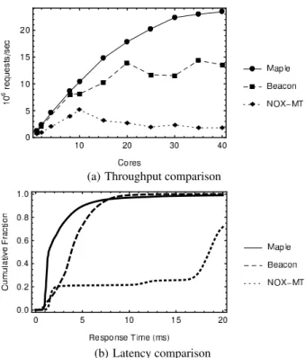
Results: Figure 7(a) shows the throughput as a function of the number of cores used for all three systems. We observe that Maple serves over 20 million requests per second using 40 cores and scales substantially better than Beacon or NOX-MT. In particular Beacon
(a) Throughput comparison
(b) Latency comparison
Figure 7: Throughput and latency of SDN controllers.
scales to less than 15 millions/second, and NOX-MT is only around 2 millions/second. Figure 7(b) shows the corresponding latency CDF for all three systems. The median latency of Maple is 1 ms, Beacon is almost 4 ms, and NOX-MT reaches as high as 17 ms. The95-percentile latency of Maple is still under10ms.
7.
RELATED WORK
SDNs have motivated much recent work, which we classify into basic SDN controllers, programming abstractions, offloading work to switches, and controller scalability.
Basic SDN controllers: NOX [8] offers C++ and Python APIs for raw event handling and switch control, while Beacon [1] offers a similar API for Java. These APIs require the programmer to man-age low-level Openflow state explicitly, such as switch-level rule patterns, priorities, and timeouts. Maple derives this low-level state from a high-level algorithmic policy expression.
SDN programming abstractions and languages: Maestro [3] raises the abstraction level of SDN programming with modular network state management using programmer-defined views. SNAC [19] and FML [9] offer high-level pattern languages for specifying se-curity policies. Onix [10] introduces the NIB abstraction so that applications modify flow tables through reading and writing to the key-value pairs stored in the NIB. Casadoet al.[4] proposes net-work virtualization abstraction. Frenetic [7], Pyretic [16] and Net-tle [23] provide new languages for SDN programming. Frenetic’s NetCore language supports specialized forms of composition, such as between statistics-gathering and control rules. In contrast, Maple is agnostic to the language for expressing policies, and benefits from whatever features (e.g., composition) the language offers.
Offloading work to switches: Devoflow [6] increases scalability by refactoring the Openflow API, reducing the coupling between centralized control