Forecasting with Global Vector Autoregressive Models: A Bayesian Approach

(1)

ePub

WU

Institutional Repository

Jesus Crespo Cuaresma and Martin Feldkircher and Florian Huber

Forecasting with Global Vector Autoregressive Models: A Bayesian Approach

Article (Accepted for Publication) (Refereed)

Original Citation:

Crespo Cuaresma, Jesus and Feldkircher, Martin and Huber, Florian (2016) Forecasting with Global

Vector Autoregressive Models: A Bayesian Approach. Journal of Applied Econometrics, 31 (7). pp.

1371-1391. ISSN 1099-1255

This version is available at: http://epub.wu.ac.at/4701/

Available in ePubWU: August 2017

ePubWU, the institutional repository of the WU Vienna University of Economics and Business, is

provided by the University Library and the IT-Services. The aim is to enable open access to the scholarly output of the WU.

This document is the version accepted for publication and — in case of peer review — incorporates referee comments.

(2)

Forecasting with Global Vector Autoregressive

Models: A Bayesian Approach

∗

Jes´us Crespo Cuaresmaa,b,c,d, Martin Feldkirchere, and Florian Hubere

a_{Vienna University of Economics and Business (WU)} b_{Wittgenstein Centre for Demography and Human Capital (WIC)}

c_{International Institute for Applied Systems Analysis (IIASA)} d_{Austrian Institute of Economic Research (WIFO)}

e_{Oesterreichische Nationalbank (OeNB)}

Abstract

This paper develops a Bayesian variant of global vector autoregressive (B-GVAR) models to forecast an international set of macroeconomic and financial variables. We propose a set of hierarchical priors and compare the predictive performance of B-GVAR models in terms of point and density forecasts for one-quarter-ahead and four-quarters-ahead forecast horizons. We find that forecasts can be improved by employing a global framework and hierarchical priors which induce country-specific degrees of shrinkage on the coefficients of the GVAR model. Forecasts from various B-GVAR specifications tend to outperform forecasts from a naive univariate model, a global model without shrinkage on the parameters and country-specific vector autoregressions.

JEL Classification: C11, C32, C53, C55, F44.

Keywords: International forecasts, shrinkage priors, GVAR.

∗

The opinions expressed in this paper are those of the authors and do not necessarily reflect the official viewpoint of the OeNB or of the Eurosystem. We would like to thank two anonymous referees, Jonas Dovern, Domenico Giannone, Sylvia Fr¨uhwirth-Schnatter, Luca Onorante, Blazej Mazur, M. Hashem Pesaran, Philipp Piribauer and the participants of the 8th _{ECB Workshop on Forecasting Techniques, Frankfurt, the first}

annual conference of the International Association for Applied Econometrics, Queen Mary University, London, the annual meeting of the Austrian Economic Association (NOeG) and internal research seminars at the Vienna University of Economics and Business and the OeNB for helpful comments. Email: [email protected],

(3)

1 Introduction

The rise in international trade and cross-border financial flows in recent decades implies that countries are more than ever exposed to economic shocks from abroad, as demonstrated by the recent global financial crisis. Hence, macroeconomic tools that treat countries as isolated from the rest of the world may miss important information for forecasting and counterfactual analysis. Such concerns do not arise with global vector autoregressive (GVAR) models, as they accommodate spillovers from the global economy in a systematic and transparent manner. The GVAR framework consists of single-country models that are stacked to yield a comprehensive representation of the world economy.

The empirical literature on GVAR models has been largely influenced by the work of

M. Hashem Pesaran and co-authors (Pesaran et al., 2004; Garrat et al., 2006; Dees et al.,

2007b;a). In a series of papers, these authors examine the effect of US macroeconomic shocks on selected foreign economies employing either generalized impulse response functions, struc-tural identification schemes or overidentifying restrictions on long-run relationships between

macroeconomic variables to identify the shocks (Pesaran et al., 2004; Dees et al., 2007b;a).

Recent papers have advanced the literature on GVAR modeling in terms of country

cover-age (Feldkircher,2015), identification of shocks (Eickmeier & Ng,2015) and the specification

of international linkages (Chudik & Fratzscher, 2011; Eickmeier & Ng, 2015; Feldkircher &

Huber,2015;Galesi & Sgherri,2013).

Most of the existing applications of GVAR models concentrate on the quantitative as-sessment of the propagation of macroeconomic shocks using historical data, while very few contributions have addressed their forecasting performance. Evaluating GVAR forecasts in

an out-of-sample exercise, Pesaran et al.(2009) propose to pool GVAR forecasts over

differ-ent estimation windows and model specifications in order to account for potdiffer-ential structural

breaks and misspecifications. Pesaran et al. (2009) conclude that taking global links across

economies into account using GVAR models leads to more accurate out-of-sample predictions than using forecasts based on univariate specifications for output and inflation. Yet for inter-est rates, the exchange rate and financial variables, the results are less spectacular, and the authors also find strong cross-country heterogeneity in the performance of GVAR forecasts.

Employing a GVAR model to forecast macroeconomic variables in five Asian economies,Han

& Ng(2011) find that one-step-ahead forecasts from GVAR models outperform those of stand-alone VAR specifications for short-term interest rates and real equity prices. Concentrating on predicted directional changes to evaluate the forecasting performance of GVAR

specifica-tions, Greenwood-Nimmo et al. (2012) confirm the superiority of GVAR specifications over

univariate benchmark models at long-run forecast horizons.

As an alternative to the GVAR framework a related strand of the literature advocates the estimation of large VARs or panel VARs using Bayesian techniques. More specifically,

(4)

Ba´nburaet al.(2010) assess the forecasting performance of a large-scale monetary VAR based on more than 100 macroeconomic variables and sectoral information. They show that forecasts of these large-scale models can outperform small benchmark VARs when the degree of

shrink-age on the parameters is set accordingly. Giannone & Reichlin(2009) and Alessi & Ba´nbura

(2009) propose to exploit these shrinkage properties and estimate Bayesian VARs with a large

cross-section of countries. Alessi & Ba´nbura(2009) show that Bayesian VAR specifications as

well as dynamic factor models are able to yield accurate one-quarter to four-quarters-ahead

forecasts for international macroeconomic data. Koop & Korobilis (2014) propose a panel

VAR framework that overcomes the problem of overparametrization by averaging over differ-ent restrictions on interdependencies between and heterogeneities across cross-sectional units.

More recently,Korobilis(2015) advocate a particular class of priors that allows for soft

clus-tering of variables or countries, arguing that classical shrinkage priors are inappropriate for panel VARs.

In this contribution, we propose using established shrinkage priors and develop a Bayesian

GVAR (B-GVAR) model. Akin to the GVAR framework, we assume that links among

economies are determined exogenously, while we borrow strength from the Bayesian liter-ature in estimating the individual country models. This allows us to keep the virtues of the GVAR framework with regard to offering a coherent way for policy and counterfactual analysis. Our model includes standard variables that are often employed in small-country VARs such as output, inflation, short-term and long-term interest rates, the real exchange

rate, equity prices and the oil price as a global control variable (see e.g.,Deeset al.,2007b;a;

Pesaran et al.,2004; 2009, among others). This set of variables is extended to feature total credit (domestic and cross-border credit), which can act as an important transmission channel of international shocks.

We compare forecasts of the B-GVAR model under prior specifications that resurface

fre-quently in Bayesian VAR empirical studies: the conjugate Minnesota prior (Litterman,1986)

and its non-conjugate version, and a weighted average of a Minnesota type prior, the “initial dummy observation” prior, which accommodates potential cointegration relationships among the variables considered, and the “single unit root” prior, which facilitates soft-differencing (Doanet al.,1984;Sims,1992;Sims & Zha,1998). We extend this set of random-walk priors

to include the stochastic search variable selection (SSVS) prior proposed by George et al.

(2008) for VAR models. Since the hyperparameters for all priors are elicited locally (i.e.,

for the country model), our approach induces country-specific degrees of shrinkage on the parameters, which is expected to improve forecasts significantly. By inheriting the properties of their single-country VAR counterparts, B-GVAR models are expected to be less prone to

overfitting (Giannone & Reichlin,2009) and allow the researcher to include prior beliefs in the

model, while still taking the long-run co-movement of variables into account. We compare our battery of priors using an expanding window to forecast developments one-quarter-ahead and

(5)

four-quarters-ahead. These forecasts are benchmarked to forecasts of a fifth-order autoregres-sive model with drift term by means of root mean squared errors for point forecasts, and log predictive scores for density forecasts. As another competitor, and to assess the importance of international linkages for forecasting, we evaluate forecasts from isolated, country-specific Bayesian vector autoregressions.

Our analysis provides new insights to the specification and estimation of global macroeco-nomic models. First, we find that forecasts can be improved by employing a global framework that allows for country-specific degrees of shrinkage on the parameters. The proposed Bayesian specifications of the GVAR tend to improve upon forecasts from the naive model, a global model without shrinkage and a shrinkage model that neglects international linkages. Second,

we find that the prior specification put forward in Sims & Zha (1998), the non-conjugate

Minnesota prior and the SSVS prior all show a strong forecasting performance. Third, our analysis indicates that Latin American variables are particularly hard to forecast, while the forecast performance for developed economies is more homogeneous among the specifications considered.

The paper is structured as follows. Section 2 provides a brief description of the global

VAR model, while Section 3 derives its Bayesian variant. In Section 4 we present the data

and perform the forecast evaluation exercise. Finally,Section 5concludes.

2 The GVAR Model

GVAR specifications constitute a compact representation of the world economy designed to model multilateral dependencies among economies across the globe. Basically, a GVAR model consists of a number of country-specific specifications that are combined to form a global model.

The first step is to estimate separate multivariate time series models. In our case, these are standard vector autoregressive models involving a set of endogenous variables and enlarged by weakly exogenous and global control variables (VARX* model). Assuming that our global

economy consists of N + 1 countries, we estimate a VARX* of the following form for every

countryi= 0, ..., N, xit=ai0+ p X s=1 Φisxit−s+ p∗ X r=0 Λirx∗it−r+εit, (2.1)

where xit is a ki ×1 vector of endogenous variables in country i at time t ∈ 1, ..., T, ai0 is

a ki-dimensional vector of intercept terms, Φis (s = 1, . . . , p) denotes the ki ×ki matrix of

parameters associated with the lagged endogenous variables and Λir (r = 1, . . . , p∗) are the

(6)

Furthermore,εit is the standard zero-mean vector error term with variance-covariance matrix

Σεi.

The weakly exogenous or foreign variables, x∗_it, are constructed as a weighted average of

their cross-country counterparts,

x∗_it= N

X

j=0

ωijxjt, (2.2)

withωijdenoting the (non-negative) weight corresponding to the pair of countryiand country

j. We assume thatωii= 0 and PNj=0ωij = 1. The weightsωij reflect economic and financial

ties among economies, which are usually approximated using data on (standardized) bilateral

trade flows.1 The assumption that the x∗_it variables are weakly exogenous at the individual

level reflects the belief that most countries are small relative to the world economy.

Following Pesaran et al. (2004) we stack the N + 1 country-specific models to obtain a

global model, which is given by

Gxt=a0+

Q

X

q=1

Hqxt−q+t. (2.3)

Here, G is a k×k-dimensional matrix that establishes contemporaneous relations between

countries, withk =PN

i=0ki. Furthermore, let a0 be a k-dimensional vector associated with

the constant and Hq(q = 1, . . . , Q) is a k ×k-dimensional global coefficient matrix (with

Q = max(p, p∗)). The matrices G, a0 and Hq are complex functions of the corresponding

country-specific parameters and the bilateral weights. Finally,t is a global vector error term

with variance-covariance matrix Σ. Further details on the derivation of the GVAR model

can be found in AppendixB.

3 The B-GVAR: Priors over Parameters

Bayesian analysis of the GVAR model requires the elicitation of prior distributions for all parameters of the model. We use several prior structures that have been developed for VAR specifications over the parameters of the individual country-specific models, which we extend

to account for the presence of (weakly) exogenous variables.2 For prior implementation, it

proves convenient to rewrite the model in (2.1) as

xit= Π0iZit−1+εit, (3.1)

1_{See e.g.,}_{Eickmeier & Ng}_{(2015) and}_{Feldkircher & Huber}_{(2015) for an application using a broad set of}

different weights.

(7)

where Zit−1 = (1, x0it−1, . . . , x0it−p, x∗

0

it, . . . , x∗

0

it−p∗)0 is of dimension K_i ×1, where K_i = 1 +

kip+k∗i(p∗+ 1) and Πi= (ai0,Φi1, . . . ,Φip,Λi0, . . . ,Λip∗)0 denotes aK_i×k_i matrix of stacked

coefficients. Up to this point we have not adopted any distributional assumptions forεit. We

complete the model specification by assuming that the errors εit are multivariate Gaussian,

i.e.,εit∼ N(0,Σεi).

Rewriting the model in terms of full-data matrices yields

xi =ZiΠi+εi (3.2)

wherexi is a T×ki matrix of stacked endogenous variables,Zi is aT×Ki matrix of stacked

explanatory variables andεi is aT×kimatrix of errors. Furthermore, let Ψi = vec(Πi) denote

thevi-dimensional coefficient vector withvi =kiKi.

The General Conjugate Prior Setup

We start with the simplest prior for the coefficients of the country-specific VARX* models,

which is the natural conjugate prior. In the VARX* framework, we impose an inverted

Wishart prior on Σεi and a multivariate Gaussian prior on Ψi

Ψi|Σεi ∼ N(Ψi,Σεi⊗Vi), (3.3)

Σεi ∼ IW(Si, vi), (3.4)

where Ψ_i andV_i denote prior mean and variance, respectively. Additionally, we letS_i denote

the prior scale matrix andv_ithe prior degrees of freedom for Σεi. The natural conjugate prior

possesses two convenient properties. First, the prior dependence between Ψi and Σεi allows

us to exploit a Kronecker factorization of the likelihood, which translates into significant com-putational advantages. However, it is worth noting that the Kronecker factorization implies prior variances on the coefficients that are proportional across equations of the country model, which might be very restrictive. Second, analytical results for the marginal posterior distri-butions (and functions thereof) are readily available. Especially for forecasting applications where the model has to be re-estimated several times over a training sample, this proves to be a significant advantage.

Following the literature on Bayesian VARs (Litterman, 1986; Sims, 1992; Sims & Zha,

1998), the most common choices for Ψ_iand V_i are given by the so-called random walk priors.

Under the prior, the variables in the system are assumed to follow simple random walks. To implement this prior, we set the prior mean according to

Ψ_ij =

  

a_ij for the first own lag of endogenous variable j in equation j

0 in all other cases.

(8)

wherea_ij (j= 1, . . . , ki) refers to the prior mean over the parameter associated with the first

own lag of theki endogenous variables. Usually these are set to one for variables in levels,

leading to the traditional random walk prior. The assumption that the endogenous variables a priori follow random walk processes at the local level directly carries over to the global model. To see this, note that under the prior model, the coefficients associated with the contemporaneous and lagged (weakly) exogenous variables are set equal to zero. Moreover, the coefficients corresponding to higher lag orders of the endogenous variables are also set

equal to zero. Hence, theGandH matrices reduce to k×kidentity matrices. Consequently,

the global prior model is given by

xt=xt−1+et, (3.6)

where it is straightforward to show that the variance-covariance matrix ofetis a block-diagonal

matrix with the correspondingith block being equal to the prior expectation of Σεi. The only

assumption which is crucial for this result to hold is that the prior mean of coefficients related to the weakly exogenous variables is set to zero.

Several choices are recommended in the literature for the elicitation ofV_i, which translate

into different assumptions about the behavior of the prior model. Doanet al.(1984),Kadiyala

& Karlsson (1997) and Sims & Zha(1998) propose three prominent prior specifications that have been frequently employed by practitioners. The most prominent prior is the Minnesota prior, which has a proven track record in terms of forecasting performance. The Minnesota

prior specifies the prior variance on the coefficients,V_i, such that

V_ig,l=          αi1 rκ_σ

ig for variance on therth lag of coefficient attached to variable g

αi2

(1+r)κ_σ∗

ig for variance on the rth lag of coefficient attached to weakly exog. variable g

αi3 for variances on the deterministic part of the model.

(3.7)

Here, hyperparameters αi1 and αi2 control the tightness of the prior on the endogenous and

weakly exogenous part, respectively. Moreover, the priors are scaled using standard deviations

obtained by running univariate autoregressions on the particular variables. Specifically, σig

refers to the standard deviation of a univariate autoregressive model for the corresponding

variable, whereasσ∗_ig denotes the standard deviation obtained from an autoregressive model

of thelth weakly exogenous variable. Finally,rκ is a deterministic function of the lag length.

Consequently, the strength of the prior belief in the random walk specification is governed

byα1. The hyperparameterκ increasingly tightens the variance on the prior for distant lags,

reflecting the belief that specifications including non-zero parameters associated to variables with long lags tend to have a detrimental effect on the forecasting performance of the model.

(9)

There is a direct link between the locally specified V_i and the global specification of the GVAR model. It is straightforward to show that there exists a relationship between the prior variances on the weakly exogenous variables and the variances related to other countries’ endogenous variables (termed global prior variances). As an illustration, consider

β_in₁, the coefficient associated with the first lag of the nth weakly exogenous variable, i.e.,

xn_it∗ = PN

j=0ωijxnjt, with prior variance given by σ2in. Then, βin1,j = ωijβni1 denotes country

i’s coefficient corresponding to the nth variable of country j with (prior) variance given by

ω2_ijσ2_in. Hence, the corresponding global prior variance is simply scaled down by the trade

links between countriesiand j.3

The Minnesota prior can be implemented by means of so-called dummy observations.

FollowingBa´nbura et al.(2010) andKoop (2013), the moments of the conjugate Minnesota

prior can be matched attaching the following set of artificial dummy observations to the actual data xMi =                01×ki . . . . diag(a_i₁σi1, . . . , aikiσiki)/αi1 0ki(p−1)×ki . . . . 0k∗ i(p∗+1)×ki . . . . diag(σi1, . . . , σiki)                , ZMi =              1 α3 01×(Ki−1) . . . . 0kip×1 Jp⊗diag(σi1, . . . , σiki)/α1 0kip×(Ki−kip−1) . . . . 0(k∗ i(p∗+1))×(kip+1) Jp∗⊗diag(σ ∗ i1, . . . , σ ∗ ik∗ i)/αi2 . . . . 0ki×Ki              , (3.8)

whereJp = diag(1,2, ..., p) andJp∗= diag(1,2, ..., p+ 1). Additionally, 0nq denotes an n×q

dimensional matrix consisting exclusively of zeros.

The first block of x_i and Z_i implements the prior on the deterministic part of the model

whereas the second block implements the random walk prior. Finally, the last two blocks

implement the priors on the weakly exogenous variables and Σεi, respectively.

Second, we consider the “sum-of-coefficients” prior, which softly forces the posterior dis-tribution towards a specification in first differences. This implies that coefficients associated with own, lagged variables in each equation should sum to unity while other coefficients are being pushed towards zero. Implementation of this prior is straightforward by adding the following set of dummy observations to the data

xS_i =diag(a_i₁µ i1, . . . , aikiµiki)/θi1, ZS_i =0ki×1 ι1×p⊗diag(ai1µ_i₁, . . . , aikiµiki)/θi1 0ki×(k ∗ i(p∗+1)) , (3.9)

where µ_ij (j = 1, . . . , ki) denotes the pre-sample mean of the endogenous variables usually

calculated by using the firstpobservations,ι1×p is ap-dimensional row vector of ones andθi1

is a country-specific hyperparameter controlling the tightness of the prior.

(10)

The fact that this prior is not consistent with cointegration gives rise to the “dummy-initial-observation” prior. This prior pushes variables in a country-specific VAR towards their unconditional (stationary) mean, or toward a situation where there is at least one unit root present. That is, either the process has a unit root, or it is stationary and starts near its

mean, implying a penalty for models with inherent initial transient dynamics (Sims, 1992).

Implementation boils down to attaching the following set of dummy observations to the actual data. xI_i =(µi1,...,µiki) θi2 , ZI_i =₀ _ι₁_×_p_⊗(µi1,...,µiki) θi2 ι1×p ∗⊗ (µ∗ i1,...,µ ∗ iki) θi2 . (3.10)

µ∗_ij (j = 1, . . . , k∗_i) denote pre-sample averages from the weakly exogenous variables and θi2

is a hyperparameter controlling the tightness of the dummy-initial-observation prior.

In practice, macroeconomists usually incorporate all three versions of the random walk prior, which can be implemented in a straightforward fashion by combining the three pairs of

dummy observations given in equations (3.8) to (3.10). The final prior, as motivated inSims

& Zha(1998), is then simply a weighted average of the three individual priors described above, where the weights attached to each prior are determined by the associated hyperparameters.

Several studies have emphasized the usefulness of such a weighted prior structure (Ba´nbura

et al.,2010;Giannoneet al.,2013).

Natural conjugate priors require prior dependence between Σεi and Ψi. The traditional

implementation of the Minnesota prior drops this dependence, which provides more flexibility

in terms of prior elicitation. In the empirical application insubsection 4.3 we also consider a

non-conjugate variant of the Minnesota prior. This prior simply replaces the posterior of Σεi

by a known estimate ˆΣεi which leads to analytical posterior solutions.

Stochastic Search Variable Selection (SSVS) Prior

The conjugate priors discussed above apply by definition the same degree of shrinkage across equations. It might be appealing to provide more flexibility in the specification of the prior variance-covariance matrix on the coefficients and move away from the random walk prior model.

The SSVS prior, put forward byGeorge & McCulloch(1993) and subsequently introduced

to the VAR literature byGeorgeet al. (2008), imposes a mixture of Normal distributions on

each coefficient of the VARX*

Ψij|δij ∼(1−δij)N(0, τ02j) +δijN(Ψij, τ12j). (3.11)

Here, Ψ_ij denotes the prior mean and δij is a binary random variable corresponding to

(11)

model and zero if it is a priori excluded from the respective country model. The Normal

distribution corresponding toδij = 0 is typically specified withτ02j close to zero, which pushes

the respective coefficient towards zero. The prior variance of the Normal distribution for

δij = 1,τ12j, is set to a comparatively large value implying a relatively uninformative prior on

coefficient j conditional on inclusion. Note that, in contrast to the Minnesota prior, where

the prior variance on the coefficients differs between different types of variables, the SSVS prior effectively applies an individual degree of shrinkage to every coefficient at the country

level. The SSVS prior has been recently applied within a GVAR framework inFeldkircher &

Huber(2015) to examine the international dimension of US economic shocks.

Defining a scalar parameter dij such that

dij =    τ0j ifδij = 1 τ1j ifδij = 0 (3.12)

and collecting alldij (j= 1, ..., vi) in a vi×vi matrixDi = diag(di1, . . . , divi) the prior on Ψi

simply reduces to the following hierarchical prior setup

Ψi|Di∼ N(Ψi, Ri), (3.13)

Σεi∼ IW(Si, vi), (3.14)

where Ψ_i equals a prior mean matrix, R_i =DiDi and the prior on Σεi is a standard inverse

Wishart prior with prior degrees of freedom given by v_i and prior scale matrix S_i. Note

that the lack of prior dependence between Σεi and Ψi renders this prior (even conditionally)

non-conjugate.

Finally, we followGeorge et al. (2008) and impose a Bernoulli prior on δij

δij ∼Bernoulli(q_ij), (3.15)

whereq

ij denotes the prior inclusion probability of variable j in countryi.

Estimation of this model requires Markov Chain Monte Carlo (MCMC) methods, although

the conditional posteriors of δij,Ψi and Σεi are known. This implies that we can employ a

simplified version of the Gibbs sampler outlined inGeorgeet al.(2008), where we start drawing

Ψi from its full conditional posterior, which follows a Normal distribution. In the next step,

we draw the latent variable δij from a Bernoulli distribution and in the last step we draw

Σεi from an inverse Wishart distribution.4 This algorithm is repeated ntimes and the first

nburn draws are discarded as burn-ins. Averaging the draws ofδij leads to posterior inclusion

probabilities for each variablej. Further details are provided in Appendix D.

4

In contrast to the implementation inGeorgeet al.(2008), we impose an inverse Wishart prior on Σεiand

(12)

4 Empirical Results

4.1 Data and Model Specification

The bulk of the empirical literature employing GVARs use the dataset put forward in Dees

et al.(2007b,a), which covers the most important economies in terms of real activity. For this dataset, time series are available from the early 1980s onward. Other studies have extended the country coverage to feature more emerging economies, at the price of limiting the available

time span (Feldkircher,2015;Feldkircher & Huber,2015). In this paper, our aim is to reserve

a significant share of our available time span for forecast evaluation, which is why we opt to

have rather long time series – at the implied cost of reducing the country coverage.5

We rely on data provided in Dovern et al. (2015), that extend the dataset used in Dees

et al. (2007a,b) with respect to variable coverage and time span. In what follows, we use

quarterly data for 36 countries spanning the period from 1979:Q2 to 2013:Q4.6

The country-specific VARX* models include seven domestic variables. Six variables are

the same as in Dees et al. (2007a,b) and Pesaran et al. (2009), namely real GDP (y), the

change of the consumer price level (∆p), real equity prices (eq), the real exchange rate (e)

vis-´a-vis the US dollar, and short-term (is) and long-term interest rates (il). We enlarge this

set of variables to feature total credit (tc, domestic and cross-border credit), as a seventh

financial variable. This seems to be important, as the hold-out sample for our forecasting exercise contains the global financial crisis, which spread via both the trade and the financial

channel.7 Note that not all variables are available for each of the countries we consider in

this study. With the exception of long-term interest rates, the cross-country coverage of all variables is, however, above 80%. Long-term interest rate data are missing for emerging markets that are characterized by underdeveloped capital markets.

The vector of domestic variables for a typical country iis thus given by

xit= (yit,∆pit, eit, eqit, isit, ilit, tcit)0. (4.1)

We follow the bulk of the literature by including oil prices (poilt) as a global control

vari-able. With the exception of the bilateral real exchange rate, we construct foreign counterparts

5_{Note that this is in contrast to the working paper version of this study available at}_{http://www.oenb.}

at/Publikationen/Volkswirtschaft/Working-Papers/2014/Working-Paper-189.htmlwhich also includes a

forecast comparison to the standard, cointegrated GVAR model put forward inPesaranet al.(2004) andDees

et al.(2007a,b), among others.

6

The following countries are included in the respective regions: Europe includes Austria (AT), Belgium (BE), Germany (DE), Spain (ES), Finland (FI), France (FR), Greece (GR), Italy (IT), Netherlands (ND), Portugal (PT), Denmark (DK), Great Britain (GB), Switzerland (CH), Norway (NO) and Sweden (SE). Other Developed economies feature Australia (AU), Canada (CA), Japan (JP), New Zealand (NZ) and the USA (US). Emerging Asia includes China (CN), India (IN), Indonesia (ID), Malaysia (MY), Korea (KR), Philippines (PH), Singapore (SG) and Thailand (TH). Latin America comprises Argentina (AR), Brazil (BR), Chile (CL), Mexico (MX) and Peru (PE). Mid-East and Africa consists of Turkey (TR), Saudi Arabia (SA) and South Africa (ZA).

(13)

for all domestic variables. The weights to calculate foreign variables are based on average bi-lateral annual trade flows in the period from 1980 to 2003, which denotes the end of our initial

estimation sample.8 For a typical country i the set of weakly exogenous and global control

variables comprises the following variables,

x∗_it= (y∗_it,∆p∗_it, eq_it∗, is∗it, il∗it, tc∗it, poilt∗)0. (4.2)

The US model (i= 0) deviates from the other country specifications in that the oil price

(poilt) is determined within that country model and the trade weighted real exchange rate

(e∗_t) is included to control for co-movements of currencies,

x0t = (y0t,∆p0t, eq0t, is0t, il0t, tc0t, poilt)0, (4.3)

x∗₀_t = (y∗₀_t,∆p∗₀_t, e∗₀_t, eq₀∗_t, is∗0t, il0∗t, tc∗0t)0. (4.4)

The dominant role of the US economy for global financial markets is often accounted for by including a limited set of weakly exogenous variables in its country-specific model. In our setting, coefficients attached to all variables are subject to the shrinkage induced by the priors reviewed in the previous section. It is therefore a priori reasonable to include a large set of international macroeconomic and financial indicators to avoid ad-hoc restrictions, even for a large country such as the US.

For all countries considered, we set the lag length of endogenous and weakly exogenous

variables equal to five. Given the quarterly frequency of the data and the fact that we

introduce Bayesian shrinkage, this seems to be a reasonable choice. We correct for outliers in countries that witnessed extraordinarily strong crisis-induced movements in some of the variables contained in our data. We opted to smooth the relevant time series in these cases rather than include step dummies. While step dummies might control for outliers within the specific country model, extreme shocks might still be carried over to other country models via trade-weighted foreign variables. Obviously, this is not the case when smoothing the series in

the first place.9

8_{Note that recent contributions (Eickmeier & Ng,}_2015;_{Dovern & van Roye,}_{2014) suggest using financial}

data to compute foreign variables related to the financial side of the economy (e.g., interest rates or credit volumes). Since our data sample starts in the early 1980s, reliable data on financial flows – such as portfolio flows or foreign direct investment – are not available. SeeFeldkircher & Huber(2015) for a sensitivity analysis with respect to the choice of weights.

9_{We define outliers as those observations that exceed 1.5 times the interquartile range in absolute value.}

The identified outliers are then smoothed using cubic spline interpolation techniques and in case they are located at the tails of the sample – extrapolation techniques. Using the definition of the interquartile range, we identify 2% of our sample as unusual observations. From these 2%, about 60% regard unusual observations for inflation at the beginning of the observation sample. Short-term interest rates (20%) and the real exchange rate (13%) have historically also shown very volatile patterns for the countries covered in this study. More detailed country-specific information is available from the authors upon request.

(14)

4.2 Selection of Hyperparameters

Due to the strong heterogeneity observed in the world economy, it is daunting to assume that different countries obey the same structural dynamics in terms of macroeconomic fundamen-tals. Thus, using the same set of hyperparameters when eliciting the prior for all countries considered might be too restrictive to unveil differences between economies.

The conjugate priors rely on a set of (presumably fixed) hyperparameters which are ho-mogeneous across countries. A specific set of hyperparameters could, however, induce a tight prior in one country while being relatively loose in other countries. To avoid this problem,

we followCarriero et al.(2015) and choose the hyperparameters by maximizing the marginal

likelihood on a discrete grid of values for α₁ and α₂. For the remaining parameters, we set

α_i₃ = 100 andθi1 =θi2 = 1. For the natural conjugate prior, the marginal likelihood is

avail-able in closed form (see, for instance,Bauwenset al.,2000;Koop,2013). Using the marginal

likelihood as a loss function is motivated by the fact that it can be written as a sequence of one-step-ahead predictive densities. Thus maximizing the marginal likelihood under a flat

prior is equivalent to minimizing the one-step-ahead prediction errors(Geweke,2001;Geweke

& Whiteman, 2006).10 Since the marginal likelihood is not available in closed form for the standard Minnesota prior, we use the hyperparameters obtained from the conjugate prior for

this setting. FollowingCarriero et al. (2015), the parameter controlling the degree of

shrink-age on “other” variables is set equal to 0.8 . Finally, we set a_ij equal to unity for the first

lag of “own” variables except for inflation, where we set a_ij = 0.2. This choice, stipulated in

Clark(2011), is consistent with the notion that all variables are non-stationary.11

For the SSVS prior, we set the prior inclusion probability for each variable equal to 0.5,

which implies that a priori, every variable is assumed equally likely to enter the model. We

set τi,0j = 0.1sij and τi,1j = 10sij and rely on the semi-automatic approach described in

Georgeet al.(2008) to scale the hyperparameters, wheresij is the standard error attached to

coefficient j based on a VARX* estimated by OLS in country i. Finally, we set S_i = 10Iki,

the prior degrees of freedomv_i to ki and Ψi equal to the zero matrix. As a robustness check

we also used a standard random walk prior specification in combination with the SSVS prior. This implies that the prior mean on the first own lag is set equal to unity. However, since

almost no shrinkage is imposed for the case when δij = 1 the results are rather similar with

the standard SSVS implementation. Thus for the sake of brevity we only report the results obtained by setting the prior mean equal to zero for all coefficients. To assess the importance of shrinkage we include in the forecast exercise a prior that is flat over the coefficients (diffuse).

10_{Note that this differs from the procedure proposed by}_Giannone_{et al.}_{(2012), since we do not integrate}

out the hyperparameters in a Bayesian fashion but simply plug in an estimate of the posterior mode ofα1and α₂ under a diffuse prior. This approach seems convenient since it avoids MCMC sampling for the conjugate priors, which proves to be important for the empirical application.

(15)

This prior is implemented by settingα_i₁ =α_i₂=α_i₃= 1010in the conjugate Minnesota prior setup.

4.3 Forecast Performance

The initial estimation period ranges from 1979:Q2 to 2003:Q4 and we use the period 2004:Q1-2013:Q4 as out-of-sample hold-out observations to compare predictive performance across specifications. We base our comparison on recursive one-quarter-ahead and four-quarter-ahead predictions obtained by re-estimating the models over an expanding window defined by the beginning of the available sample and the corresponding period in the hold-out sample. In what follows, we compare the forecast performance for both point and density forecasts. For means of comparison we choose the root mean squared error (RMSE) for point forecasts and

log predictive scores (LPS) to evaluate density forecasts.12 All forecasts are benchmarked to

those of a fifth-order univariate autoregressive (AR(5)) model and forecast errors are reported in an unweighted fashion. That is, we do not attach more weight to favor GVAR specifications that improve forecasts for particular countries which stand out in terms of economic activity. The AR(5) model is estimated in a Bayesian fashion by setting the prior variances of the non-conjugate Minnesota prior such that almost no shrinkage is imposed on the coefficients associated with a given variable while all other coefficients are strongly pushed towards zero.

Forecast Evaluation: Overall Results

Overall results based on one-step-ahead forecasts are provided in the upper panel ofTable 1.

Considering results on point forecasts first, most specifications yield forecasts that improve upon the naive model, as indicated by relative RMSEs below unity.

We start by investigating the relative merits of using shrinkage priors on the one hand, and a global model (without shrinkage on the coefficients) on the other hand. Comparing the results of the BVAR specification with that of the GVAR under a diffuse prior does not yield clear-cut results concerning the superiority of one of the two modelling frameworks for all variables considered. For five out of seven variables, both settings yield on average point forecasts that are more accurate that those of the naive model. Combining the virtues of both approaches (shrinkage and international linkages), however, boosts forecast performance considerably. All B-GVAR prior settings that induce shrinkage outperform the benchmark model. Only one-step-ahead forecasts for inflation under the SSVS prior are similar to those of the benchmark in terms of RMSEs. Comparing B-GVAR shrinkage specifications, our results show a particular good forecast performance for the non-conjugate Minnesota (M-NC) prior

and the prior proposed by Sims & Zha (1998) (S&Z). The non-conjugate Minnesota prior

yields the best point forecasts for four, and the S&Z prior for two out of the seven variables

(16)

considered. The forecast performance of the conjugate variant of the Minnesota prior (M-C) is less spectacular, yielding prediction accuracy measures close to that of the B-GVAR under a diffuse prior setting. Finally, the SSVS framework excels in forecasting total credit, while for the remaining variables forecasts are slightly worse than the ones of the M-NC and S&Z specifications.

Next, we evaluate the relative quality of density forecasts. Table 1, upper panel right-hand

side, displays the sum of log predictive scores over countries per variable, reported as differ-ences to the benchmark autoregressive model. Positive values indicate a better performance of the forecast method under consideration compared to the benchmark. The results confirm the findings for point forecast accuracy. Both isolated country-specific VAR models (BVAR) and the international model without shrinkage (diffuse) outperform forecasts of the naive model. Again, there is no clear superiority structure when comparing these two approaches, while forecasts can be further improved by considering models that explicitly feature inter-national linkages coupled with priors that induce shrinkage on the parameters (M-C, S&Z, M-NC and SSVS). Improvements over forecasts from the benchmark are most pronounced for the SSVS prior and the M-NC specification. The S&Z and M-C priors also yield forecasts gains compared to the benchmark but these are smaller than under the SSVS and M-NC models.

Finally, we consider results based on a four-quarters-ahead forecast horizon. In the

medium-term, forecasts from the naive benchmark specification appear hard to beat. The merits from using shrinkage priors play out more strongly in this setting than in the short-term prediction exercise. While forecasts from the isolated country-specific BVAR models do not tend to worsen markedly with the expanded forecast horizon, the GVAR model under a diffuse prior setting shows a poor forecasting performance. This holds true for both point and density forecasts. In line with our findings on the one-step-ahead forecast horizon, forecasts can be further improved by considering GVAR specifications coupled with shrinkage priors. However, forecast gains are less pronounced than in the short run. Among the prior specifi-cations considered, the S&Z prior excels in point forecast accuracy, while the SSVS and the M-NC prior yield the strongest performance regarding density forecasts.

[Table 1 about here.]

Forecast Evaluation: Cross-Country Differences in Point Forecast Accuracy

In order to examine whether there are systematic cross-country differences in point forecast

accuracy for the priors considered, Figures 1 to 5 show the cross-sectional distribution of

(17)

results for Europe, other developed economies, emerging Asia and Latin America.13 With the exception of Latin America, all plots have the same scaling in order to ease regional comparison of forecast accuracy under the different specifications.

[Figure 1 about here.] [Figure 2 about here.] [Figure 3 about here.] [Figure 4 about here.] [Figure 5 about here.]

The results indicate that point forecast accuracy varies strongly across regions and less so across variables. Taking a regional stance, the largest dispersion of relative RMSE values is observed for variables in Latin American economies. Here the cross-sectional variance of forecast accuracy tends to be large for practically all prior specifications considered. Point forecasts are particularly inaccurate and cross-sectional distributions wide for inflation, total credit and short-term interest rates. For these variables the distributions are about three to four times larger than the ones for the rest of the regions and medians of the distribution of RMSE tend to indicate a worse performance relative to the naive model. Considering the distribution of point forecast accuracy within Latin America, all specifications indicate real exchange rates for Argentina to be particularly hard to forecast. While the dispersion of relative RMSE is markedly smaller in emerging Asia, some of the priors considered yield very inaccurate point forecasts for real activity and inflation in India and Indonesia. By comparison, forecast performance is very homogeneous for variables of European and other developed economies. The distributions of relative predictive ability tend to be very tight, and forecasts that fall far off the median do so for most priors considered. Inaccurate point forecasts for real GDP can be found for Norway, whose economy depends strongly on oil exports, Denmark, Japan and New Zealand. For total credit and the real exchange rate, relative RMSE figures are particularly pronounced in Great Britain and Switzerland, two countries with a large financial sector. Countries that appear as outliers in the box plots might either indicate that some country-specific features (e.g., oil based economy, heavy financial sector) are not correctly reflected in the model, the (linear) specification of the model might be too restrictive or the variance of the underlying time series might be comparably large.

Comparing across prior specifications, these disaggregated results corroborate the findings

provided in Table 1. Concentrating on the median value, most prior specifications tend to

13_{We consider all variables but long-term interest rates and equity prices, for which the cross-country}

coverage is limited. Results for these variables as well as for the four-quarters-ahead forecast horizon are available upon request.

(18)

outperform forecasts from the naive models for all regions and variables with the exception of Latin America. Forecasts under the M-NC, S&Z and SSVS priors often yield the lowest cross-sectional median of relative RMSEs. At first sight, also the diffuse prior yields quite accurate point forecasts. However, the distribution of relative RMSEs tend to be tighter when using priors that incorporate country-specific shrinkage. This holds in particular true for Latin American variables, where relative RMSE distributions under some shrinkage priors are very tight, while the forecast performance indicator is very disperse under the diffuse prior.

5 Conclusions

In this paper we develop a Bayesian GVAR model and assess its out-of-sample predictive performance in terms of point- and density forecasts. We use a large quarterly dataset that starts in 1979:Q2, excels in country coverage and covers many of the most important macroe-conomic and financial variables. This dataset allows us to reserve a significant share of the data as a forecast evaluation sample (40 observations by country, spanning the period from 2004:Q1 to 2013:Q4). Our forecast evaluation sample thus includes periods of very distinct macroeconomic and financial conditions: the period of the great moderation that was accom-panied by stable GDP growth and low inflation, followed by the global financial crisis which triggered most of the economies to enter (prolonged) recession phases, and the ongoing period of recovery since then. Evaluating forecasts over that period yields a fair assessment of the usefulness of Bayesian GVAR models, and the length of our hold-out sample significantly

im-proves upon earlier studies on forecasting using GVAR specifications (see, e.g.,Pesaranet al.,

2009).

Ourmain results are the following. First, we provide ample evidence that taking interna-tional linkages among the economies into account and using priors that induce shrinkage on the parameters locally greatly improves forecast performance. Throughout the set of variables considered in this study, the diffuse prior setup that is flat over the coefficients as well as forecasts from isolated Bayesian VAR models do not tend to rank among the best performing forecast specifications. This holds true for both point forecasts and density forecasts as well as the short-term and medium-term horizon. To set the degree of shrinkage for each country model locally, we numerically optimize the marginal likelihood with respect to the hyperpa-rameters, which is equivalent to minimizing the one-step-ahead prediction errors. This allows us to accommodate a large degree of heterogeneity across the economies, which appears of particular importance for forecasting in a global setting. Second, within the class of Bayesian

GVARs that induce country-specific shrinkage, no single prior dominates all forecasting

se-tups. The S&Z, the non-conjugate version of the Minnesota prior (M-NC) and the SSVS

prior all show a very strong forecast performance over the hold-out sample, while the forecast improvement of the conjugate Minnesota prior compared to the naive benchmark is small.

(19)

The non-conjugate Minnesota prior shows an excellent track record of predictive ability for the one-step-ahead forecast horizon in terms of point forecasts and together with the SSVS prior it excels in short-term density forecasts. The latter also shows a strong density forecast performance in the longer run. The S&Z prior excels in point forecast accuracy and in partic-ular so in the longer run, where its flexibility by that induces shrinkage in various dimensions

(including soft-differencing of the data) seems to pay off. Third,taking a regional stance, our

results indicate that forecasts for Latin America are particularly inaccurate for most specifica-tions considered in this study. By contrast, forecast performance for variables from European or other developed economies is much more homogeneous and differences between the various prior setups considered more modest.

References

Adolfson, M., J.Lind´e, & M.Villani(2007): “Forecasting performance of an open

econ-omy dsge model.” Econometric Reviews 26(2-4): pp. 289–328.

Alessi, L. & M. Ba´nbura (2009): “Comparing global macroeconomic forecasts.” Mimeo. Ba´nbura, M., D. Giannone, & L. Reichlin (2010): “Large bayesian vector auto

regres-sions.” Journal of Applied Econometrics 25(1): pp. 71–92.

Bauwens, L., M.Lubrano, & J.-F.Richard(2000): Bayesian inference in dynamic

econo-metric models. Oxford University Press.

Carriero, A., T. E. Clark, & M. Marcellino (2015): “Bayesian VARs: Specification

Choices and Forecast Accuracy.” Journal of Applied Econometrics 30(1): pp. 46–73.

Chudik, A. & M.Fratzscher(2011): “Identifying the global transmission of the 2007-2009

financial crisis in a GVAR model.” European Economic Review 55(3): pp. 325–339.

Clark, T. E. (2011): “Real-time density forecasts from bayesian vector autoregressions with

stochastic volatility.” Journal of Business & Economic Statistics 29(3).

Dees, S., S. Holly, H. M. Pesaran, & V. L. Smith (2007a): “Long Run Macroeconomic

Relations in the Global Economy.” Economics - The Open-Access, Open-Assessment

E-Journal 1(3): pp. 1–20.

Dees, S., F. di Mauro, H. M. Pesaran, & L. V.Smith (2007b): “Exploring the

interna-tional linkages of the euro area: a global VAR analysis.” Journal of Applied Econometrics

22(1).

Doan, T. R., B. R.Litterman, & C. A.Sims(1984): “Forecasting and Conditional

Projec-tion Using Realistic Prior DistribuProjec-tions.” Econometric Reviews 3: pp. 1–100.

Dovern, J., M. Feldkircher, & F. Huber (2015): “Does Joint Modeling of the World

Economy Pay Off? Evaluating Multivariate Forecasts from a Bayesian GVAR.” Working

Paper Series 200/2015, Oesterreichische Nationalbank.

Dovern, J. & B. van Roye (2014): “International transmission and business-cycle effects

of financial stress.” Journal of Financial Stability 13(0): pp. 1 – 17.

Eickmeier, S. & T.Ng(2015): “How do us credit supply shocks propagate internationally?

a gvar approach.” European Economic Review 74(0): pp. 128 – 145.

Feldkircher, M. (2015): “A Global Macro Model for Emerging Europe.” Journal of

(20)

Feldkircher, M. & F. Huber(2015): “The international transmission of US shocks –

Ev-idence from Bayesian global vector autoregressions.” European Economic Review

forth-coming.

Galesi, A. & S. Sgherri (2013): The GVAR Handbook: Structure and Applications of

a Macro Model of the Global Economy for Policy Analysis, chapter Regional financial spillovers across Europe, pp. 255–270. Oxford University Press.

Garrat, A., K.Lee, M. H.Pesaran, & Y. Shin(2006): Global and National

Macroecono-metric Modelling: A Long-Run Structural Approach. Oxford University Press.

George, E. I. & R.McCulloch (1993): “Variable selection via Gibbs sampling.” Journal

of the American Statistical Association 88: pp. 881–889.

George, E. I., D. Sun, & S.Ni (2008): “Bayesian stochastic search for VAR model

restric-tions.” Journal of Econometrics 142(1): pp. 553–580.

Geweke, J. (2001): “Bayesian econometrics and forecasting.” Journal of Econometrics 100(1): pp. 11–15.

Geweke, J. & G. Amisano (2010): “Comparing and evaluating bayesian predictive

distri-butions of asset returns.” International Journal of Forecasting 26(2): pp. 216–230.

Geweke, J. & C. Whiteman (2006): “Bayesian forecasting.” Handbook of economic

fore-casting 1: pp. 3–80.

Giannone, D., M. Lenza, D. Momferatou, & L. Onorante (2013): “Short-term

infla-tion projecinfla-tions: a Bayesian vector autoregressive approach.” International Journal of

Forecasting .

Giannone, D., M.Lenza, & G. E.Primiceri(2012): “Prior selection for vector

autoregres-sions.” Technical report, National Bureau of Economic Research.

Giannone, D. & L. Reichlin (2009): “Comments on ”Forecasting economic and financial

variables with global VARs”.” International Journal of Forecasting 25(4): pp. 684–686.

Greenwood-Nimmo, M., V. H. Nguyen, & Y. Shin (2012): “Probabilistic Forecasting of

Output Growth, Inflation and the Balance of Trade in a GVAR Framework.” Journal of

Applied Econometrics 27: pp. 554–573.

Han, F. & T. H.Ng(2011): “ASEAN-5 Macroeconomic Forecasting Using a GVAR Model.”

Asian Development Bank, Working Series on Regional Economic Integration 76.

Kadiyala, K. & S.Karlsson(1997): “Numerical Methods for Estimation and Inference in

Bayesian VAR-Models.” Journal of Applied Econometrics 12(2): pp. 99–132.

Karlsson, S. (2012): “Forecasting with Bayesian Vector Autoregressions.”Orebro University¨

Working Paper 12/2012.

Koop, G. & D.Korobilis(2014): “Model uncertainty in panel vector autoregressive models.”

Working Papers 2014-10, Business School - Economics, University of Glasgow.

Koop, G. M. (2013): “Forecasting with medium and large bayesian vars.” Journal of Applied

Econometrics 28(2): pp. 177–203.

Korobilis, D. (2015): “Prior selection for panel vector autoregressions.”MPRA Paper 64143, University Library of Munich.

Litterman, R. (1986): “Forecasting with Bayesian vector autoregressions - Five years of

experience.” Journal of Business and Economic Statistics 5: pp. 25–38.

Pesaran, M. H., T. Schuermann, & L. V. Smith (2009): “Forecasting economic and

financial variables with global VARs.” International Journal of Forecasting 25(4): pp.

642–675.

(21)

Interdepen-dencies Using a Global Error-Correcting Macroeconometric Model.” Journal of Business and Economic Statistics, American Statistical Association 22: pp. 129–162.

Rodgers, D. P. (1985): “Improvements in multiprocessor system design.” In “ACM SIGARCH Computer Architecture News,” volume 13, pp. 225–231. IEEE Computer So-ciety Press.

Sims, C. A. (1992): “Bayesian Inference for Multivariate Time Series with Trend.” presented

at the American statistical Association meetings .

Sims, C. A. & T. Zha(1998): “Bayesian Methods for Dynamic Multivariate Models.”

(22)

T able 1: F orecast p erformance relativ e to autoregressiv e b enc hmark RMSE LPS One-quarter-ahead Conjugate Non-Conjugate Conjugate Non -Con jugate Diffuse M-C S&Z M-NC SSVS BV AR Diffuse M-C S&Z M-NC SSVS BV AR y 0.846 0.900 0.909 0.803 0.883 0.942 135.788 179.872 183.131 136.815 214.057 175.001 ∆ p 1.019 0.911 0.901 0.963 1.000 0.930 9.914 12.053 13.398 14.616 0.157 9.292 e 0.964 0.978 1.002 0.937 0.949 1.009 25.604 35.546 35.563 30.076 26.046 35.373 iS 1.065 0.839 0.778 0.823 0.877 0.833 9.587 4.790 5.665 12.111 5.171 2.207 iL 0.830 0.835 0.837 0.768 0.875 0.863 6.051 6.843 5.850 9.823 -2.194 2.936 eq 0.888 0.857 0.869 0.751 0.826 0.877 270.761 263.597 269.999 270.763 276.233 266.618 tc 1.036 0.969 0.998 0.923 0.915 1.037 61.760 194.628 196.012 120.955 265.352 224.532 F our-quarters-ahead Conjugate Non-Conjugate Conjugate Non -Con jugate Diffuse M-C S&Z M-NC SSVS BV AR Diffuse M-C S&Z M-NC SSVS BV AR y 1.788 0.935 0.865 1.149 1.046 0.895 81.002 135.005 137.740 101.006 150.384 131.648 ∆ p 1.883 1.053 0.977 1.405 1.138 1.025 -13.506 1.549 2.420 -4.614 -12.676 0.241 e 2.234 1.204 1.105 1.723 1.066 1.094 1.802 12.057 15.255 9.611 19.700 17.221 iS 2.090 1.095 0.939 1.308 1.096 0.976 1.015 3.927 4.970 10.646 7.102 0.692 iL 1.864 1.011 0.979 1.163 0.987 0.985 -4.885 5.158 3.897 5.352 -3.578 -0.199 eq 3.080 1.101 1.029 1.831 1.293 0.987 156.659 172.428 173.119 164.492 175.140 170.053 tc 1.235 0.707 0.680 0.881 0.696 0.685 114.907 190.414 194.068 135.085 234.829 212.790 Notes: The figures on the left panel refer to ro ot mean squared erro r (RMSE) relativ e to an autoregressiv e mo del o f order fiv e (AR(5)). V alues b elo w one indicate b etter p erforma nc e of the resp ec tiv e forecast mo del compared to the b enc hmark. F ig ures o n the righ t panel refer to the differences of the sum of v ariable sp ecific log predictiv e scor e s (LP S) re lativ e to the AR(5) b enc hmark. Results based on forecasts o v er the time p erio d 2004:Q1-2013:Q4. Figures for b est p erforming mo dels are in b old. Diffuse stands for the mo del estimated using maxim um lik eliho o d, M-C denotes the GV AR with the conjugate v arian t of the Minnesota prior, S&Z refers to a GV AR estimated using a w ei g h ted a v erage of the conjugate priors as in Sims & Zha ( 1998 ), M-NC stands for the non-conjugate v arian t of the Minnesota prior, SSVS denotes the GV AR estimated using the SSVS prior and BV AR denotes a set of isolated, c o un try-sp ecific v ector autoregressions estimated using the S&Z prior.

(23)

Figure 1: Cross-sectional distribution of 1-step-ahead RMSE values for real GDP (a) Europe ● ● ● ● ● ● ● ● ● 0.6 0.8 1.0 1.2 1.4 GR NO DK NO DK NO NO NO NO Diffuse M−C S&Z M−NC SSVS BV AR

(b) Other developed economies

● ● 0.6 0.8 1.0 1.2 1.4 NZ NZ Diffuse M−C S&Z M−NC SSVS BV AR (c) Emerging Asia ● 0.6 0.8 1.0 1.2 1.4 ID Diffuse M−C S&Z M−NC SSVS BV AR (d) Latin America 0.6 0.8 1.0 1.2 1.4 Diffuse M−C S&Z M−NC SSVS BV AR

Notes:The figures show the cross-sectional distribution of the ratio of the RMSE corresponding to the model to the RMSE of an autoregressive model of order five over the time period 2004:Q1-2013:Q4. Diffuse stands for the model estimated using maximum likelihood, M-C denotes the GVAR with the conjugate variant of the Minnesota prior, S&Z refers to a GVAR estimated using a weighted average of the conjugate priors as in Sims & Zha(1998), M-NC stands for the non-conjugate variant of the Minnesota prior, SSVS denotes the GVAR estimated using the SSVS prior, and BVAR denotes forecasts based on separate country VARs with the S&Z prior employed. Observations that exceed 1.5 times the interquartile range are marked as outliers.

(24)

Figure 2: Cross-sectional distribution of 1-step-ahead RMSE values for inflation (a) Europe ● ● ● 0.6 0.7 0.8 0.9 1.0 1.1 1.2 1.3 SE FR FR Diffuse M−C S&Z M−NC SSVS BV AR

0.6 0.7 0.8 0.9 1.0 1.1 1.2 1.3 Diffuse M−C S&Z M−NC SSVS BV AR (c) Emerging Asia ● ● 0.6 0.7 0.8 0.9 1.0 1.1 1.2 1.3 IN IN Diffuse M−C S&Z M−NC SSVS BV AR (d) Latin America ● 0.5 1.0 1.5 2.0 2.5 3.0 3.5 CL Diffuse M−C S&Z M−NC SSVS BV AR

(25)

Figure 3: Cross-sectional distribution of 1-step-ahead RMSE values for the real exchange rate (a) Europe ● ● ● 0.8 1.0 1.2 1.4 1.6 GB _CH GB Diffuse M−C S&Z M−NC SSVS BV AR

0.8 1.0 1.2 1.4 1.6 Diffuse M−C S&Z M−NC SSVS BV AR (c) Emerging Asia 0.8 1.0 1.2 1.4 1.6 Diffuse M−C S&Z M−NC SSVS BV AR (d) Latin America ● ● ● ● 0.8 1.0 1.2 1.4 1.6 AR CL AR AR Diffuse M−C S&Z M−NC SSVS BV AR

(26)

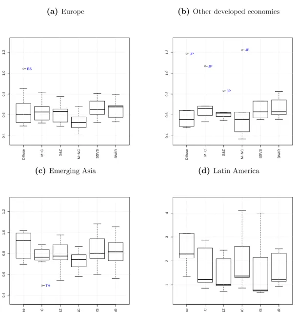
Figure 4: Cross-sectional distribution of 1-step ahead RMSE values for short-term interest rates (a) Europe ● 0.4 0.6 0.8 1.0 1.2 ES Diffuse M−C S&Z M−NC SSVS BV AR

● ● ● ● 0.4 0.6 0.8 1.0 1.2 JP JP JP JP Diffuse M−C S&Z M−NC SSVS BV AR (c) Emerging Asia ● 0.4 0.6 0.8 1.0 1.2 TH Diffuse M−C S&Z M−NC SSVS BV AR (d) Latin America ● 1 2 3 4 AR Diffuse M−C S&Z M−NC SSVS BV AR

(27)

Figure 5: Cross-sectional distribution of 1-step-ahead RMSE values for total credit (a) Europe ● ● 0.6 0.8 1.0 1.2 1.4 1.6 GB CH Diffuse M−C S&Z M−NC SSVS BV AR

0.6 0.8 1.0 1.2 1.4 1.6 Diffuse M−C S&Z M−NC SSVS BV AR (c) Emerging Asia 0.6 0.8 1.0 1.2 1.4 1.6 Diffuse M−C S&Z M−NC SSVS BV AR (d) Latin America 0.5 1.0 1.5 2.0 2.5 3.0 Diffuse M−C S&Z M−NC SSVS BV AR

Notes:The figures show the cross-sectional distribution of the ratio of the RMSE corresponding to the model to the RMSE of an autoregressive model of order five over the time period 2004:Q1-2013:Q4.Diffuse stands for the model estimated using maximum likelihood,M-C denotes the GVAR with the conjugate variant of the Minnesota prior,S&Z refers to a GVAR estimated using a weighted average of the conjugate priors as inSims & Zha(1998),M-NC stands for the non-conjugate variant of the Minnesota prior,SSVS denotes the GVAR estimated using the SSVS prior andBVARdenotes a set of isolated, country-specific vector autoregressions estimated using the S&Z prior. Observations that exceed 1.5 times the interquartile range are marked as outliers.

(28)

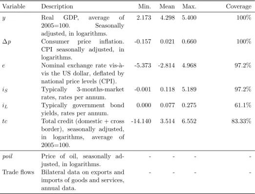
Appendix A Data Description

Table A.1: Data description

Variable Description Min. Mean Max. Coverage

y Real GDP, average of 2005=100. Seasonally adjusted, in logarithms.

2.173 4.298 5.400 100%

∆p Consumer price inflation. CPI seasonally adjusted, in logarithms.

-0.157 0.021 0.660 100%

e Nominal exchange rate vis-` a-vis the US dollar, deflated by national price levels (CPI).

-5.373 -2.814 4.968 97.2%

iS Typically 3-months-market rates, rates per annum.

-0.001 0.118 5.189 97.2%

iL Typically government bond yields, rates per annum.

0.000 0.077 0.275 61.1%

tc Total credit (domestic + cross border), seasonally adjusted, in logarithms, average of 2005=100.

-14.140 3.514 6.552 83.33%

poil Price of oil, seasonally ad-justed, in logarithms.

- - -

-Trade flows Bilateral data on exports and imports of goods and services, annual data.

- - -

-Notes: Summary statistics pooled over countries and time. The coverage refers to the cross-country availability per country, in %. Data are from the IMF’s IFS data base and national sources. Trade flows stem from the IMF’s DOTS data base. For more details see the data appendix inFeldkircher(2015).

Appendix B Deriving the GVAR Model

For the sake of exposition, let us assume thatp= 1, p∗ = 1 and ai0 = 0. Following Pesaran

et al.(2004), the country-specific models in equation (2.1) can be rewritten as

Aizit =Bizit−1+εit, (B.1)

where Ai = (Iki,−Λi0), Bi = (Φi,−Λi1) and zit = (x

0 it, x∗

0

it)0. By defining a suitable link

matrixWi of dimension (ki+ki∗)×k, wherek =

PN

i=0ki, we can rewrite zit as zit =Wixt,

withxt (the so-called global vector) being a vector where all the endogenous variables of the

countries in our sample are stacked, i.e.,xt= (x00t, . . . , x0N t)0. ReplacingzitwithWixtin (B.1)

and stacking the different local models leads yields the global model,

xt = G−1Hxt−1+G−1t

= F xt−1+et. (B.2)

Here, G = ((A0W0)0,· · ·,(ANWN)0)0 and H = ((B0W0)0,· · · ,(BNWN)0)0 denote the

(29)

specifi-cations. In line with existing work (e.g.,Dees et al.,2007b) we assume that G is invertible.

Finally,et∼ N(0,Σe), where Σe=G−1Σ(G−1)0 and Σ is a block-diagonal matrix given by

Σ =      Σε0 0 · · · 0 0 Σε1 · · · 0 .. . ... . .. ... 0 0 · · · ΣεN      . (B.3)

Consequently, the matrix G establishes contemporaneous cross-country correlations. The

eigenvalues of the matrixF provide information about the stability of the global system. In the

empirical application we rule out explosive behavior of the model by discarding posterior draws that significantly fall outside the unit circle. The framework outlined above deviates from the

work pioneered by Pesaran et al. (2004) in that we do not explicitly impose cointegration

relationships in the individual country-specific models.

Appendix C Posterior Distributions The Conjugate Case

For all priors discussed inSection 3that can be cast into a form that uses dummy observations,

prior quantities can be expressed as

Π_i = (Z0_iZ_i)−1Z0_ix_i (C.1)

V_i = (Z0_iZ_i)−1 (C.2)

S_i = (x_i−Z_iΠ_i)0(x_i−Z_iΠ_i) (C.3)

whereZ_i, x_idenotes any (or a combination) of the dummy observations discussed inSection 3.

In the conjugate case, the posterior distributions of Ψi and Σεiare of Normal and

inverse-Wishart form, respectively. Formally, this implies that

Ψi|Σεi,DiT ∼ N(Ψi,Σεi⊗Vi) (C.4)

Σεi|Ψi,DiT ∼ IW(Si, vi) (C.5)

whereD_iT denotes the information set spanned by observations for country iup to time T.

The posterior mean of Ψi = vec(Πi) is given by

Πi = (Z

0

iZi)−1Z 0

ixi, (C.6)

where Zi and xi denote the dummy-observation-augmented data matrices. Moreover, Vi is

simply

Vi= (Z 0

iZi)−1 (C.7)

The scale matrix of the posterior of Σεi is given by

(30)

and the posterior degrees of freedom are T +vi. The conjugate nature of this prior implies that posterior distributions are available in closed-form.

The Non-Conjugate / SSVS Case

FollowingGeorgeet al. (2008), we replace Σεi⊗Vi in equation (C.4) by avi×vi matrixRi,

where

Ri = Σ−_εi1⊗(Zi0Zi) +R−_i1

−1

. (C.9)

The mean of the conditional posterior is given by

Ψi=Ri R−i 1Ψi+ Σ −1 εi ⊗(Z 0 ix 0 i) . (C.10)

The posterior degrees of freedom are stillvi=T+vi and the posterior scale matrix is given

by

Si =Si+ (xi−ZiΠi)0(xi−ZiΠi). (C.11)

Finally, the conditional posterior ofδij is distributed as Bernoulli,

δij|δi•,Ψi,Σεi,DiT ∼Bernoulli(qij) (C.12)

where the notation δi• indicates conditioning on all δig for g 6= j and the probability that

δij = 1 is given by q_ij = 1 τ1jexp(− Ψ2_ij 2τ1j) 1 τ1jexp(− Ψ2 ij 2τ1j)qij+ 1 τ0j exp(− Ψ2 ij 2τ0j)(1−qij) . (C.13)

Appendix D Posterior Inference at the Global Level: The Implications and Ad-vantages of Country-Specific Priors

The method described in Section3imposes priors exclusively at the individual country level.

The main reason for local prior elicitation is computational. Furthermore, it is straightforward to show that placing the priors locally leads to the same priors on the global level scaled by the strength of the invoked trade links.

Prior implications at the global level

The global implications of a prior imposed locally and the corresponding prior variances can

be derived by substitutingWixt in equation (B.1),