arxiv: v3 [cond-mat.str-el] 10 Jun 2014

(1)

A Practical Introduction to Tensor Networks:

Matrix Product States and Projected Entangled Pair States

Rom´

an Or´

us

∗

Institute of Physics, Johannes Gutenberg University, 55099 Mainz,

Germany

June 11, 2014

Abstract

This is a partly non-technical introduction to selected topics on tensor network methods, based on several lectures and introductory seminars given on the subject. It should be a good place for newcomers to get familiarized with some of the key ideas in the field, specially regarding the numerics. After a very general introduction we motivate the concept of tensor network and provide several examples. We then move on to explain some basics about Matrix Product States (MPS) and Projected Entangled Pair States (PEPS). Selected details on some of the associated numerical methods for 1dand 2dquantum lattice systems are also discussed.

∗_{E-mail address:} _{[email protected]}

(2)

Introduction

During the last years, the field of Tensor Networks has lived an explosion of results in several directions. This is specially true in the study of quantum many-body systems, both theoretically and numerically. But also in directions which could not be envisaged some time ago, such as its relation to the holographic principle and the AdS/CFT correspondence in quantum gravity [1,2]. Nowadays, Tensor Networks is rapidly evolving as a field and is embracing an interdisciplinary and motivated community of researchers.

This paper intends to be an introduction to selected topics on the ever-expanding field of Tensor Networks, mostly focusing on some practical (i.e. algorithmic) applications of Matrix Product States and Projected Entangled Pair States. It is mainly based on several introductory seminars and lectures that the author has given on the topic, and the aim is that the unexperienced reader can start getting familiarized with some of the usual concepts in the field. Let us clarify now, though, that we do not plan to cover all the results and techniques in the market, but rather to present some insightful information in a more or less comprehensible way, sometimes also trying to be intuitive, together with further references for the interested reader. In this sense, this paper is not intended to be a complete review on the topic, but rather a useful manual for the beginner. The text is divided into several sections. Sec.2 provides a bit of background on the topic. Sec.3 motivates the use of Tensor Networks, and in Sec.4 we introduce some basics about Tensor Network theory such as contractions, diagrammatic notation, and its relation to quantum many-body wave-functions. In Sec.5we introduce some generalities about Matrix Product States (MPS) for 1d systems and Projected Entangled Pair States (PEPS) for 2d systems. Later in Sec.6 we explain several strategies to compute expectation values and effective environments for MPS and PEPS, both for finite systems as well as systems in the thermodynamic limit. In Sec.7we explain generalities on two families of methods to find ground states, namely variational optimization and imaginary time evolution. Finally, in Sec.8 we provide some final remarks as well as a brief discussion on further topics for the interested reader.

2

A bit of background

Understanding quantum many-body systems is probably the most challenging problem in con-densed matter physics. For instance, the mechanisms behind high-Tc superconductivity are still a

mystery to a great extent despite many efforts [3]. Other important condensed matter phenomena beyond Landau’s paradigm of phase transitions have also proven very difficult to understand, in turn combining with an increasing interest in new and exotic phases of quantum matter. Examples of this are, to name a few, topologically ordered phases (where a pattern of long-range entangle-ment prevades over the whole system) [4], quantum spin liquids (phases of matter that do not break any symmetry) [5], and deconfined quantum criticality (quantum critical points between phases of fundamentally-different symmetries) [6].

The standard approach to understand these systems is based on proposing simplified models that are believed to reproduce the relevant interactions responsible for the observed physics, e.g. the Hubbard andt−Jmodels in the case of high-Tcsuperconductors [7]. Once a model is proposed,

and with the exception of some lucky cases where these models are exactly solvable, one needs to rely on faithful numerical methods to determine their properties.

As far as numerical simulation algorithms are concerned,Tensor Network (TN) methods have become increasingly popular in recent years to simulate strongly correlated systems [8]. In these methods the wave function of the system is described by a network of interconnected tensors. Intuitively, this is like a decomposition in terms of LEGOR _{pieces, and where entanglement plays}

(4)

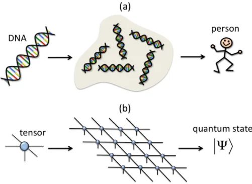
the role of a “glue” amongst the pieces. To put it in another way, the tensor is the DNA of the wave-function, in the sense that the whole wave-function can be reconstructed from this fundamental piece, see Fig.(1). More precisely, TN techniques offer efficient descriptions of quantum many-body states that are based on the entanglement content of the wave function. Mathematically, the amount and structure of entanglement is a consequence of the chosen network pattern and the number of parameters in the tensors.

Figure 1: (color online) (a) The DNA is the fundamental building block of a person. In the same way, (b) the tensor is the fundamental building block of a quantum state (here we use a diagrammatic notation for tensors that will be made more precise later on). Therefore, we could say that the tensor is the DNA of the wave-function, in the sense that the whole wave-function can be reconstructed from it just by following some simple rules.

The most famous example of a TN method is probably the Density Matrix Renormalization Group (DMRG) [9,10,11,12], introduced by Steve White in 1992. One could say that this method has been the technique of reference for the last 20 years to simulate 1dquantum lattice systems. However, many important breakthroughs coming from quantum information science have under-pinned the emergence of many other algorithms based on TNs. It is actually quite easy to get lost in the soup of names of all these methods, e.g. Time-Evolving Block Decimation (TEBD) [13, 14], Folding Algorithms [15], Projected Entangled Pair States (PEPS) [16], Tensor Renor-malization Group (TRG) [18], Tensor-Entanglement Renormalization Group (TERG) [17], Tensor Product Variational Approach [19], Weighted Graph States [20], Entanglement Renormalization (ER) [21], Branching MERA [22], String-Bond States [23], Entangled-Plaquette States [24], Monte Carlo Matrix Product States [25], Tree Tensor Networks [26], Continuous Matrix Product States and Continuous Tensor Networks [27], Time-Dependent Variational Principle (TDVP) [28], Sec-ond Renormalization Group (SRG)[29], Higher Order Tensor Renormalization Group (HOTRG) [30]... and these are just some examples. Each one of these methods has its own advantages and disadvantages, as well as optimal range of applicability.

A nice property of TN methods is their flexibility. For instance, one can study a variety of systems in different dimensions, of finite or infinite size [31, 14, 32, 33, 18, 29, 30, 34], with

(5)

different boundary conditions [11,35], symmetries [36], as well as systems of bosons [37], fermions [38] and frustrated spins [39]. Different types of phase transitions [40] have also been studied in this context. Moreover, these methods are also now finding important applications in the context of quantum chemistry [41] and lattice gauge theories [42], as well as interesting connections to quantum gravity, string theory and the holographic principle [2]. The possibility of developing algorithms for infinite-size systems is quite relevant, because it allows to estimate the properties of a system directly in the thermodynamic limit and without the burden of finite-size scaling effects1_.

Examples of methods using this approach are iDMRG [31] and iTEBD [14] in 1d(the “i” means infinite), as well as iPEPS [32], TRG/SRG [18,29], and HOTRG [30] in 2d. From a mathematical perspective, a number of developments in tensor network theory have also come from the field of low-rank tensor approximations in numerical analysis [43].

3

Why Tensor Networks?

Considering the wide variety of numerical methods for strongly correlated systems that are avail-able, one may wonder about the necessity of TN methods at all. This is a good question, for which there is no unique answer. In what follows we give some of the reasons why these methods are important and, above all, necessary.

3.1

New boundaries for classical simulations

All the existing numerical techniques have their own limitations. To name a few: the exact diago-nalization of the quantum Hamiltonian (e.g. Lanczos methods [44]) is restricted to systems of small size, thus far away from the thermodynamic limit where quantum phase transitions appear. Series expansion techniques [45] rely on perturbation theory calculations. Mean field theory [46] fails to incorporate faithfully the effect of quantum correlations in the system. Quantum Monte Carlo algorithms [47] suffer from the sign problem, which restricts their application to e.g. fermionic and frustrated quantum spin systems. Methods based on Continuous Unitary Transformations [48] rely on the approximate solution of a system of infinitely-many coupled differential equations. Coupled Cluster Methods [49] are restricted to small and medium-sized molecules. And Density Functional Theory [50] depends strongly on the modeling of the exchange and correlation interactions amongst electrons. Of course, these are just some examples.

TN methods are not free from limitations either. But as we shall see, their main limitation is very different: the amount and structure of the entanglement in quantum many-body states. This new limitation in a computational method extends the range of models that can be simulated with a classical computer in new and unprecedented directions.

3.2

New language for (condensed matter) physics

TN methods represent quantum states in terms of networks of interconnected tensors, which in turn capture the relevant entanglement properties of a system. This way of describing quantum states is radically different from the usual approach, where one just gives the coefficients of a wave-function in some given basis. When dealing with a TN state we will see that, instead of thinking about complicated equations, we will be drawingtensor network diagrams, see Fig.(2). As such, it has been recognized that this tensor description offers the natural language to describe quantum states of matter, including those beyond the traditional Landau’s picture such as quantum spin

(6)

liquids and topologically-ordered states. This is a new language for condensed matter physics (and in fact, for all quantum physics) that makes everything much more visual and which brings new intuitions, ideas and results.

Figure 2: (color online) Two examples of tensor network diagrams: (a) Matrix Product State (MPS) for 4 sites with open boundary conditions; (b) Projected Entangled Pair State (PEPS) for a 3×3 lattice with open boundary conditions.

3.3

Entanglement induces geometry

Imagine that you are given a quantum many-body wave-function. Specifying its coefficients in a given local basis does not give any intuition about the structure of the entanglement between its constituents. It is expected that this structure is different depending on the dimensionality of the system: this should be different for 1d systems, 2d systems, and so on. But it should also depend on more subtle issues like the criticality of the state and its correlation length. Yet, naive representations of quantum states do not possess any explicit information about these properties. It is desirable, thus, to find a way of representing quantum sates where this information is explicit and easily accessible.

As we shall see, a TN has this information directly available in its description in terms of a network of quantum correlations. In a way, we can think of TN states as quantum states given in some entanglement representation. Different representations are better suited for different types of states (1d, 2d, critical...), and the network of correlations makes explicit the effective lattice geometry in which the state actually lives. We will be more precise with this in Sec.4.2. At this level this is just a nice property. But in fact, by pushing this idea to the limit and turning it around, a number of works have proposed that geometry and curvature (and hence gravity) could emerge naturally from the pattern of entanglement present in quantum states [51]. Here we will not discuss further this fascinating idea, but let us simply mention that it becomes apparent that the language of TN is, precisely, the correct one to pursue this kind of connection.

3.4

Hilbert space is far too large

This is, probably, the main reason why TNs are a key description of quantum many-body states of Nature. For a system of e.g. N spins 1/2, the dimension of the Hilbert space is 2N_{, which}

is exponentially large in the number of particles. Therefore, representing a quantum state of the many-body system just by giving the coefficients of the wave function in some local basis is an inefficient representation. The Hilbert space of a quantum many-body system is a really big place with an incredibly large number of quantum states. In order to give a quantitative idea, let us put some numbers: ifN ∼1023 _{(of the order of the Avogadro number) then the number of basis}

(7)

Figure 3: (color online) The entanglement entropy between A and B scales like the size of the boundary ∂Abetween the two regions, henceS∼∂A.

states in the Hilbert space is∼O(101023

), which is much larger (in factexponentially larger) than the number of atoms in the observable universe, estimated to be around 1080_{! [}₅₂_]

Luckily enough for us, not all quantum states in the Hilbert space of a many-body system are equal: some are more relevant than others. To be specific, many important Hamiltonians in Nature are such that the interactions between the different particles tend to be local (e.g. nearest or next-to-nearest neighbors)2. And locality of interactions turns out to have important consequences. In particular, one can prove that low-energy eigenstates of gapped Hamiltonians with local interactions obey the so-called area-law for the entanglement entropy [53], see Fig.(3). This means that the entanglement entropy of a region of space tends to scale, for large enough regions, as the size of the boundary of the region and not as the volume3. And this is a very remarkable property, because a quantum state picked at random from a many-body Hilbert space will most likely have a entanglement entropy between subregions that will scale like the volume, and not like the area. In other words, low-energy states of realistic Hamiltonians are not just “any” state in the Hilbert space: they are heavily constrained by locality so that they must obey the entanglement area-law.

By turning around the above consideration, one finds a dramatic consequence: it means that not “any” quantum state in the Hilbert space can be a low-energy state of a gapped, local Hamiltonian. Only those states satisfying the area-law are valid candidates. Yet, the manifold containing these states is just a tiny, exponentially small, corner of the gigantic Hilbert space (see Fig.(4)). This corner is, therefore, thecorner of relevant states. And if we aim to study states within this corner, then we better find a tool to target it directly instead of messing around with the full Hilbert space. Here is where the good news come: it is the family of TN states the one that targets this most relevant corner of states [57]. Moreover, recall that Renormalization Group (RG) methods for many-body systems aim to, precisely, identify and keep track of the relevant degrees of freedom to describe a system. Thus, it looks just natural to devise RG methods that deal with this relevant corner of quantum states, and are therefore based on TN states.

In fact, the consequences of having such an immense Hilbert space are even more dramatic. For instance, one can also prove that by evolving a quantum many-body state a timeO(poly(N)) with a local Hamiltonian, the manifold of states that can be reached in this time is also exponentially small [58]. In other words: the vast majority of the Hilbert space is reachable only after a time evolution that would take O(exp(N)) time. This means that, given some initial quantum state

2_{Here we will not enter into deep reasons behind the locality of interactions, and will simply take it for granted.} Notice, though, that there are also many important condensed-matter Hamiltonians with non-local interactions, e.g., with a long-range Coulomb repulsion.

3_{For gapless Hamiltonians there may be multiplicative and/or additive corrections to this behavior, see e.g. Refs.} [54,55,56].

(8)

Figure 4: (color online) The manifold of quantum states in the Hilbert space that obeys the area-law scaling for the entanglement entropy corresponds to a tiny corner in the overall huge space.

(which quite probably will belong to the relevant corner that satisfies the area-law), most of the Hilbert space isunreachable in practice. To have a better idea of what this means let us put again some numbers: forN ∼1023_{particles, by evolving some quantum state with a local Hamiltonian,}

reaching most of the states in the Hilbert space would take ∼ O(101023_{) seconds. Considering}

that the best current estimate for the age of the universe is around 1017 _{seconds [}₅₉_{], this means}

that we should wait around the exponential of one-million times the age of the universe to reach most of the states available in the Hilbert space. Add to this that your initial state must also be compatible with some locality constraints in your physical system (because otherwise it may not be truly physical), and what you obtain is that all the quantum states of many-body systems that you will ever be able to explore are contained in a exponentially small manifold of the full Hilbert space. This is why the Hilbert space of a quantum many-body systems is sometimes referred to as a convenient illusion [58]: it is convenient from a mathematical perspective, but it is an illusion because no one will ever see most of it.

4

Tensor Network theory

Let us now introduce some mathematical concepts. In what follows we will define what a TN state is, and how this can be described in terms of TN diagrams. We will also introduce the TN representation of quantum states, and explain the examples of Matrix Product States (MPS) for 1dsystems [60], and Projected Entangled Pair States (PEPS) for 2dsystems [16].

4.1

Tensors, tensor networks, and tensor network diagrams

For our purposes, atensor is a multidimensional array of complex numbers. Therank of a tensor is the number of indices. Thus, a rank-0 tensor is scalar (x), a rank-1 tensor is a vector (vα), and

a rank-2 tensor is a matrix (Aαβ).

Anindex contraction is the sum over all the possible values of the repeated indices of a set of tensors. For instance, the matrix product

Cαγ=

D

X

β=1

(9)

is the contraction of index β, which amounts to the sum over itsD possible values. One can also have more complicated contractions, such as this one:

Fγωρσ=

D

X

α,β,δ,ν,µ=1

AαβδσBβγµCδνµωEνρα, (2)

where for simplicity we assumed that contracted indicesα, β, δ, νandµcan takeDdifferent values. As seen in these examples, the contraction of indices produces new tensors, in the same way that e.g. the product of two matrices produces a new matrix. Indices that are not contracted are called open indices.

A Tensor Network (TN) is a set of tensors where some, or all, of its indices are contracted according to some pattern. Contracting the indices of a TN is called, for simplicity, contracting the TN. The above two equations are examples of TN. In Eq.(1), the TN is equivalent to a matrix product, and produces a new matrix with two open indices. In Eq.(2), the TN corresponds to contracting indices α, β, δ, ν and µ in tensors A, B, C and E to produce a new rank-4 tensor F

with open indices γ, ω, ρandσ. In general, the contraction of a TN with some open indices gives as a result another tensor, and in the case of not having any open indices the result is a scalar. This is the case of e.g. the scalar product of two vectors,

C=

D

X

α=1

AαBα , (3)

whereC is a complex number (rank-0 tensor). A more intrincate example could be

F =

D

X

α,β,γ,δ,ω,ν,µ=1

AαβδγBβγµCδνµωEνωα , (4)

where all indices are contracted and the result is again a complex numberF.

Once this point is reached, it is convenient to introduce a diagrammatic notation for tensors and TNs in terms oftensor network diagrams, see Fig.(5). In these diagrams tensors are represented by shapes, and indices in the tensors are represented by lines emerging from the shapes. A TN is thus represented by a set of shapes interconnected by lines. The lines connecting tensors between each other correspond to contracted indices, whereas lines that do not go from one tensor to another correspond to open indices in the TN.

Figure 5: (color online) Tensor network diagrams: (a) scalar, (b) vector, (c) matrix and (d) rank-3 tensor

Using TN diagrams it is much easier to handle calculations with TN. For instance, the contrac-tions in Eqs.(1, 2, 3, 4) can be represented by the diagrams in Fig.(6). Also tricky calculations, like the trace of the product of 6 matrices, can be represented by diagrams as in Fig.(7). From the TN diagram the cyclic property of the trace becomes evident. This is a simple example of why TN

(10)

Figure 6: (color online) Tensor network diagrams for Eqs.(1, 2, 3, 4): (a) matrix product, (b) contraction of 4 tensors with 4 open indices, (c) scalar product of vectors, and (d) contraction of 4 tensors without open indices.

Figure 7: (color online) Trace of the product of 6 matrices.

diagrams are really useful: unlike plain equations, TN diagrams allow to handle with complicated expressions in a visual way. In this manner many properties become apparent, such as the cyclic property of the trace of a matrix product. In fact, you could compare the language of TN diagrams to that of Feynman diagrams in quantum field theory. Surely it is much more intuitive and visual to think in terms of drawings instead of long equations. Hence, from now on we shall only use diagrams to represent tensors and TNs.

There is an important property of TN that we would like to stress now. Namely, that the total number of operations that must be done in order to obtain the final result of a TN contraction depends heavily on the order in which indices in the TN are contracted. See for instance Fig.(8). Both cases correspond to the same overall TN contraction, but in one case the number of operations is O(D4_{) and in the other is}_O₍_D5_{). This is quite relevant, since in TN methods one has to deal}

with many contractions, and the aim is to make these as efficiently as possible. For this, finding the optimal order of indices to be contracted in a TN will turn out to be a crucial step, specially when it comes to programming computer codes to implement the methods. To minimize the computational cost of a TN contraction one must optimize over the different possible orderings of pairwise contractions, and find the optimal case. Mathematically this is a very difficult problem, though in practical cases this can be done usually by simple inspection.

(11)

Figure 8: (color online) (a) Contraction of 3 tensors inO(D4_{) time; (b) contraction of the same 3}

tensors in O(D5_{) time.}

4.2

Breaking the wave-function into small pieces

Let us now explain the TN representation of quantum many-body states. For this, we consider a quantum many-body system ofN particles. The degrees of freedom of each one of these particles can be described by pdifferent states. Hence, we are considering systems of N p-level particles. For instance, for a quantum many-body system such as the spin-1/2 Heisenberg model we have that p= 2, so that each particle is a 2-level system (or qubit). For a given system of this kind, any wave function |Ψithat describes its physical properties can be written as

|Ψi= X

i1i2...iN

Ci1i2...iN|i1i ⊗ |i2i ⊗ · · · ⊗ |iNi (5)

once an individual basis |irifor the states of each particle r= 1, ..., N has been chosen. In the

above equation,Ci1i2...iN arep

N _{complex numbers (independent up to a normalization condition),}

ir= 1, ..., pfor each particler, and the symbol⊗denotes the tensor product of individual quantum

states for each one of the particles in the many-body system.

Notice now that thepN numbersCi1i2...iN that describe the wave function|Ψican be understood

as the coefficients of a tensorCwithN indicesi1i2. . . iN, where each of the indices can take up to

pdifferent values (since we are consideringp-level particles). Thus, this is a tensor of rankN, with

O(pN) coefficients. This readily implies that the number of parameters that describe the wave function of Eq.(5) is exponentially large in the system size.

Specifying the values of each one of the coefficients Ci1i2...iN of tensor C is, therefore, a

computationally-inefficient description of the quantum state of the many-body system. One of the aims of TN states is to reduce the complexity in the representation of states like|Ψiby provid-ing an accurate description of the expected entanglement properties of the state. This is achieved by replacing the “big” tensorC by a TN of “smaller” tensors, i.e. by a TN of tensors with smaller rank (see Fig.(9) for some examples in a diagrammatic representation). This approach amounts to decomposing the “big” tensorC(and hence state|Ψi) into “fundamental DNA blocks”, namely, a TN made of tensors of some smaller rank, which is much easier to handle.

Importantly, the final representation of|Ψiin terms of a TN typically depends on a polynomial number of parameters, thus being a computationally efficient description of the quantum state of the many-body system. To be precise, the total number of parametersmtot in the tensor network

(12)

Figure 9: (color online) Tensor network decomposition of tensor C in terms of (a) an MPS with periodic boundary conditions, (b) a PEPS with open boundary condition, and (c) an arbitrary tensor network. will be mtot= Ntens X t=1 m(t), (6)

wherem(t) is the number of parameters for tensortin the TN andNtens is the number of tensors.

For a TN to be practical Ntens must be sub-exponential in N, e.g. Ntens = O(poly(N)), and

sometimes even Ntens=O(1). Also, for each tensortthe number of parameters is

m(t) =O   rank(t) Y at=1 D(at)   , (7)

where the product runs over the different indicesat= 1,2, . . . ,rank(t) of the tensor,D(at) is the

different possible values of indexat, and rank(t) is the number of indices of the tensor. CallingDt

the maximum of all the numbers D(at) for a given tensor, we have that

m(t) =ODtrank(t)

. (8)

Putting all the pieces together, we have that the total number of parameters will be

mtot= Ntens X t=1 ODrank(t t) =O(poly(N)poly(D)), (9)

where D is the maximum of Dt over all tensors, and where we assumed that the rank of each

tensor is bounded by a constant.

To give a simple example, consider the TN in Fig.(9.a). This is an example of aMatrix Product State (MPS) with periodic boundary conditions, which is a type of TN that will be discussed in detail in the next section. Here, the number of parameters is just O(N pD2_{), if we assume that}

open indices in the TN can take up topvalues, whereas the rest can take up toDvalues. Yet, the contraction of the TN yields a tensor of rankN, and therefore pN _{coefficients. Part of the magic}

(13)

of the TN description is that it shows that these pN coefficients are not independent, but rather they are obtained from the contraction of a given TN and therefore have a structure.

Nevertheless, this efficient representation of a quantum many-body state does not come for free. The replacement of tensor C by a TN involves the appearance of extra degrees of freedom in the system, which are responsible for “gluing the different DNA blocks” together. These new degrees of freedom are represented by the connecting indices amongst the tensors in the TN. The connecting indices turn out to have an important physical meaning: they represent the structure of the many-body entanglement in the quantum state|Ψi, and the number of different values that each one of these indices can take is a quantitative measure of the amount of quantum correlations in the wave function. These indices are usually calledbond or ancillary indices, and their number of possible values are referred to as bond dimensions. The maximum of these values, which we called aboveD, is also called thebond dimension of the tensor network.

To understand better how entanglement relates to the bond indices, let us give an example. Imagine that you are given a TN state with bond dimensionDfor all the indices, and such as the one in Fig.(10). This is an example of a TN state called Projected Entangled Pair State (PEPS) [16], which will also be further analyzed in the forthcoming sections. Let us now estimate for this state the entanglement entropy of a block of linear length L (see the figure). For this, we call

¯

α = {α1α2...α4L} the combined index of all the TN indices across the boundary of the block.

Clearly, if the αindices can take up toD values, then ¯αcan take up to D4L_{. We now write the}

state in terms of unnormalized kets for the inner and outer parts of the block (see also Fig.(10)) as

|Ψi= D4L X ¯ α=1 |in( ¯α)i ⊗ |out( ¯α)i. (10)

The reduced density matrix of e.g. the inner part is given by

ρin=

X

¯

α,α¯0

Xα¯α¯0|in( ¯α)ihin( ¯α0)|, (11)

where X_α_¯_α¯0 ≡ hout( ¯α0)|out( ¯α)i. This reduced density matrix clearly has a rank that is, at most,

D4L_{. The same conclusions would apply if we considered the reduced density matrix of the outside}

of the block. Moreover, the entanglement entropy S(L) = −tr(ρinlogρin) of the block is upper

bounded by the logarithm of the rank ofρin. So, in the end, we get

S(L)≤4LlogD , (12)

which is nothing but an upper-bound version of the area-law for the entanglement entropy [53]. In fact, we can also interpret this equation asevery “broken” bond index giving an entropy contribution of at most logD.

Let us discuss the above result. First, ifD = 1 then the upper bound says thatS(L) = 0 no matter the size of the block. That is, no entanglement is present in the wave function. This is a generic result for any TN: if the bond dimensions are trivial, then no entanglement is present in the wave function, and the TN state is just a product state. This is the type of ansatz that is used in e.g. mean field theory. Second, for any D >1 we have that the ansatz can already handle an area-law for the entanglement entropy. Changing the bond dimensionD modifies only the multiplicative factor of the area-law. Therefore, in order to modify the scaling with L one should change the geometric pattern of the TN. This means that the entanglement in the TN is a consequence of both D (the “size” of the bond indices), and also the geometric pattern (the way these bond indices are connected). In fact, different families of TN states turn out to have very different entanglement properties, even for the sameD. Third, notice that by limitingDto a fixed value greater than one we can achieve TN representations of a quantum many-body state which

(14)

Figure 10: (color online) States|in( ¯α)iand|out( ¯α)ifor a 4×4 block of a 6×6 PEPS.

are both computationally efficient (as in mean field theory) and quantumly correlated (as in exact diagonalization). In a way, by using TNs one gets the best of both worlds.

TN states are also important because they have been proven to correspond to ground and thermal states of local, gapped Hamiltonians [57]. This means that TN states are, in fact, the states inside the relevant corner of the Hilbert space that was discussed in the previous section: they correspond to relevant states in Nature which obey the area-law and can, on top, be described efficiently using the tensor language.

5

MPS and PEPS: generalities

Let us now present two families of well-known and useful TN states. These are Matrix Product States (MPS) and Projected Entangled Pair States (PEPS). Of course these two are not the only families of TN states, yet these will be the only two that we will consider in some detail here. For the interested reader, we briefly mention other families of TN states in Sec.8.

5.1

Matrix Product States (MPS)

The family of MPS [60] is probably the most famous example of TN states. This is because it is behind some very powerful methods to simulate 1dquantum many-body systems, most prominently the Density Matrix Renormalization Group (DMRG) algorithm [9,10,11,12]. But it is also behind other well-known methods such as Time-Evolving Block Decimation (TEBD) [13,14] and Power

(15)

Wave Function Renormalization Group (PWFRG) [61]. Before explaining any method, though, let us first describe what an MPS actually is, as well as some of its properties.

MPS are TN states that correspond to a one-dimensional array of tensors, such as the ones in Fig.(11). In a MPS there is one tensor per site in the many-body system. The connecting bond indices that glue the tensors together can take up to D values, and the open indices correspond to the physical degrees of freedom of the local Hilbert spaces which can take up to p values. In Fig.(11) we can see two examples of MPS. The first one corresponds to a MPS withopenboundary conditions4_{, and the second one to a MPS with}_periodic_{boundary conditions [}₁₁_{]. Both examples}

are for a finite system of 4 sites.

Figure 11: (color online) (a) 4-site MPS with open boundary conditions; (b) 4-site MPS with periodic boundary conditions.

5.1.1 Some properties

Let us now explain briefly some basic properties of MPS:

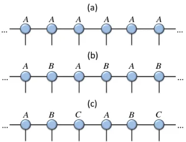
1)1dtranslational invariance and the thermodynamic limit.-In principle, all tensors in a finite-size MPS could be different, which means that the MPS itself is not translational invariant (TI). However, it is also possible to impose TI and take the thermodynamic limit of the MPS by choosing some fundamental unit cell of tensors that is repeated over the 1dlattice, infinitely-many times. This is represented in Fig.(12). For instance, if the unit cell is made of one tensor, then the MPS will be TI over one-site shifts. For unit cells of two tensors, the MPS will be TI over two-site shifts. And so on.

2) MPS are dense.-MPS can represent any quantum state of the many-body Hilbert space just by increasing sufficiently the value ofD. To coverall the states in the Hilbert space Dneeds to be exponentially large in the system size. However, it is known that low energy states of gapped local Hamiltonians in 1d can be efficiently approximated with almost arbitrary accuracy by an MPS with a finite value ofD [9]. For 1d critical systems,D tends to divergepolynomially in the size of the system [53]. These findings, in turn, explain the accuracy of some MPS-based methods for 1d systems such as DMRG. The main pictorial idea behind this property is represented in Fig.(13).

3) One-dimensional area-law.-MPS satisfy the area-law scaling of the entanglement en-tropy adapted to 1dsystems. This simply means that the entanglement entropy of a block of sites is bounded by a constant, more preciselyS(L) =−tr(ρLlogρL) =O(logD), withρL the reduced

density matrix of the block. This is exactly the behavior that is usually observed in ground states of gapped 1dlocal Hamiltonians for large sizeLof the block: precisely,S(L)∼constant forL1 [53].

(16)

Figure 12: (color online) infinite-MPS with (a) 1-site unit cell, (b) 2-site unit cell, and (3) 3-site unit cell.

Figure 13: (color online) Onion-like structure of the Hilbert space of a 1dquantum many-body system. MPS with finite bond dimension reproduce the properties of the corner of the Hilbert space satisfying the 1d area-law for the entanglement entropy. If the bond dimension increases, then the size of the manifold of accessible states also grows. For bond dimensions D sufficiently large (i.e. exponential in the sizeN of the system), MPS can actually reproduce states beyond the 1darea-law and, eventually, cover the whole Hilbert space. Compare this figure to Fig.(4).

(17)

4) MPS are finitely-correlated.-The correlation functions of an MPS decay always expo-nentially with the separation distance. This means that the correlation length of these states is always finite, and therefore MPS can not reproduce the properties of critical or scale-invariant systems, where the correlation length is known to diverge [62]. We can understand this easily with the following example: imagine that you are given a TI and infinite-size MPS defined in terms of one tensor A, as in Fig.(12.a). The two-body correlator

C(r)≡ hOiO0i+ri − hOiihO0i+ri (13)

of one-body operators Oi andOi0+rat sitesiandi+rcan be represented diagrammatically as in

Fig.(14).

Figure 14: (color online) Diagrams for the two-body correlatorC(r).

The zero-dimensional transfer matrixE_I in Fig.(15.a) plays a key role in this calculation. In particular, we have that

(E_I)r= (λ1)r D2 X µ=1 λi λ1 r ~ RTiL~i , (14)

where λi are the i= 1,2, . . . , D2 eigenvalues of EI sorted in order of decreasing magnitude, and

~

Ri, ~Litheir associated right- and left-eigenvectors. Assuming that the largest magnitude eigenvalue

λ1 is non-degenerate, forr1 we have that

(E_I)r∼(λ1)r R~1TL~1+ _λ 2 λ1 r ω+1 X µ=2 ~ RT_µ~Lµ ! , (15)

where ω is the degeneracy of λ2. Defining the matrices EO and EO0 as in Fig.(15.b), and using

the above equation, it is easy to see that

hOiOi0+ri ∼ (L~1EOR~T1)(L~1EO0R~T₁) λ2 1 + _λ 2 λ1 r−1ω+1 X µ=2 (L~1EOR~Tµ)(L~µEO0R~T₁) λ2 1 , (16)

which is expressed in terms of diagrams as in Fig.(16). In this equation, the first term is nothing but hOiihO0i+ri. Therefore,C(r) is given for larger by

C(r)∼ _λ 2 λ1 r−1ω+1 X µ=2 (L~1EOR~Tµ)(L~µEO0R~T₁) λ2 1 (17)

(18)

Figure 15: (color online) (a) Transfer matrixE_I; (b) matrixEO.

Figure 16: (color online) Diagrams for hOiO0i+ri for large separation distance r. The first part

corresponds to hOiihO0i+ri.

so that

C(r)∼f(r)ae−r/ξ (18)

with a proportionality constant a = O(ω), f(r) a site-dependent phase = ±1 if O and O0 are hermitian, and correlation lengthξ≡ −1/log|λ2/λ1|. Importantly, this type of exponential decay

of two-point correlation functions for large r is the typical one in ground states of gapped non-critical 1d systems, which is just another indication that MPS are able to approximate well this type of states.

5) Exact calculation of expectation values.-The exact calculation of the scalar product between two MPS for N sites can always be done exactly in a time O(N pD3). We explain the basic idea for this calculation in Fig.(17). For an infinite system, the calculation can be done in

O(pD3_{) using similar techniques as the ones explained above for the calculation of the two-point}

correlator C(r) (namely, finding the dominant eigenvalue and dominant left/right eigenvectors of the transfer matrix E_I). In general, expectation values of local observables such as correlation functions, energies, and local order parameters, can also be computed using the same kind of tensor manipulations.

6) Canonical form and the Schmidt decomposition.- Given a quantum state |Ψi in terms of an MPS with open boundary conditions, there is a choice of tensors calledcanonical form of the MPS [13,14] which is extremely convenient. This is defined as follows: for a given MPS with open boundary conditions (either for a finite or infinite system), we say that it is in its canonical form [14] if, for each bond index α, the index corresponds to the labeling of Schmidt vectors in

(19)

Figure 17: (color online) Order of contractions for the scalar product of a finite MPS, starting from the left. The same strategy could be used for an infinite MPS, starting with some boundary condition at infinity and iterating until convergence.

the Schmidt decomposition of|Ψiacross that index, i.e:

|Ψi= D X α=1 λα|ΦLαi ⊗ |Φ R αi. (19)

In the above equation,λαare Schmidt coefficients ordered into decreasing order (λ1≥λ2≥ · · · ≥

0), and the Schmidt vectors form orthonormal sets, that is, hΦL

α|ΦLα0i=hΦ_αR|ΦR_α0i=δαα0.

For a finite system ofN sites [13], the above condition corresponds to having the decomposition for the coefficient of the wave-function

Ci1i2...iN = Γ [1]i1 α1 λ [1] α1Γ [2]i2 α1α2λ [2] α2Γ [3]i3 α2α3λ [3] α3· · ·λ [N−1] αN−1Γ [N]iN αN−1 , (20)

where the Γ tensors correspond to changes of basis between the different Schmidt basis and the computational (spin) basis, and the vectorsλcorrespond to the Schmidt coefficients. In the case of an infinite MPS with one-site traslation invariance [14], the canonical form corresponds to having just one tensor Γ and one vectorλdescribing the whole state. Regarding the Schmidt coefficients as the entries of a diagonal matrix, the TN diagram for both the finite and infinite MPS in canonical form are shown in Fig.(18).

Figure 18: (color online) (a) 4-site MPS in canonical form; (b) infinite MPS with 1-site unit cell in canonical form.

Let us now show a way to obtain the canonical form of an MPS|Ψifor a finite system from successive Schmidt decompositions [13]. If we perform the Schmidt decomposition between the

(20)

site 1 and the remainingN−1, we can write the state as |Ψi= min(p,D) X α1=1 λ[1]α1|τ [1] α1i ⊗ |τ [2···N] α1 i, (21)

where λ[1]α1 are the Schmidt coefficients, and |τ

[1]

α1i, |τ

[2···N]

α1 i are the corresponding left and right

Schmidt vectors. If we rewrite the left Schmidt vector in terms of the local basis|i1ifor site 1, the

state|Ψican then be written as

|Ψi= p X i1=1 min(p,D) X α1=1 Γ[1]i1 α1 λ [1] α1|i1i ⊗ |τ [2···N] α1 i, (22) where Γ[1]i1

α1 correspond to the change of basis|τ

[1]

α1i= P

i1Γ

[1]i1

α1 |i1i. Next, we expand each Schmidt

vector|τα[21···N]ias |τ_α[2₁···n]i= p X i2=1 |i2i ⊗ |ω [3···N] α1i2 i. (23)

We now write the unnormalised quantum state|ω[3_α···N]

1i2 iin terms of the at mostp

2_{eigenvectors of}

the reduced density matrix for systems [3, . . . , N], that is, in terms of the right Schmidt vectors

|τα[32···n]iof the bipartition between subsystems [1,2] and the rest, together with the corresponding

Schmidt coefficientsλ[2]α2: |ω[3_α···N] 1i2 i= min(p2_,D₎ X α2=1 Γ[2]i2 α1α2λ [2] α2|τ [3···N] α2 i. (24)

Replacing the last two expressions into Eq.(22) we get

|Ψi= p X i1,i2=1 min(p,D) X α1=1 min(p2_,D₎ X α2=1 Γ[1]i1 α1 λ [1] α1Γ [2]i2 α1α2λ [2] α2 |i1i ⊗ |i2i ⊗ |τα[32···N]i. (25)

Iterating the above procedure for all subsystems, we finally get

|Ψi=X {i} X {α} Γ[1]i1 α1 λ [1] α1Γ [2]i2 α1α2λ [2] α2. . . λ [N−1] αN−1Γ [N]iN αN−1 |i1i ⊗ |i2i ⊗ · · · ⊗ |iNi, (26)

where the sum over each index in{s}and{α}runs up to their respective allowed values. And this is nothing but the representation that we mentioned in Eq.(20).

For an infinite MPS one can also compute the canonical form [14]. In this case one just needs to notice that, in the canonical form, the bond indices of the MPS always correspond to orthonormal vectors to the left and right. Thus, finding the canonical form of an MPS is commonly referred to also as orthonormalizing the indices of the MPS. For an infinite system defined by a single tensor

Athis canonical form can be found following the procedure indicated in the diagrams in Fig.(19). This can be summarized in three main steps:

(i) Find the dominant right eigenvectorV~Rand the dominant left eigenvectorV~L of the transfer

matrices defined in Fig.(19.a). Regarding the bra/ket indices,V~RandV~Lcan also be understood as

hermitian and positive matrices. Decompose these matrices as squares,VR=XX†andVL=Y†Y,

as shown in the figure.

(ii) Introduce _I = (YT₎−1_YT _and

I = XX−1 in the bond indices of the MPS as shown in

(21)

Figure 19: (color online) Canonicalization of an infinite MPS with 1-site unit cell (see text).

where U andV are unitary matrices and λ0 _{are the singular values. It is easy to show that these} singular values correspond to the Schmidt coefficients of the Schmidt decomposition of the MPS.

(iii) Arrange the remaining tensors into a new tensor Γ0, as shown in Fig.(19.c). The MPS is now defined in terms ofλ0 and Γ0.

The above procedure produces an infinite MPS such that all its bond indices correspond to orthonormal Schmidt basis, and is therefore in canonical form by construction5.

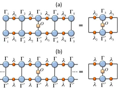
The canonical form of an MPS has a number of properties that make it very useful for MPS calculations. First, the eigenvalues of the reduced density matrices of different “left vs right” bipartitions are just the square of the Schmidt coefficients, which is very useful for calculations of e.g. entanglement spectrums and entanglement entropies. Moreover, the calculation of expectation values of local operators simplifies a lot, see the diagrams in Fig.(20).

But most importantly, the canonical form provides a prescription for the truncation of the bond indices of an MPS in numerical simulations: just keep the largestD Schmidt coefficients at every bond at each simulation step. This truncation procedure is optimal for a finite system as long as we keep the locality of the truncation (i.e. only the tensors involved in the truncated index are modified), see e.g. Ref.[13]. This prescription for truncating the bond indices turns out to be really useful, and is at the basis of the TEBD method and related algorithms for 1dsystems.

5.1.2 Some examples

Let us now give four specific examples of non-trivial states that can be represented exactly by MPS:

1) GHZ state.-The GHZ state of N spins-1/2 is given by

|GHZi=√1

2 |0i

⊗N ₊_|₁_i⊗N

, (27)

5_{Two comments are in order: first, here we do not consider the case in which the dominant eigenvalues of the} transfer matrices are degenerate. Second, this canonical form can also be achieved by running the iTEBD algorithm on an MPS with an identity time evolution until convergence [14]. Quite probably, the same result can be obtained by running iDMRG [31] with identity Hamiltonian and alternating left and right sweeps until convergence.

(22)

Figure 20: (color online) Expectation value of a 1-site observable for an MPS in canonical form: (a) 5-site MPS and (b) infinite MPS with 1-site unit cell.

where |0iand |1iare e.g. the eigenstates of the Pauli σz operator (spin “up” and “down”) [63].

This is a highly entangled quantum state of theN spins, which has some non-trivial entanglement properties (e.g. it violates certainN-partite Bell inequalities). Still, this state can be represented exactly by a MPS with bond dimension D = 2 and periodic boundary conditions. The non-zero coefficients in the tensor are shown in the diagram of Fig.(21).

Figure 21: (color online) Non-zero components for the MPS tensors of the GHZ state.

2) 1d cluster state.- Introduced by Raussendorf and Briegel [64], the cluster state in a 1d

chain can be seen as the +1 eigenstate of a set of mutually commuting stabilizer operators {K[i]_}

defined as

K[i]≡σ_zi−1σi_xσi_z+1 , (28)

where the σi_α are the usual spin-1/2 Pauli matrices with α ∈ {x, y, z} at lattice site i. Since (Ki)2=I, for an infinite system this quantum state can be written (up to an overall normalization

constant) as |Ψ1dCLi= Y i I+K[i] 2 |0i ⊗N→∞ _. ₍₂₉₎

Each one of the terms I+K[i]/2 is a projector that admits a TN representation with bond

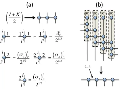
dimension 2 as in Fig.(22.a). From here, it is easy to obtain an MPS description with bond dimensionD= 4 for the 1dcluster state|Ψ1dCLi, as shown in Fig.(22.b). The non-zero coefficients

(23)

Figure 22: (color online) MPS for the 1d cluster state: (a) tensor network decomposition of the operator I+K[i]/2 and non-zero coefficients of the tensors; (b) construction of the infinite MPS

with 1-site unit cell.

Figure 23: (color online) MPS for the AKLT state: (a) spin-1/2 particles arranged in singlets

|Φi= 2−1/2(|0i ⊗ |1i − |1i ⊗ |0i), and projected by pairs into the spin-1 subspace by projectorP; (b-c) non-zero components of the tensors for the infinite MPS with 1-site unit cell: (b) in terms of _eσ1 =

√

2σ+,σe2=− √

2σ− and eσ3=σz, withσ± = (σx±σy)/2; (c) There is a gauge in which

(24)

3) 1d AKLT model.-The state we consider now is the ground state of the 1dAKLT model [65]. This is a quantum spin chain of spin-1, that is given by the Hamiltonian

H =X i ~ S[i]S~[i+1]+1 3( ~ S[i]S~[i+1])2 , (30)

where S~[i] _{is the vector of spin-1 operators at site}_i_{, and where again we assumed an infinite-size}

system. This model was introduced by Affleck, Kennedy, Lieb and Tasaki in Ref.[65], and it was the first analytical example of a quantum spin chain supporting the so-called Haldane’s conjecture: it is a local spin-1 Hamiltonian with Heisenberg-like interactions and a non-vanishing spin gap in the thermodynamic limit. What is also remarkable about this model is that its ground state is given exactly, and by construction, in terms of a MPS with bond dimension D = 2. This can be understood in terms of a collection of spin-1/2 singlets, whose spins are paired and projected into spin-1 subspaces as indicated in Fig.(23.a). This, by construction, is an MPS withD = 2. Interestingly, there is a choice of tensors for the MPS (i.e. agauge) such that these are given by the three spin-1/2 Pauli matrices, which are the generators of the irreducible representation of SU(2) with 2×2 matrices (see Fig.(23.c)). We will not enter into details of why this representation for the MPS tensors is possible. For the curious reader, let us simply mention that this is a consequence of the SU(2) symmetry of the Hamiltonian, which is inherited by the ground state, and which is also reflected at the level of the individual tensors of the MPS.

4) Majumdar-Gosh model.- We now consider the ground state of the Majumdar-Gosh model [66], which is a frustrated 1dspin chain defined by the Hamiltonian

H =X i ~ S[i]S~[i+1]+1 2 ~ S[i]S~[i+2] , (31)

whereS~[i] _{is the vector of spin-1}_/_{2 operators at site} _i_{. The ground state of this model is given by}

singlets between nearest-neighbor spins, as shown in Fig.(24). Nevertheless, to impose translational invariance we need to consider the superposition between this state and its traslation by one lattice site. The resultant state can be written in compact notation with an MPS of bond dimensionD= 3, also as shown in Fig.(24).

Figure 24: (color online) MPS for the Majumdar-Gosh state: (a) the superposition of two dimerized states of singlets|Φiin (a) can be written in terms of an infinite MPS with 1-site unit cell, with non-zero coefficients as in (b).

(25)

5.2

Projected Entangled Pair States (PEPS)

The family of PEPS [16] is just the natural generalization of MPS to higher spatial dimensions. Here we shall only consider the 2dcase. 2dPEPS are at the basis of several methods to simulate 2dquantum lattice systems, e.g. PEPS [16] and infinite-PEPS [32] algorithms, as well as Tensor Renormalization Group (TRG) [18], Second Renormalization Group (SRG) [29], Higher-Order Tensor Renormalization Group (HOTRG) [30], and methods based on Corner Transfer Matrices (CTM) and Corner Tensors [33,67, 68]. In Secs.6-7 of these notes we will describe basic aspects of some of these methods.

PEPS are TNs that correspond to a 2darray of tensors. For instance, for a 4×4 square lattice, we show the corresponding PEPS in Fig.(25), both with open and periodic boundary conditions. As such this generalization may look quite straightforward, yet we will see that the properties of PEPS are remarkably different from those of MPS. Of course, one can also define PEPS for other types of 2dlattices e.g. honeycomb, triangular, kagome... yet, in these notes we mainly consider the square lattice case. Moreover, and as expected, there are also two types of indices in a PEPS: physical indices, of dimension p, and bond indices, of dimensionD.

Figure 25: (color online) 4×4 PEPS: (a) open boundary conditions, and (b) periodic boundary conditions.

5.2.1 Some properties

We now sketch some of the basic properties of PEPS:

1) 2d Translational invariance and the thermodynamic limit.-As in the case of MPS, one is free to choose all the tensors in the PEPS to be different, which leads to a PEPS that is not TI. Yet, it is again possible to impose TI and take the thermodynamic limit by choosing a fundamental unit cell that is repeated all over the (infinite) 2d lattice, see e.g. Fig.(26). As expected for higher-dimensional systems, TI needs to be imposed in all the spatial directions of the lattice.

2) PEPS are dense.-As was the case of MPS, PEPS is a dense family of states, meaning that they can represent any quantum state of the many-body Hilbert space just by increasing the value of the bond dimension D. As happens for MPS, the bond dimension D of a PEPS needs to be exponentially large in the size of the system in order to cover the whole Hilbert space. Nevertheless, one expectsD to be reasonably small and finite for low-energy states of interesting 2dquantum models. In practice this is observed numerically [32], but there are also theoretical arguments in favor of this property. For instance, it is well known that D = 2 is sufficient to

(26)

Figure 26: (color online) Infinite PEPS with (a) 1×1 unit cell, (b) 2×2 unit cell with 2 tensors, (c) 2×2 unit cell with 4 tensors, and (d) 2×3 unit cell with 6 tensors.

handle polynomially-decaying correlation functions (and hence critical states) [69], and that PEPS can also approximate with arbitrary accuracy thermal states of 2dlocal Hamiltonians [57]. In this case, a similar picture to the one in Fig.(13) would also apply adapted to the case of PEPS and the 2darea-law.

3)2dArea-law.-PEPS satisfy also the area-law scaling of the entanglement entropy. This was shown already in the example of Fig.(10), but the validity is general. In practice, the entanglement entropy of a block of boundaryLof a PEPS with bond dimensionD is alwaysS(L) =O(LlogD). As discussed before, this property is satisfied by many interesting quantum states of quantum many-body systems, such as some ground states and low-energy excited states of local Hamiltonians.

4) PEPS can handle polynomially-decaying correlations.-A remarkable difference be-tween PEPS and MPS is that PEPS can handle two-point correlation functions that decay poly-nomially with the separation distance [69]. And this happens already for the smallest non-trivial bond dimension D = 2. This property is important, since correlation functions that decay poly-nomially (as opposed to exponentially) are characteristic of critical points, where the correlation length is infinite and the system is scale invariant. Hence, the class of PEPS is suitable to describe, in principle, gapped phases as well as critical states of matter.

This property can be seen with the following example [69]: consider the unnormalized state

(27)

with|+i= 2−1/2(|0i+|1i), andH given by

H=− X

h~r,~r0_i

σ_z[~r]σ[_z~r0] . (33)

After some simple algebra it is easy to see that the norm of this quantum state is proportional to the partition function of the 2dclassical Ising model on a square lattice at inverse temperatureβ, i.e.:

hΨ(β)|Ψ(β)i ∝Z(β) =X {s}

e−βK({s}), (34)

withK({s}) the classical Ising Hamiltonian,

K({s}) =− X

h~r,~r0_i

s[~r]s[~r0] , (35)

where s[~r] ₌ _±_{1 is a classical spin variable at lattice site} _~_r_{, and} _{_s_} _{is some configuration of}

all the classical spins. It is also easy to see that the expectation values of local operators in

|Ψ(β)icorrespond to classical expectation values of local observables in the classical model. For instance, the expectation value ofσz[~r]corresponds to the classical magnetization at site~rat inverse

temperatureβ, hs[~r]iβ= hΨ(β)|σz[~r]|Ψ(β)i hΨ(β)|Ψ(β)i = 1 Z(β) X {s} s[~r]e−βK({s}) . (36)

Also, the two-point correlation functions in the quantum state correspond to classical correlation functions of the classical model. For instance, the correlation function for operators σz[~r] and σ

[~r0_] z

at sites~rand~r0 corresponds to the usual correlation function of the classical Ising variables,

hs[~r]s[~r0]iβ = hΨ(β)|σz[~r]σ [~r0_] z |Ψ(β)i hΨ(β)|Ψ(β)i = 1 Z(β) X {s} s[~r]s[~r0]e−βK({s}). (37)

At the critical inverse temperatureβc = (log(1+

√

2))/2 it is well known that the correlation length of the system diverges, and the above correlation function decays polynomially for long separation distances as

hs[~r]s[~r0]iβc ≈

a

|~r−~r0_|1/4 , (38)

for some constant a = O(1) and |~r−~r0| 1. The next step is to realize that, actually, the quantum state |Ψ(β)i is a 2d PEPS with bond dimension D = 2. This is shown in the tensor network diagrams in Fig.(27). Therefore, at the critical valueβ =βc, the resultant quantum state

|Ψ(βc)i is an example of a 2d PEPS with finite bond dimension D = 2 and with polynomially

decaying correlation functions (and hence infinite correlation length).This should be considered as a proof of principle about the possibility of having some criticality in a PEPS with finite bond dimension. As a remark, notice that this is totally different to the case of 1dMPS, where we saw before that two-point correlation functions always decay exponentially fast with the separation distance.

Notice, though, that the criticality obtained in this PEPS is essentially classical, since we just codified the partition function of the 2dclassical Ising model as the squared norm of a 2dPEPS. Recalling the quantum-classical correspondence that a quantum d-dimensional lattice model is equivalent to some classicald+ 1-dimensional lattice model [70], one realizes that this criticality is actually the one from the 1dquantum Ising model, but “hidden” into a 2dPEPS with smallD. By generalizing this idea, we could actually think as well of e.g. “codifying” the quantum criticality of a 2dquantum model into a 3dPEPS with smallD. Yet, it is still unclear under which conditions a 2dPEPS could handle this true 2dquantum criticality for smallD as well.

(28)

Figure 27: (color online) PEPS for a (classical) thermal state: (a) tensor network decomposition of the operator exp(−βσz[~r]σ[~r

0_]

z /2) and non-zero coefficients of the tensors; (b) construction of the

infinite PEPS with 1-site unit cell.

5) Exact contraction is ]P-Hard: The exact calculation of the scalar product between two PEPS is an exponentially hard problem. This means that for two arbitrary PEPS of N

sites, it will always take a time O(exp(N)), no matter the order in which we try to contract the different tensors. This statement can be done mathematically precise. From the point of view of computational complexity, the calculation of the scalar product of two PEPS is a problem in the complexity class ]P-Hard [71]. We shall not enter into detailed definitions of complexity classes here, yet let us explain in plain terms what this means. The class ]P-Hard is the class of problems related to counting the number of solutions to NP-Complete problems. Also, the class NP-Complete is commonly understood as a class of very difficult problems in computational complexity6_{, and it is widely believed that there is no classical (and possibly quantum) algorithm}

that can solve the problems in this class using polynomial resources in the size of the input. A similar statement is also true for the class]P-Hard. Therefore, unlike for 1dMPS, computing exact scalar products of arbitrary 2dPEPS is, in principle, inefficient.

However, and as we will see in Sec.6, it is possible in practice to approximate these expectation values using clever numerical methods. Moreover, recent promising results in the study of entan-glement spectra seem to indicate that these approximate calculations can be done with a very large accuracy (possibly even exponential), at least for 2d PEPS corresponding to ground states of gapped, local 2dHamiltonians [73].

6) No exact canonical form.- Unlike for MPS with open boundary conditions, there is no canonical form of a PEPS, in the sense that it is not possible to choose orthonornal basis simultaneously for all the bond indices. In fact, this happens already for MPS with periodic boundary conditions or, more generally,as long as we have a loop in the TN. Loosely speaking, a loop in the TN means that we can not formally split the network into left and right pieces by just cutting one index, so that a Schmidt decomposition between left and right does not make sense. In practice this means that we can not define orthonormal basis (i.e. Schmidt basis) to the left and

(29)

right of a given index, and hence we can not define a canonical form in this sense (see Fig.(28)).

Figure 28: (color online) By “cutting” a link in a TN, one can define left and right pieces if there are no other connecting indices between the two pieces (a), whereas this is not possible if other connecting indices exist (b).

Nevertheless, it is observed numerically that for non-critical PEPS it is usually possible to find a quasi-canonical form, which leads to approximate numerical methods for finding ground states (a variation of the so-called “simple update” approach [74]). We refer the interested reader to Ref.[75] for more details about this.

5.2.2 Some examples

In what follows we provide some examples of interesting quantum states for 2dlattices that can be expressed exactly using the PEPS formalism. These are the following:

1) 2d Cluster State.-The cluster state in a 2d square lattice [64] is highly-entangled quan-tum state that can be used as a resource for performing universal measurement-based quanquan-tum computation. This quantum state is the +1 eigenstate of a set of mutually commuting stabilizer operators{K[~r]}defined as

K[~r]≡σ_x[~r] O

~ p∈Γ(~r)

σ_z[p~] , (39)

where Γ(~r) denotes the four nearest-neighbor spins of lattice site ~r and the σ[α~r] are the usual

spin-1/2 Pauli matrices with α∈ {x, y, z} at lattice site ~r. For the infinite square lattice, these stabilizers are five-body operators. Noticing that (K[~r]₎2₌

I, this quantum state can be written

(up to an overall normalization constant) as

|Ψ2dCLi= Y ~ r I+K[~r] 2 |0i ⊗N→∞ _. ₍₄₀₎

Each one of the terms I+K[~r]/2 is a projector that admits a TN representation as in Fig.(29).

From here, it is easy to obtain a TN description for the 2dcluster state|Ψ2dCLiin terms of a 2d

PEPS with bond dimension D = 4, as shown in Fig.(29). In the figure we also give the value of the non-zero coefficients of the PEPS tensors.

2) Toric Code model.-The Toric Code, introduced by Kitaev [76], is a model of spins-1/2 on the links of a 2dsquare lattice. The Hamiltonian can be written as

H =−Ja X s As−Jb X p Bp , (41)

(30)

Figure 29: (color online) PEPS for the 2dcluster state: (a) tensor network decomposition of the operator I+K[~r]/2 and non-zero coefficients of the tensors; (b) construction of the infinite PEPS

with 1-site unit cell.

whereAsandBp are star and plaquette operators such that

As= Y ~r∈s σ_x[~r] , Bp= Y ~ r∈p σ_z[~r] . (42)

In other words,Asis the product ofσxoperators for the spins around a star, andBpis the product

ofσzoperators for the spins around a plaquette. Here we will be considering the case of an infinite

2dsquare lattice.

The Toric Code is of relevance for a variety of reasons. First, it can be seen as the Hamiltonian of a _Z2 lattice gauge theory with a “soft” gauge constraint [77] (i.e. if we send either Ja or Jb

to infinity, then we recover the low-energy sector of the lattice gauge theory). But also, it is important because it is the simplest known model such that its ground state displays the so-called “topological order”, which is a kind of order in many-body wave-functions related to a pattern of long-range entanglement that prevades over the whole quantum state (here we shall not discuss topological order in detail; the interested reader can have a look at the vast literature on this topic, e.g. Ref.[4]). Furthermore, the Toric Code is important in the field of quantum computation, since one could use its degenerate ground state subspace on a torus geometry to define a topologically protected qubit that is inherently robust to local noise [76].

An interesting feature about the Toric Code is that, again, it can be understood as a sum of mutually commuting stabilizer operators. This time the stabilizers are the set of star and plaquette operators{As}and{Bp}. As for the cluster state, it is easy to check that the square of

the stabilizer operators equals the identity (A2

s=Bp2 =I ∀s, p). The ground state of the system

is the +1 eigenstate of all these stabilizer operators. For an infinite 2dsquare lattice this ground state is unique, and can be written (up to a normalization constant) as

|ΨT Ci= Y s (I+As) 2 Y p (I+Bp) 2 |0i ⊗N→∞₌Y s (I+As) 2 |0i ⊗N→∞ _, ₍₄₃₎

where the last equality follows from the fact that the state |0i⊗N→∞ _{is already a +1 eigenstate} of the operators Bp for any plaquettep. The above state can be written easily as a PEPS with

bond dimensionD = 2 [69]. For this, notice that each one of the terms (_I+As)/2 for any star s

admits the TN representation from Fig.(30.a). From here, a PEPS representation with a 2-site unit cell as in Fig.(26.b) follows easily, see Fig.(30.b). As we can see with this example, a PEPS with

(31)

Figure 30: (color online) PEPS for the Toric Code: (a) tensor network decomposition of operator (_I+As)/2 and non-zero coefficients of the tensors; (b) construction of the infinite PEPS with 2×2

unit cell and 2 tensors.

the smallest non-trivial bond dimensionD= 2 can already handle topologically ordered states of matter.

3) 2d Resonating Valence Bond State.- The 2d Resonating Valence Bond (RVB) state [78], is a quantum state proposed by Anderson in 1987 in the context of trying to explain the mechanisms behind high-Tc superconductivity. For our purposes this state corresponds to the

equal superposition of all possible nearest-neighbor dimer coverings of a lattice, where each dimer is a SU(2) singlet,

|Φi=√1

2(|0i ⊗ |1i − |1i ⊗ |0i) , (44)

which is a maximally-entangled state of two qubits (also known as EPR pair, or Bell state). For the 2dsquare lattice this is represented in Fig.(31.a). This state is also important since it is the arquetypical example of a quantum spin liquid: a quantum state of matter that does not break any symmetry (neither translational symmetry, nor SU(2)). Importantly, this RVB state can also be written as a PEPS with bond dimension D = 3. The non-zero coefficients of the tensors are given in Fig.(31.b).

Figure 31: (color online) A 2dResonating Valence Bond state built from nearest-neighbor singlets (a) can be written as an infinite PEPS with 1-site unit cell, with non-zero coefficients of the tensors as in (b).

(32)

4) 2d AKLT model.-The 2d AKLT model on a honeycomb lattice [65, 79] is given by the Hamiltonian H = X h~r,~r0_i ~ S[~r]S~[~r0]+116 243 ~ S[~r]S~[~r0] 2 + 16 243 ~ S[~r]S~[~r0] 3 , (45)

whereS~[~r] _{is the vector of spin-3}_/_{2 operators at site}_~_r_{, and the sum is over nearest-neighbor spins.}

As explained in Ref.[65, 79], this model can be seen as a generalization of the 1d AKLT model in Eq.(30) to two dimensions. The ground state can be understood in terms of a set of spin-1/2 singlets, which are brought together into groups of 3 at every vertex of the honeycomb lattice, and projected into their symmetric subspace (i.e. spin-3/2), see Fig.(32). By construction, this is a 2d

PEPS with bond dimension D= 2.

Figure 32: (color online) PEPS for the 2dAKLT state on the honeycomb lattice. Spin-1/2 particles arranged in singlets |Φi = 2−1/2₍_|₀_{i ⊗ |}₁_{i − |}₁_{i ⊗ |}₀_i_{), and projected in trios using projector}

P = (|1ih0| ⊗ h0| ⊗ h0|+|2ih1| ⊗ h1| ⊗ h1|+|3ihW|+|4ihW¯|), with |Wi= 3−1/2₍_|₀_{i ⊗ |}₀_{i ⊗ |}₁_i₊

|0i ⊗ |1i ⊗ |0i+|1i ⊗ |0i ⊗ |0i) and|W¯i= 3−1/2₍_|₁_{i ⊗ |}₁_{i ⊗ |}₀_i₊_|₁_{i ⊗ |}₀_{i ⊗ |}₁_i₊_|₀_{i ⊗ |}₁_{i ⊗ |}₁_i_).

6

Extracting information: computing expectation values

An important problem for TN is how to extract information from them. This is usually achieved by computing expectation values of local observables. It turns out that such expectation values can be computed efficiently, either exactly (for MPS) or approximately (for PEPS). This is very important, since otherwise it would not make any sense to have an efficient representation of a quantum state: we also need to be able to extract information from it!

In what follows we explain how expectation values can be extracted efficiently from MPS and PEPS, both for finite and infinite systems. In fact, in the case of MPS with open boundary conditions a lot of the essential information was already introduced in Sec.4, when talking about the exponential decay of two-point correlation functions and the exact calculation of norms.

We will see that the calculation of expectation values follows many times adimensional reduc-tion strategy. More precisely, the 1d problem for an MPS is reducible to a 0dproblem, and this can be solved exactly. Also, the 2dproblem for a PEPS is reducible to a 1dproblem that can be solved approximately using MPS techniques. This MPS problem, in turn, is itself reducible to a 0dproblem that is again exactly solvable. Such a dimensional reduction strategy is nothing but an implementation, in terms of TN calculations, of the ideas of the holographic principle [1].

6.1

Expectation values from MPS

Expectation values of local operators can be computed exactly for an MPS without the need for further approximations. In the case of open boundary conditions, this is achieved for finite and

(33)

infinit