Unsupervised learning for image classification

(1)

Instructor

Unsupervised Learning for Image Classication

Yao Lu

Helsinki December 8, 2015 UNIVERSITY OF HELSINKI Department of Computer Science

(2)

Faculty of Science Department of Computer Science Yao Lu

Unsupervised Learning for Image Classication Computer Science

December 8, 2015 52 pages + 0 appendices

Unsupervised Learning, Convolutional Neural Networks, Deep Learning, Image Classication This thesis is an investigation of unsupervised learning for image classication. The state-of-the-art image classication method is Convolutional Neural Network (CNN), which is a purely supervised learning method. We argue that despite of the triumph of supervised learning, unsupervised learning is still important and compatible with supervised learning. For example, in the situation where some classes have no training data at all, so called zero-shot learning task, unsupervised learning can leverage supervised learning to classify the images of unseen classes. We proposed a new zero-shot learning method based on CNN and several unsupervised learning algorithms. Our method achieves the state-of-the-art results on the largest public available labelled image dataset, ImageNet fall2011.

ACM Computing Classication System (CCS): A.1 [Introductory and Survey],

I.7.m [Document and text processing]

Tekijä Författare Author

Työn nimi Arbetets titel Title

Oppiaine Läroämne Subject

Työn laji Arbetets art Level Aika Datum Month and year Sivumäärä Sidoantal Number of pages

Tiivistelmä Referat Abstract

Avainsanat Nyckelord Keywords

Säilytyspaikka Förvaringsställe Where deposited

(3)

1 Introduction

Biological vision systems are remarkably powerful. We can recognize an old friend among a hundred of strangers, despite of the changes of pose, clothing, background and viewpoint. How is this possible? How does vision work?

Figure 1: Descartes' the-ory of vision.2

Philosophers and scientists have been investigating and speculating on vision since hundreds of years ago. In his book Principles of Philosophy published in 1644, Descartes developed his over-simplied mechanistic the-ory of vision as illustrated in Figure 1. In 1966, re-searchers in MIT tried to solve vision in a summer and only found vision is much more dicult than what they once thought [Pap66]. Even to date, we still do not have a full understanding of biological vision.

Our knowledge of vision would enable us to build arti-cial vision systems [Fuk88, LBBH98]. Such vision sys-tems can be employed for autonomous driving, image

search, biometric recognition, surveillance and robots. On the other hand, in the process of building articial vision systems, we could discover principles of vision, which in turn help us understand biological vision systems [CHY+_{14]. Building}

ar-ticial vision systems has a long history of over 50 years [AT13], from early systems based on volumetric parts to modern ones based on articial neural networks. The primary goal of a vision system, either biological or articial, is visual recogni-tion, the ability to perceive an scene or object's physical properties such as shape, color and texture. According to [Per09], there are ve visual recognition tasks, in order of diculty:

• Verication. Test if an area of an image contains a particular object.

• Detection and localization. Finding where is a particular object in an image. • Classication. Classifying an image into a number of categories.

• Naming. Name and locate all objects in an image. • Description. Given an image, describe it by text. 2_{Image from Principles of Philosophy 1664.}

(5)

In this thesis, we focus on the (image) classication task, which has been and still is an active research area in computer vision.

1.1 Problem Statement

The current state-of-the-art image classication method is Convolutional Neural Network (CNN) [LBBH98]. It has been employed as the workhorse for a number of image classication competitions [CMS12, KSH12, SLJ+_{15]. Moreover, CNN}

has already been employed widely in the industry, for example, Google and Baidu's content-based image retrieval system. It has been shown that CNN can even surpass humans in recognizing 1000 objects [SLJ+_15].

However, there is a severe problem with CNN: it requires a large amount of labelled data. The acquisition of labelled data is very time-consuming and expensive. It requires human annotators to manually observe each data point and input the correct labels. For more specialized domain such as medical and satellite imaging, it requires experts to annotate the images. The number of qualied domain experts are rather limited, making the labelling even more expensive. And since the possible values that data can take are exponentially many, it is impractical to obtain a suciently large amount of labelled data.

In order to reduce the dependence of CNN on labelled data, we have to explore the realm of unlabelled data. Compared to labelled data, unlabelled data is numer-ous and can be obtained cheaply. Learning from unlabelled data is unsupervised learning. The pursuit of unsupervised learning for image classication started in 2006 [HOT06]. Despite of intensive research on this topic, current state-of-the-art image classication method, CNN, is a purely supervised learning method. Unsu-pervised learning methods such as sparse coding and pre-training are unnecessary for obtaining high-performance image classication [CMS12, KSH12, SLJ+_15].

Is unsupervised learning a dead end for image classication? In a recent Nature paper [LBH15], neural network researchers LeCun, Bengio and Hinton pointed out this embarrassing situation. However, they still hold optimistic attitude towards unsupervised learning.

Unsupervised learning had a catalytic eect in reviving interest in deep learning, but has since been overshadowed by the successes of purely su-pervised learning...We expect unsusu-pervised learning to become far more

(6)

important in the longer term. Human and animal learning is largely un-supervised: we discover the structure of the world by observing it, not by being told the name of every object. - LeCun, Bengio and Hinton

The integration of unsupervised learning for image classication remains elusive. Therefore, the central question in this thesis is:

While the state-of-the-art image classication methods are purely supervised, can unsupervised learning algorithms still be use-ful?

1.2 Contributions

We showcase that unsupervised learning is useful in the context of zero-shot learn-ing. Zero-shot learning is a (image) classication task in which some classes have no training data at all. The main contribution of this thesis is: based on the several unsupervised learning algorithms, we proposed a new zero-shot learning method, which is compatible to supervised learning. The eectiveness of our pro-posed method is demonstrated on the largest public available labelled image dataset, ImageNet 2011fall, which has over 14.2 million images and over 20000 object classes. In Section 2, we review all the background knowledge which is necessary for under-standing our zero-shot learning method. In Section 3, we formally introduce our zero-shot learning method. In Section 4, we conclude this thesis and discuss its implications and future research directions.

2 Background Knowledge

2.1 Image Classication

Image classication is a fundamental problem in computer vision. It is the task of classifying images into a number of categories. Image classication is the basis for higher level tasks such as object detection and image description, as explained in Section 1. It has been an active research area in computer vision over 50 years [AT13]. Despite of the eorts of 50 years, we still do not have a computer vision system which can achieve human level recognition ability for images in the wild. Image classication is dicult due to the variations inherent to images such as

(7)

translation, scaling, rotation and luminance changes. We divide image classication methods into two families: traditional methods and Convolutional Neural Networks. 2.1.1 Traditional Methods

The traditional image classication methods typically have four stages: feature ex-traction, quantization, pooling, and classier.

Feature Extraction Quantization Pooling Classier

Images _Prediction

Figure 2: Traditional image classication pipeline.

Feature Extraction Feature extraction is the rst stage of the traditional im-age classication pipeline. Its job is to extract low-level discriminative local visual features such as edge and corner, which will be used for the next stage. Feature extraction is typically done in a convolutional or sliding window manner across the whole image (dense sampling). Dierent features are dened by dierent convolution kernels. See Figure 3 for an illustration of convolution.

Figure 3: Convolution.3

A classical type of features is Gabor. A Gabor feature can be understood as a Gaussian envelope of a two-dimensional sinusoidal function,

g(x, y, λ, θ, ψ, σ, γ) = exp(−x 02₊_γ2_y02 2σ2 ) cos(2π x0 λ +ψ) (1) x0 =xsinθ+ycosθ, (2) y0 =−xcosθ+ysinθ, (3)

(8)

wherexandyare image position,λ is the wavelength parameter of the sinusoidal,θ

is the orientation parameter, ψ is the phase parameter,σ is the standard deviation

parameter of the Gaussian envelope and γ is the ellipticity parameter of the Gabor

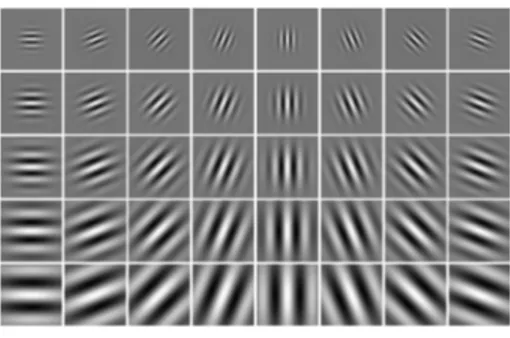
function. From Figure 4, we can see Gabor features are sensitive to direction and frequency.

Figure 4: Gabor features.4

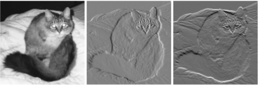
Another well-known type of features is scale-invariant feature transform (SIFT) [Low99]. SIFT features have robustness to scale, rotation and illumination changes. They based on histograms of image gradients. Image gradient is a directional change in the intensity or color in an image. It is used for extracting information such as edges. To obtain the image gradient along horizontal (x-axis) and vertical directions

(y-axis), apply the following lters to an image, respectively.

Gx = [−1 0 1] Gy = [−1 0 1]T (4)

The results of the ltering can be seen in Figure 5. The gradient magnitude is G=qG2

x+G2y (5)

and the gradient orientation or direction is

Θ=atan2(Gy,Gx) (6)

The feature extraction process of SIFT works as follows: For an image position, a 16x16 neighbourhood is taken. It is divided into 16 sub-blocks of size 4x4. For each sub-block, 8 bin histogram of image gradient orientations is created. As a result, a total of 128-dimensional feature vector is created. See Figure 6 for illustration. A more recent approach is unsupervised feature learning including sparse coding [OF97] and Independent Component Analysis (ICA) [HKO04]. For example, the

4_Image _from _{http://www.mathworks.com/matlabcentral/fileexchange/}

(9)

Figure 5: Image gradient. Left: original image. Middle: ltered image by applying Gx. Right: ltered image by applying Gy.6

Figure 6: SIFT feature.7

features learned by ICA on natural image patches resemble the Gabor features due to their orientation, scaling and frequency selectivity. The details of these algorithms will be discussed in the Section 2.2. For a comprehensive review of unsupervised feature learning, see [BCV13].

Quantization Quantization or codebook learning is to build high-level features by aggregating low-level features in the previous stage. Since the amount of low-level of features are typically enormous, a quantization method is needed so as to keep the number of features manageable.

The simplest way of doing quantization is usingk-means clustering. Each low-level

feature is then assigned to its nearest cluster centroid. Then the assignments of low-level features instead of their real valued vectors are passed to the next stage. A more sophisticated codebook learning method is Fisher vectors [PD07, PSM10].

6_{Image from https://en.wikipedia.org/wiki/Image_gradient.} 7_{Image from http://www.aishack.in/.}

(10)

Fisher vectors are based on Gaussian mixture model, which is a generalization of

k-means clustering. Therefore, Fisher vectors can be seen as an extension of the k-means clustering quantization.

Pooling Pooling is to aggregate the local features for whole image representation by a single vector. The simplest way of pooling is bag-of-features [FFP05], which uses the histogram of the high-level features as the vector representation of an image, as in Figure 7. However, bag-of-features pooling ignores the spatial relationship layout of the local features, which would cause ambiguity and loss in classication accuracy. An improved pooling method is spatial pyramid matching [LSP06], which uses bag-of-features at multi-scale grids of the image. The feature vectors created at multi-scale are then concatenated as a single vector. See Figure 8 for illustration.

Figure 7: Bag of features.8

Figure 8: Spatial pyramid matching.9

8_{Image from http://cs.brown.edu/courses/cs143/2011/results/proj3/senewman/.} 9_{Image from [LSP06].}

(11)

Classier The most popular classier in the traditional image classication pipeline is support vector machine (SVM) [CV95], which is a linear classier such that the decision function is

g(x) = sign(f(x)) where

f(x) =w·x+b

The objective function of SVM (primal form) has the following min w 1 2kwk+C X i l(xi, yi) (7)

where C is a hyper-parameter and l(·) is so-called hinge-loss and takes the form of

l(x, y) = max(0,1−yf(x))) (8) Sincel(·)is not dierentiable, sub-gradient methods such as Pegasos [SSSSC11] are used for ecient optimization.

Kernel SVM is often used when the amount of data is not large. Kernel method makes SVM a nonlinear classier, which could lead to higher classication accuracy. Typically used kernels include

• Histogram intersection kernel

K(x,x0) = N X i=1 min(xi, x0i) (9) • Gaussian kernel K(x,x0) = exp(−kx−x 0_k2 σ2 ) (10) • χ2 (Chi-square) kernel K(x,x0) = N X i=1 (xi−x0i)2 xi+x0i (11)

It is dicult to decide beforehand which kernel to use in practice. The performance of each kernel depend on the data at hand. It is suggested to try all of them based

(12)

on validation error. Kernel SVM has the following objective function (dual form) min α 1 2 X i,j αiαjK(xi,xj)− X i yiαi (12) s.t.X i αi = 1,0≤yiαi ≤C (13)

The decision function of kernel SVM is

g(x) =sign(X

i

αiK(xi,x) +b) (14)

When we have a large amount of high dimensional data, linear SVM would suce for achieving high classication accuracy. For multi-class classication, one-vesus-rest strategy is typically used.

Summary In machine learning, it is a rule-of-thumb that features matter more than classiers to classication accuracy [Dom12]. Good features need to be tolerant to transformations such as translation, orientation and viewpoint changes. On the other hand, good features also need to be discriminative so that they can distinguish dierent objects. One lesson that traditional image classication methods have taught us is the importance of local features. Global features of an image could change substantially even for slight transformations. For example, consider a global feature (lter) whose size is as large as the image. Even for only slight translations of the image, the output of the lter would change signicantly. On the other hand, the response of a local feature would stay the same. Only the position of the response changes. Another lesson is: one can aggregate local features to form invariant high-level abstract features, which is critical to classication accuracy. Traditional image classication methods were employed for winning several large scale image classication competitions such as ImageNet ILSVRC 2010 [LLZ+11]

and ImageNet ILSVRC 2011 [SP11] competitions. they were the state-of-the-art image classication methods until CNN came into stage [KSH12].

2.1.2 Convolutional Neural Network (CNN)

CNN shares a similar image classication pipeline as the traditional methods. How-ever, while in the traditional image classication pipeline only the classier is trained with labelled data, CNN is trained end-to-end, which means all the stages (feature

(13)

extraction, quantization, pooling and classier) are learnable. CNN is the cur-rent state-of-the-art image classication method in various datasets such as MNIST [LBBH98], CIFAR-10 [KH09] and ImageNet [DDS+_09].

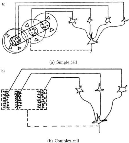
The architecture of Convolutional Neural Network (CNN) rooted from the seminal work of the discovery of simple cells and complex cells in the brain by neuroscientists Hubel and Wiesel. Simple cells receive inputs from the receptive elds of LGN neurons. And complex cells the sum or pool the outputs from simple cells. See Figure 9 for illustration.

(a) Simple cell

(b) Complex cell

Figure 9: Hubel and Wiesel's cells.10

Inspired by Hubel and Wiesel, Fukushima proposed Neocognitron [Fuk88]. Neocog-nitron is a neural network model which uses articial simple-cell layers and complex-cell layers alternatively, so as to achieve small translation invariance. However, Fukushima only proposed the Neocognitron architecture, without a learning algo-rithm. Therefore, Neocognitron is not a practical image classication method.

(14)

Figure 10: Neocognitron.11

LeCun [LBBH98] proposed CNN, which has a more simplied architecture as Neocog-nitron and a learning algorithm. LeCun applied the back-propagation algorithm [Wer82, RHW88] to learn all the weights of CNN and achieved the state-of-the-art results on MNIST. Moreover, he invented various tricks for speeding up the training and reduce the generalization error of CNN [LBOM12].

Figure 11: Convolutional Neural Network.12

Architecture In the following we list the key components of CNN architecture, including the classic ones and more recently ones

• Convolution layer. Convolution corresponds to the local feature extraction in

the traditional image classication pipeline. The denition of two-dimensional

11_{Image from [Fuk88].}

(15)

convolution is y[i, j] = M X m=0 N X n=0 x[m, n]k[i−m, j −n] (15)

where, for image position(x, y), x[i, j]is the pixel value of the original image,

k[i, j] is the pixel value of the convolution kernel, y[i, j] is the pixel value of the ltered image,M is the height of the original image andN is the width of

the original image. Convolution is a heavy operation due to the size of images and the number of convolution kernels in CNN. Therefore, ecient convolution techniques are needed. There are two much techniques which are commonly used:

1. Conversion to matrix multiplication. Convolution can be formulated into matrix multiplication. Since there are many highly optimized matrix multiplication libraries such as OpenBLAS13 _{for CPU and CuBLAS}14 _for

GPU, convolution can be done with higher speed than a naive implemen-tation. To see how the conversion is possible, we give an example. For two matrices to convolute, the following equation holds

   a11 a12 a13 a21 a22 a23 a31 a32 a33   ⊗ b11 b12 b21 b22 ! =       a11 a12 a21 a22 a12 a13 a22 a23 a21 a22 a31 a32 a22 a23 a32 a33             b11 b12 b21 b22      

where ⊗ is the convolution operator.

2. Fast Fourier Transform (FFT). The convolution theorem allow us to con-vert a convolution operation into a multiplication operation with Fourier transform. For a matrix of of elements n, a naive Fourier transform

al-gorithm has time complexity O(n2₎ _{but FFT only has time complexity}

O(nlogn). For two matrices of elementsm andn, the time complexity of

naive convolution is O(mn). And the time complexity of the FFT-based convolution is O(mlogm+nlogn). If m and n are both large, we have

a performance gain using the FFT-based convolution. However, in CNN, usually the convolution kernel are rather small. For example, 7×7, 5×5,

3×3 and even 1×1. However, if there are a large number convolution

kernels, performance gain can be achieved, as shown in [MHL13].

13_{http://www.openblas.net/}

(16)

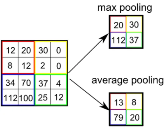
• Pooling layer. Pooling in CNN corresponds to the pooling in the traditional

image classication pipeline. See Figure 12 for illustration.

Figure 12: Max pooling and average pooling.15

There two commonly used pooling methods: average pooling and max pooling, as illustrated in Figure 12. Average pooling was proposed in original Le-Net architecture of CNN [LBBH98]. Max pooling was rst used in the HMAX model [RP99], which is also a deep neural network with convolution. However, HMAX is not trained end-to-end as CNN. In [CMS12], CNN with max pooling was rst used to win several visual recognition competitions [CMS12]. A theoretical analysis of the two pooling methods can be found in [BPL10].

• Fully connected layer. Fully connected layer is the same as the hidden layer

in Multi-layer Perceptrons [RHW88]. It acts as a nonlinear transformation for the output classier.

• Softmax layer. The softmax layer is the classier of CNN. It takes inputs

y= (y1, ..., yn) and outputs vector x= (x1, ..., xn) such that

xi =

exp(yi/T)

P

jexp(yj/T)

(16) whereT is the temperature parameter.

• Network in network layer. The convolution layer provides linear convolution.

In order to achieve nonlinear convolution, we can replace the convolutional kernel, a matrix, with a Multi-layer Perceptron. This results in network in network [MLY14] layer, as illustrated in Figure 13.

(17)

Figure 13: Network in network layer.16

• Inception. The inception layer is essentially a multi-resolution convolution

layer. As illustrated in Figure 14, It concatenates 1×1, 3×3, and 5×5

convo-lution operations. It was rst employed in GoogLeNet [SLJ+_{15] for winning}

the ImageNet ILSVRC 2014 competition.

Figure 14: Inception layer.17

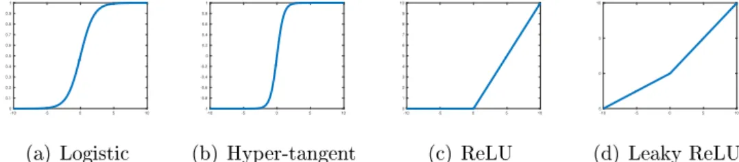
• Activation functions. There are several activation functions commonly used:

1. Logisitic

f(x) = 1

1 + exp(−x) 2. Hyper-tangent

f(x) = tanh(x)

16_{Image from [MLY14].} 17_{Image from [SLJ}+_15].

(18)

-10 -5 0 5 10 0 0.1 0.2 0.3 0.4 0.5 0.6 0.7 0.8 0.9 (a) Logistic -10 -5 0 5 10 -1 -0.8 -0.6 -0.4 -0.2 0 0.2 0.4 0.6 0.8 (b) Hyper-tangent -10 -5 0 5 10 0 1 2 3 4 5 6 7 8 9 (c) ReLU -10 -5 0 5 10 -5 0 5 (d) Leaky ReLU

Figure 15: Activation functions. 3. Rectier linear unit (ReLU)

f(x) = max(0, x) 4. Leaky rectier linear unit (Leaky ReLU)

f(x) =    x, x≥0 x a, <0

where a is a parameter to be learned or xed.

(a) ReLU (solid line) vs. Hyper-tangent (dashed line)

(b) ReLu vs. Leaky ReLU

Figure 16: Convergence of training a CNN on CIFAR-10 with dierent activation functions.19

It has been shown that ReLU gives much faster convergence than sigmoid functions such as logistic and hyper-tangent in training a CNN [KSH12], as in Figure 16 (a). And in [XWCL15], it has been shown that Leaky ReLU outperforms ReLU, as shown in Figure 16 (b).

(19)

Training The training of CNN typically takes a large amount of time and compu-tational resources compared to traditional methods. The success of training CNN depends highly on the hyper-parameters, which take great eorts to tune. Here we list several techniques which are commonly used.

• propagation [RHW88]. This is the workhorse for training CNN.

Back-propagation is a recursive method for calculating the gradient of the the cost function of a CNN.

• Stochastic gradient descent [RM51]. Instead of using all training data (batch)

for each iteration, stochastic gradient descent typically uses a mini-batch for each iteration of updating the parameters. It has sound theoretical foundations and works well in practice. It generally takes the following form

θ(t+1) =θ(t)−η(t)∇θL(θ(t)) (17)

whereθ is the parameter, η is the learning rate andL is the cost function. • Momentum [RHW88]. Stochastic gradient descent usually has high variance

and therefore slow convergence speed. In order to stabilize stochastic gradient descent, momentum method is used, which has the form

v(t+1) =αv(t)−η(t)∇θL(θ(t)) (18)

θ(t+1) =θ(t)+v(t+1) (19)

whereα ∈(0,1) is a hyper-parameter andv is the momentum term.

• Initialization trick. It is well-known that The training of CNN is very sensitive

to the initialization [LBOM12]. In [GB10], it is recommended to initialize the weight matrix of a neural network layer by drawing the values from a Gaussian distribution with zero mean and a specic variance,

2

nin+nout

where nin is the number of input neurons and nout is the number of output

neurons. In [SMG13], it is recommended to initialize the weight matrix of a neural network layer by an orthogonal or a semi-orthogonal matrix. The above two methods usually give better performance than a random standard normal initialization.

(20)

• Dropout. In [SHK+_{14], a technique called dropout was introduced. During}

training, it randomly shuts downs neurons with a probabilityp. At testing, the

weights are multiplied by p. Dropout helps in reducing generalization error.

However, it usually increases the training time.

• Batch normalization. In [IS15], a technique called batch normalization was

introduced to accelerate the training of CNN. The method is shown in Algo-rithm 1. The motivation of batch normalization is to normalize the output of each neuron so as to stabilize the stochastic gradient descent algorithm. It is based on transformation of neurons so as to make a rst-order optimization method close to a second-order one [RVL12].

Algorithm 1 Batch Normalization

1: Input: Values of x over a mini-batch: B={x1...m}and parameters γ and β

2: Output: {yi =BNγ,β(xi)} 3: µB ← _m1 Pm_i₌₁xi 4: σ2 B ← m1 Pm i=1(xi−µB)2 5: _bxi = xi −µB √ σ2 B+ 6: yi =γbxi+β ≡BNγ,β(xi)

Problems Despite that CNN is the state-of-the-art image classication method, it has several severe problems.

• Unrobustness. It has been shown that CNN could give complete dierent

predictions of two perceptually similar images [SZS+_{13]. See Figure 17 for}

examples. It has also been shown that CNN is easy to fool [NYC14]. Given random noise or articial images, CNN would predict them into some object classes with high condence. See Figure 18 for examples.

• Slow training speed. CNN is known as notoriously dicult to train. In

[KSH12], it has been shown that a CNN was trained for ve to six days with two GPU cards on the ImageNet of 1.2 million images and 1000 classes.

• High dependence on labelled data. As discussed in the Section 2 CNN requires

a large amount of labelled data, which is expensive and time-consuming to acquire. This problem is the focus of this thesis.

(21)

Figure 17: Adversary images. Left column: original images. Middle column: noise. Right column: Resulting images, to which CNN gives dierent predictions from the original images.21

2.2 Unsupervised Learning

There are two major branches of machine learning: supervised learning and unsu-pervised learning. They are divided according to the type of the training data and goals.

• Supervised learning. The training data is consisted of{(x, y)}, where x is the

input and yis the target output. Dene a cost function c(y,yˆ) where y is the

true output and yˆ is the estimated output. The goal of supervised learning is to estimate a functionf(x)for minimizing the cost R c(y, f(x))p(x, y)dxdy.

CNN belongs to this branch.

• Unsupervised learning. The training data is consisted of{x}, that is, only the

inputs are observed and there is no target outputs. Unlike supervised learning, unsupervised learning does not have explicit task-specic goals. The role of

(22)

Figure 18: Images which fool CNN.22

unsupervised learning is rather indirect to the tasks at hand. We discuss the goals of unsupervised learning in details in below.

2.2.1 Goals of Unsupervised Learning The goals of unsupervised include the following

• Structure discovering. Despite of variations of observed data, we believe there

are hidden orders or laws underlying it (e.g. Kepler's laws of planetary mo-tion). We call these orders or laws, structures. There are typically two kinds

(23)

of structures: statistical and geometrical. Statistical structures are underlying rules which can be formulated in terms of probability and statistics concepts such as correlation, sparsity, independence and entropy. For example, using Bayesian networks structure to discover the casual dependency of variables. Geometric structures are underlying rules which can be formulated in terms of geometric or spatial concepts such as manifold, smoothness, locality and subspace.

• Visualization. The data we have at hand can be high-dimensional. However,

we can only perceive two or three dimensional visual objects. In order to have a intuitive understanding of the data, we can use unsupervised learning algorithms such as PCA to reduce the dimensionality to two or three so as to visualize them.

• Denoising. There are corrupted or blurred images due to motion or noise in

environment and image acqustion process. Unsupervised learning algorithms such as sparse code shrikage [Hyv99b] can be used to reduce these noise.

• Representation learning. A representation is a transformation of data. It is

generally known that representation or features of data are critical to the sub-sequent tasks such as classication [Dom12]. For example, applying Indepen-dent Component Analysis (ICA) on natural image patches leads to Gabor-like features [HKO04], as will be shown in Section 2.2.3.

• Transfer learning. Transfer learning [PY10] is the use of the knowledge learned

from one task to perform another task. Given enough amount of data, super-vised learning is guaranteed to be sucient for the task at and. But when the data is scarce, transfer learning is needed since it can "borrow" data or knowledge from one task to another.

In the following, we review several unsupervised learning algorithms, which are parts of our zero-shot learning method.

2.2.2 Principle Component Analysis (PCA)

Before we introduce Principle Component Analysis (PCA) [Pea01, Jol02], we rst need to introduce Factor Analysis. We quote the denition of Factor Analysis from Wikipedia,

(24)

Factor Analysis is a statistical method used to describe variability among observed, correlated variables in terms of a potentially lower number of unobserved variables called factors. -Wikipedia

In Factor Analysis, we assume the observed variables x= (x1, ..., xn) are generated

by the following model

x=As+n (20)

wheres= (s1, ..., sn)are the latent variables, A is the model parameter matrix and

n are the noise variables. Here, x and s are assumed to have zero-mean. s are also assumed to be uncorrelated and have unit variance, in other words, white.

PCA is a special case of Factor Analysis. In PCA, s are assumed to be Gaussian and n are assumed to be zero (noise-free). There are several derivation of PCA.

• Maximizing variances. In this derivation, the objective function of the k-th

principle component is max w(k) Var(x T_w(k)₎ ₍₂₁₎ s.t.kw(k)k= 1, (22) w(j)Tw(k), j = 1..., k−1. (23)

• Minimizing reconstruction cost. In this derivation, the objective function of

the k-th principle component is

min w(k) X i kxi−(w(k)Txi)w(k)k (24) s.t.kw(k)k= 1, (25) w(j)Tw(k), j = 1..., k−1. (26)

PCA is a classic method for dimensionality reduction or pre-processing. For a clas-sication task, the input can be high dimensional and the intrinsic dimensionality of the data might be low. It is therefore necessary to reduce the dimensionality of the data for ecient computation and storage and sometimes reducing generalization error. For example, PCA can be employed for face recognition [TP+91]. The PCA

components are therefore called Eigenface, as in Figure 19. Since we can reduce the dimensionality of data to two dimensional with PCA, PCA is commonly used for

(25)

Figure 19: Eigenfaces.23_.

visualization of data. In the next section, we will show the visualization results of ImageNet object classes with PCA.

The solution of PCA can be obtained in several ways.

Eigendecomposition Let C denote the covariance matrix of x, E = (e1, ...,en)

denote the matrix of eigenvectors ofCandD =diag(λ1, ..., λn)denote the diagonal

matrix of eigenvalues of C. The PCA matrix is ET, the whitening matrix is U = D−1/2ET and the whitened variables arez=Ux.

Singular Value Decomposition (SVD) Let X denote the data matrix. Using SVD, we have

X=UΛW (27)

whereUand W are two orthogonal matrices andΛ is a diagonal matrix. W is the PCA matrix and the diagonal elements of Λ are the corresponding eigenvalues. Online Algorithms There are several online PCA algorithms, which allow the PCA matrix to be learned with stream data. One of the most famous algorithm is Oja rule

w(t+ 1) =w(t) =η(t)y(t)(x(t)−y(t)w(t)) (28)

(26)

where η is the learning rate, x is the input, y = wTx. However, it only computes the rst principle component. For an extension of Oja rule to multiple components, see [OK85].

Another multiple principle components algorithm is the Generalized Hebbian Algo-rithm [San89]

W(t+ 1) =W(t) +η(t)(y(t)x(t)T −LT[y(t)y(t)T]W(t)) (29) where W is the PCA matrix, η is the learning rate, x is the input, y = Wx and LT[] is the operation which sets all matrix elements above the diagonal equal to 0. For another example, one can also use a QR-decomposition based algorithm

S(t+ 1) =S(t) +η(t)x(t)xT(t)Q(t) (30) S(t+ 1) =Q(t+ 1)R(t+ 1) (QR decomposition) (31) where S(0) = 0and Q is the PCA matrix.

2.2.3 Independent Component Analysis (ICA)

Independent Component Analysis (ICA) [JH91, Com94, HKO04] is another special case of Factor Analysis. In ICA,sare assumed to be non-Gaussian and independent and n are assumed to be zero. ICA seeks a demixing matrix W such that s=Wx can be as independent as possible.

In the ICA model, there are two ambiguities which we cannot determine from the data

• We cannot determine the scaling of the independent components. ICA is

ambiguous of scaling each component. If Wis an ICA demixing matrix, then diag(α1, ..., αd)Wis also an ICA demixing matrix, where {α1, ..., αd} are

non-zero scaling constants of the components.

• We cannot determine the order of the independent components.

Despite of the ambiguities, ICA is still a useful model with many applications. We list some such applications in below.

• Feature extraction. ICA can be applied to natural image (patches) to learn

(27)

(a) Natural image patches

(b) ICA features

Figure 20: Features learned by ICA applied on natural image patches.24

such as classication. The ICA features resemble Gabor features. See Figure 20 for example.

• Blind signal separation. ICA can also be used for separating mixed signals. For

example, in a cocktail party, many people's voices were recorded with several microphones. Since people speak simultaneously, the voices were mixed. With ICA, it is possible to recover the voice for each individual. See Figure 22 for illustration.

• Denoising. Another use of ICA is denoising. The idea is to apply ICA to the

noisy signal. Then apply a thresholding nonlinear function to the transformed signals to remove the noise and transform the resulting signal back. The algorithm is called sparse coding shrinkage [Hyv99b].

(28)

Figure 21: Blind slignal separation by ICA.25

Figure 22: Image denoising by ICA. Top-left: The original image. Top-right: Noise added. Bottom-left: After Wiener ltering. Bottom-right: Results after ICA de-noising.27

25_{Image from the lectures notes on unsupervised machine learning by Aapo Hyvarinen.} 27_{Image from [Hyv99b].}

(29)

The objective function of ICA can be formulated in several ways.

• Maximizing non-Gaussianity. We quote the denition of the central limit

theorem from Wikipedia,

given certain conditions, the arithmetic mean of a suciently large number of iterates of independent random variables, each with a well-dened expected value and well-dened variance, will be approx-imately normally distributed, regardless of the underlying distribu-tion. - Wikipedia.

Roughly speaking, the more mixed/dependent the variables are, the more Gaussian they are. It implies a criterion for ICA, maximizing non-Gaussianity. Non-Gaussianity can be measure by kurtosis

E(x4)/E(x2)2−3 (32)

for variablex with zero mean, or negentropy.

J(x) =H(xGaussian)−H(x) (33)

wherexGaussian is a Gaussian variable with the same correlation as variable x

and H()is the Shannon entropy dened as

H(x) =− Z

p(x) logp(x)dx (34) The exact analytic evaluation of negentropy is generally intractable. Therefore, approximations are needed. A classic approximation method is to use higher-order moments such that

J(x)≈ 1 12E(x 3 )2+ 1 48kurtosis(x) 2 ₍₃₅₎ Another way is J(x)∝(E(G(x))−E(G(v)))2 (36)

where G(·) is a nonlinear function and v is a Gaussian variable with zero

mean and unit variance. The choice of G(·)depends on the distribution of x.

Practically, one can choose

(30)

G(x) = log cosh(x) (38) or

G(x) =−exp(−x2/2) (39)

• Maximizing likelihood. We can also derive the likelihood function of ICA. For

whereB =A−1_{. The likelihood function given data is}

L(B) = Y i T Y j=1 psi(b T i xj)|det(B)| (44)

And the log likelihood is logL(B) =X i T X j=1 logpsi(b T i xj) +Tlog|det(B)| (45) Let gsi(si) = ∂psi(si) ∂si (46) The gradient of the log likelihood function is

1

T

∂L(B)

∂B = [B

T_]−1₊_E₍_g₍_Bx₎_xT₎ ₍₄₇₎

• Maximizing mutual information. The mutual information for variables y = (y1, ..., yn)is dened as I(y) =X i H(yi)−H(y) (48) =X i H(bix)−H(x)−log|detB| (49)

(31)

We need to approximate the entropy here. Let Gi(yi) = logp(yi) (50) we have I(y) = −X i E(G(yi))−log|detB| −H(x) (51)

SinceH(x) does not depend onB, maximizing mutual information is equiva-lent to maximizing likelihood.

FastICA A classic ICA algorithm is FastICA [Hyv99a], as in Algorithm 2. To obtainW, we can rst decompose it as

W=VU

where U is the whitening matrix and V is an orthogonal matrix, which can be learned by maximizing the non-Gaussianity or the likelihood function ofVUx. The non-Gaussianity can be measured by kurtosis or negentropy. If dimensionality re-duction is required, we can take the d largest eigenvalues and the corresponding

eigenvectors for the whitening matrixU. As a result, the size ofUis d×n and the

size of V is d×d.

Algorithm 2 FastICA repeat

for each column v of V do

v←E{zg(vT_z₎_{} −}_E_{_g0₍_vT_z₎_}_v

V←orthogonalize(V) until V converges

Hereg(·) = −tanh(·). Vis initialized as a random orthogonal matrix. The assump-tion on the probability distribuassump-tion of eachsi is a super-Gaussian distribution

logp(si) = −log cosh(si) +constant (52)

and therefore g(si) = ∂ ∂si logp(si) =−tanh(si). (53) Another choice of g(·)is g(si) =siexp(−s2i/2). (54)

(32)

• The convergence is cubic.

• No step size, in contrast to gradient based methods. • Robustness.

SGD-based ICA Despite its fast convergence, FastICA is a batch algorithm which requires all the data to be loaded for computation in each iteration. Thus, it is unsuitable for large scale applications. To handle large scale datasets, we use a stochastic gradient descent (SGD) based ICA algorithm (described in the Appendix of [Hyv99a] and Section 3.4 of [Hyv99b]), as Algorithm 3.

Algorithm 3 SGD-based ICA repeat

for a random sample z(t)do V ←V+µg(Vz(t))z(t)T ₊1

2(I−VV

T₎_VT

until V converges

whereµis the learning rate,g(·)is a nonlinear function and Iis an identity matrix. Like FastICA, this SGD-based algorithm requires going through all data once to compute the whitening matrix U. But unlike FastICA, this SGD-based algorithm does not require projection or orthogonalization in each step.

2.2.4 Multi-dimensional Scaling (MDS)

For n data with distance matrix D, let Dij denote the distance of data points i

andj, the classic Multi-dimensional Scaling (MDS) [Tor58] embeds data points into

an Euclidean space {x1, ...,xn} such that the distortion of their distance in the

Euclidean space is minimized. Formally, min

x1,...,xn X

i<j

(kxi−xjk −Dij)2 (55)

The optimization problem is convex and can be solved by eigendecomposition. Clas-sic MDS is used for embedding and visualizing similarity-based or distance-based data such as graphs.

The algorithm of classic MDS works as follows. 1. Let the centering matrix J=I−n−1II2

(33)

2. Applying the double centering trick B=−1 2JD

2_J

3. Extract k largest eigenvalues λ1, ..., λk and the corresponding eigenvectors

e1, ...,ek.

4. Let Λk=diag(λ1, ..., λk)andEk= (e1, ...,ek). And embedding coordinates of

the data points are EkΛ

1/2

k .

2.2.5 Canonical Correlation Analysis (CCA)

Canonical Correlation Analysis [Hot36, HSST04] is a method of correlating linear relationships between two multidimensional variables. It has been used for content-based image retrieval. For two sets of vector data,{x(1)₁ , ...,xn(1)} and{x(2)1 , ...,x

(2)

n },

CCA projects them into a common space such that two sets have the maximal correlation or minimal distance. We present the two formulations of CCA in below.

• Maximizing correlation. For rst pair of projections, we seek (p(1)₁ ,p(2)₁ ) that maximize

corr(p(1)₁ Tx(1),p(2)₁ Tx(2)) (56) For the second pair of projections, we seek (p(1)₂ ,p(2)₂ ) that are uncorrelated with the rst pair of projections and maximizes the correlation of the projected variables. And so on.

• Minimizing distance. min P(1)_,_P(2)kP (1)T X(1)−P(2)TX(2)kF (57) s.t. P(k)TCkkP(k) =I, p (k)T i Cklp (l) j = 0, (58) k, l= 1,2, k 6=l, i, j = 1, ..., d, (59)

wherep(_ik)is thei-th column ofP(k)_and_C

klis a covariance or cross-covariance

matrix of {x(1)₁ , ...,x(1)n } and/or {x(2)₁ , ...,x(2)n }.

The algorithm of CCA works as follows:

1. Let E1 = Σ−111Σ12Σ−221Σ21 and E2 = Σ−221Σ21Σ−111Σ12.

2. Extract the top k eigenvectors of E1 and E2, respectively. The eigenvectors

(34)

2.3 Zero-shot Learning

Zero-shot learning [LEB08, LNH09] is a classication task in which some classes have no training data at all. We call the classes which have training data seen classes and those which have no training data unseen classes. One can use external knowledge of the classes, such as attributes, to build the relationship between the seen and the unseen classes. Then one can extrapolate the unseen classes by the seen classes.

2.3.1 Previous Methods

Previous state-of-the-art large scale zero-shot learning methods are DeViSE [FCS+_13]

and conSE [NMB+_{14]. Both of them use the ImageNet of 1000 classes for training}

and the ImageNet of over 20000 classes for testing.

DeViSE In DeViSE, a CNN is rst pre-trained on the ImageNet of 1000 classes. Then, 500-dimensional semantic features of both seen and unseen classes are ob-tained by running word2vec [MCCD13], an unsupervised word embedding algo-rithm, on Wikipedia. After that, the last (softmax) layer of the CNN is removed and the CNN is ne-tuned to predict the semantic features of the seen classes for each training image. In testing, when a new image arrives, the prediction is done by computing the cosine similarity of the CNN output vector and the semantic fea-tures of classes. In [FCS+13], it has also been shown that DeViSE could give more

semantically reasonable errors for the seen classes.

ConSE In conSE, a CNN is rst trained on the ImageNet of 1000 classes and 500-dimensional semantic features of the classes are obtained by running word2vec on Wikipedia, as in DeViSE. However, conSE does not require ne-tuning the CNN to predict the semantic features. The output vector in conSE is a convex combination of the semantic features, by the top activated neurons in the softmax layer. Its testing procedure is exactly the same as DeViSE. In [NMB+14], it was shown that

(35)

Learning PCA/ICA M f(·) MDS CCA CNN outputs WordNet W(1) f(W(1) M₎ W(2) W(3) P(1) P(2) Testing CNN P(2)_W(2)_,_P(2)_W(3) cosine f(·) W(1) _P(1) Image x P(1)f(W(1)x) Prediction

Figure 23: Our zero-shot learning method. W(1) are the visual features of the seen classes. W(2) are the semantic features of the seen classes. W(3) are the semantic features of the unseen classes. P(1) _{is the projection matrix from visual space to the}

common space. P(2) _{is the projection matrix from semantic space to the common}

space. f(·)is thel1 normalization. M are the mean vectors of the seen classes. xis

the CNN output vector.

3 Proposed Zero-shot Learning Method

3.1 Overview

We proposed a new zero-shot learning method. Our method diers from DeViSE and conSE by using unsupervised learning algorithms to learn:

• Visual features of classes (with PCA and ICA).

• Semantic features of classes from the WordNet graph, instead of Wikipedia

(with MDS).

• A common space between the visual and the semantic features (with CCA).

Our method works as follows. In the learning phase, rst assume we have ob-tained the visual feature vectors W(1) _{= (}_w(1)

1 , ...,w (1)

n ) of n seen classes. Let

M = (m1, ...,mn) denote the matrix of the mean outputs of a CNN of the seen

(36)

the seen classes, where f(·) is a nonlinear function. Next, assume we have ob-tained the semantic feature vectors W(2) = (w(2)₁ , ...,wn(2)) of n seen classes and

W(3) = (w(3)₁ , ...,wm(3)) of m unseen classes. Then we learn a bridge between the

visual and the semantic representations of object classes via CCA to obtain two projection matrices P(1) _and _P(2)_.

In the testing phase, when a new image arrives, we rst compute its CNN outputx. Then for P(1)T(f(W(1)x)− 1

n

P

ifi), we compute its k closest columns of P(2)TW(2)

(seen) and/or P(2)TW(3) (unseen). The corresponding classes of these k columns

are the top-k predictions. The closeness is measured by cosine similarity.

Each column of W(2) _and _W(3) _{is subtracted by} 1

n

P

iw

(2)

i . M is approximated by

I and f(·) is the normalization of a vector or each column of a matrix by dividing itsl1 norm.

3.2 Learning Visual Features with PCA and ICA

In [HVD14], Hinton et al. showed that the softmax outputs of a trained neural network contain much richer information than just a one-hot classier. Such a phe-nomenon is called dark knowledge. For input vector y= (y1, ..., yn), which is called

logits in [HVD14], the softmax function produces output vectorx= (x1, ..., xn)such

that xi = exp(yi/T) P jexp(yj/T) (60) whereT is the temperature parameter. The softmax function assigns positive

prob-abilities to all classes since xi >0 for all i. Given a data point of a certain class as

input, even when the probabilities of the incorrect classes are small, some of them are much larger than the others. For example, in a 4-class classication task (cow, dog, cat, car), given an image of a dog, while a hard target (class label) is(0,1,0,0), a trained neural network might output a soft target (10−6_,₀_.₉_,₀_.₁_,₁₀−9₎. An image

of a dog might have small chance to be misclassied as cat but it is much less likely to be misclassied as car. In [HVD14], a technique called knowledge distillation was introduced to further reveal the information in the softmax outputs. Knowledge dis-tillation raises the temperatureT in the softmax function to soften the outputs. For

example, it transforms (10−6_,₀_.₉_,₀_.₁_,₁₀−9₎ _to ₍₀_.₀₁₅_,₀_.₆₆₄_,₀_.₃₁₉_,₀_.₀₀₁₎ _{by raising}

temperature T from 1 to 3. It has been shown that adding the distilled soft

(37)

a smaller model of an ensemble of models [HVD14]. Therefore, the outputs of a trained neural network are far from one-hot hard targets or random noise and they might contain rich statistical structures.

For the trained CNN model, we used GoogLeNet [SLJ+_{15], which is a deep neural}

network of 22 layers. It achieves the state-of-the-art results on ImageNet ILSVRC2014 challenge (6.67% top-5 error) and ILSVRC2012 validation set (32.9 % top-1 error and 12.1% top-5 error in our implementation). We used all the images in the Ima-geNet ILSVRC2012 training set to compute the ICA matrix using our SGD-based algorithm with mini-batch size 500. The learning rate was set to 0.005 and was halved every 10 epochs. The computation of CNN outputs was done with Cae [JSD+_{14]. The ICA algorithm was ran with Theano [BBB}+_10].

To understand what is learned with PCA and ICA, we visualize the PCA and the ICA matrix. In the PCA matrix ET or ICA matrix _W, each row corresponds to a

PCA/ICA component and each column corresponds to an object class. The number of rows depends on the dimensionality reduction. The number of columns of ET or W is 1000, corresponding to 1000 classes. After the ICA matrix was learned, each ICA component (a row ofW) was scaled to have unit l2 norm. The scaling of each

ICA component does not aect the ICA solution, as discussed in Section 2.2.3.

Trained CNN PCA/ICA

1.28M images 1.28M vectors of 1000-dim

Figure 24: Learning visual features of object classes

Figure 25: GoogLeNet.28

(38)

Table 1: Object classes ranked by single components of PCA/ICA

1 2 3 4

mosque killer whale Model T zebra

shoji beaver strawberry tiger

PCA trimaran valley hay chickadee

re screen otter electric locomotive school bus

aircraft carrier loggerhead scoreboard yellow lady's slipper

mosque killer whale Model T zebra

barn grey whale car wheel tiger

ICA planetarium dugong tractor triceratops

dome leatherback turtle disk brake prairie chicken

palace sea lion barn warthog

Table 2: Closest object classes in terms of visual and semantic similarity Egyptian cat soccer ball mushroom red wine

tabby cat rugby ball bolete wine bottle tiger cat croquet ball agaric beer glass

Visual tiger racket stinkhorn goblet

lynx tennis ball earthstar measuring cup Siamese cat football helmet hen-of-the-woods wine bottle

Persian cat croquet ball cucumber eggnog

tiger cat golf ball artichoke cup

Semantic Siamese cat baseball cardoon espresso

tabby cat ping-pong ball broccoli menu cougar punching bag cauliower meat loaf

(39)

−1.5 −1 −0.5 0 0.5 1 1.5 −0.2 −0.15 −0.1 −0.05 0 0.05 0.1 0.15 0.2 PC−1 PC−2 house finch chickadeejaguar admiral sulphur butterfly beach wagon limousine minivan mobile home recreational vehicle Norwegian elkhound malamute dalmatian Arctic fox monarch sorrel dogsled police van cab grille school bus −0.5 0 0.5 −0.1 −0.05 0 0.05 0.1 0.15 0.2 0.25 0.3 0.35 0.4 PC−3 PC−4 house finch junco chickadee water ouzel terrapin vine snake hummingbird bittern limpkin green mamba peacock monarch sulphur butterfly beach wagon grille

mobile homeracer

school bus

sorrel

(a) PCA, softmax.

−1 −0.5 0 0.5 −0.1 −0.05 0 0.05 0.1 IC−1 IC−2 marmot porcupine fox squirrel tench tank football helmet baseball feather boa Persian cat sea lion papillon mongoose warthog badger forklift

steam locomotive upright

wombat marmot porcupine fox squirrel tench tank football helmet baseball feather boa Persian cat sea lion papillon mongoose warthog badger forklift

steam locomotive upright

wombat −0.8 −0.6 −0.4 −0.2 0 0.2 −1 −0.8 −0.6 −0.4 −0.2 0 0.2 IC−3 IC−4

little blue heron American egret

crane

great white sharkhamster

beaverotter mink platypus tench white stork sea lion gar

little blue heron American egret

crane

great white sharkhamster

beaverotter mink platypus tench white stork sea lion gar (b) ICA, softmax. −0.5 0 0.5 −0.1 −0.08 −0.06 −0.04 −0.02 0 0.02 0.04 0.06 0.08 0.1 PC−1 PC−2

standard schnauzerBorder collie binder can opener hair spray microphone moving van projector sliding door tray vacuum plate briard loggerhead mud turtle water snake platypus slug leopard wild boar hippopotamus ram llama Newfoundland Irish wolfhound −0.2 −0.1 0 0.1 0.2 0.3 −0.1 −0.08 −0.06 −0.04 −0.02 0 0.02 0.04 0.06 0.08 0.1 PC−3 PC−4 toy terrier Border terrier Norwich terrier cocker spaniel Great Dane toy poodle red wolf kit fox weasel bath towel bonnet Crock Pot diaper stole velvet ice lolly airliner bikini breakwater flagpole freight car maillot paddle submarine umbrella warplane wreck analog clock monitor switch hard disc radio

(c) PCA, normalized logits.

−0.4 −0.3 −0.2 −0.1 0 0.1 0.2 0.3 0.4 −0.25 −0.2 −0.15 −0.1 −0.05 0 0.05 0.1 IC−1 IC−2 ostrich vine snake capuchin carousel pajama library eel sturgeon hippopotamus dogsled Eskimo dog Siberian husky Norwegian elkhound Sealyham terrier malamute bathing cap dining table hook maillot racket soccer ball Afghan hound −0.4 −0.3 −0.2 −0.1 0 0.1 0.2 0.3 0.4 0.5 −0.1 −0.05 0 0.05 0.1 0.15 IC−3 IC−4 CD player digital watch garbage truck photocopier printer rubber eraser holster redshank binder sewing machine chain saw hammer _amphibian bookcase

chiffonierchina cabinet

football helmet iron mixing bowl screwdriver television thimble wall clock wardrobe mask CD player digital watch garbage truck photocopier printer rubber eraser holster redshank binder sewing machine chain saw hammer _amphibian bookcase

chiffonierchina cabinet

football helmet iron mixing bowl screwdriver television thimble wall clock wardrobe mask

(d) ICA, normalized logits.

Figure 26: Label embedding of object class by PCA/ICA components. In each plot, each point is an object class and each axis is a PCA/ICA component (PC/IC). For visual clarity, only selected points are annotated with object class labels.

(40)

In Figure 26, we show the embedding of class labels by PCA and ICA. The horizontal and the vertical axes are two distinct rows of ET or W. Each point in the plot corresponds to an object class. There are 1000 points in each plot. Dimensionality is reduced from 1000 to 200 in ICA. In Figure 26 (a) and (b), we plot two pairs of the ICA/PCA components, learned with softmax outputs. In the PCA embedding, visually similar class labels are along some lines, but not the axes, while in the ICA embedding, they are along the axes. However, most points are clustered in the origin. In Figure 26 (c) and (d), we plot two pairs of the ICA/PCA components, learned with normalized logits outputs. We can see the class labels as points in the plots are more scattered.

In Figure 27, we show the PCA/ICA components of two sets of similar object classes: (1) Border terrier, Lerry blue terrier, and Irish terrier. (2) trolleybus, minibus, and sports car. Both PCA and ICA were learned on the softmax outputs and the dimensionality were reduced to 20 for better visualization. In Figure 27 (a), we see the PCA components of the object classes are distributed. While in Figure 27 (b), we see clearly some single components of ICA dominating. There are components representing "dog-ness" and "car-ness". Therefore, the ICA components are more interpretable.

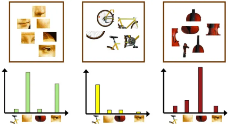
In Table 1, we show the top-5 object classes according to the value of PCA and ICA components. For the ease of comparison, we selected each PCA or ICA component which has the largest value for class mosque, killer whale, Model T or zebra among all components. We can see that the class labels ranked by ICA components are more visually similar than the ones by PCA components.

The PCA/ICA components can be interpreted as common features shared by vi-sually similar object classes. From Figure 26 and Table 1, we can see the label embeddings of object classes by PCA/ICA components are meaningful since vi-sually similar classes are close in the embeddings. Unlike [APHS13], these label embeddings can be unsupervisedly learned with a CNN trained with only one-hot class labels and without any hand annotated attribute label of the object classes, such as has tail or lives in the sea.

The visual-semantic similarity relationship was previously explored in [DF11], which shows some consistency between two similarities. Here we further explore it from another perspective. We dene the visual and the semantic similarity in the following way. The visual similarity between two object classes is dened as cosine similarity of their PCA or ICA components (200-dim and learned with softmax), both of which

(41)

0 10 20 −0.02 0 0.02 0.04 Border terrier 0 10 20 −0.02 0 0.02 0.04

Kerry blue terrier

0 10 20 −0.02 0 0.02 0.04 Irish terrier 0 10 20 −0.05 0 0.05 trolleybus 0 10 20 −0.05 0 0.05 minibus 0 10 20 −0.05 0 0.05 sports car (a) PCA 0 10 20 0 0.02 0.04 0.06 Border terrier 0 10 20 0 0.02 0.04 0.06

Kerry blue terrier 0 10 20 0 0.02 0.04 0.06 Irish terrier 0 10 20 −0.15 −0.1 −0.05 0 trolleybus 0 10 20 −0.15 −0.1 −0.05 0 minibus 0 10 20 −0.15 −0.1 −0.05 0 sports car (b) ICA

Figure 27: Bar plots of PCA/ICA components of object classes. Dimensionality was reduced to 20 for better visualization.

(42)

give the same results. The semantic similarity is dened based on the shortest path length 29 _{between two classes on the WordNet graph [Fel98]. In Table 2, we}

compare ve closest classes of Egyptian cat, soccer ball, mushroon and red wine in terms of visual and semantic similarity. For Egyptian cat, both visual and semantic similarities give similar results. For soccer ball, the visual similarity gives football helmet which is quite distant in terms of semantic similarities. For mushroom and red wine, two similarities give very dierent closest object classes. The gap between two similarities is intriguing and therefore worth further exploration. In neuroscience literature, it is claimed that visual cortex representation favors visual rather than semantic similarity [BANP+_13].

3.3 Learning Semantic Features with MDS

ForW(2) _and_W(3)_{, we use the feature vectors by running classic Multi-dimensional}

Scaling (MDS), as introduced in Section 2.2.4, on a distance matrix of both seen and unseen classes. The distance between two classes is measured by one minus the similarity in the last subsection.

We use a new and simple method for obtaining the semantic features of classes, MDS on WordNet. Compare to Word2Vec on Wikipedia, this avoid three problems: (1) Word ambiguity. There are words which have multiple meanings and represent multiple classes. For example, there are two classes in ImageNet both named y. One means the insect and the other means the shermen's lure. (2) Multiple annota-tions. There are several classes which have multiple annotaannota-tions. For example, class lesser panda, red panda, panda, bear cat, cat bear, Ailurus fulgens. With Word2Vec on Wikipedia, one would obtain multiple feature vectors for these classes. This is no principled way of selecting or combining them. (3) Heavy computation. Typically, Word2Vec on Wikipedia consumes a large amount of RAM and takes hours for com-putation. While classic MDS on the WordNet distance matrix of size 21842×2184230

is much cheaper to compute. The computation of a 21632-dimensional MDS feature vector for each class was done in MATLAB with 8 Intel Xeon 2.5GHz cores within 12 minutes. A comparison of dierent semantic features of classes for zero-shot learn-ing can be found in [ARW+15]. However, MDS on WordNet was not compared in 29_{computed with the path_similarity() function in the NLTK tool http://www.nltk.org/} howto/wordnet.html

30_{21841 classes in ImageNet 2011fall plus class teddy, teddy bear. Class teddy, teddy bear} (Word-Net ID: n04399382) is in Image(Word-Net ILSVRC2012 but not in Image(Word-Net 2011fall.

(43)

[ARW+_{15] (only the raw WordNet distance matrix) and is a part of the contribution}

of this thesis.

3.4 Learning Visual-Semantic Common Space with CCA

Due to the visual-semantic similarity gap shown in the above, we learn a common space between the visual and the semantic representations of object classes via CCA, as introduced in Section 2.2.5, which seeks two projection matrices P(1) and P(2) such that min P(1)_,_P(2)kP (1)T F−P(2)TW(2)kF (61) s.t. P(k)TCkkP(k) =I, p (k)T i Cklp (l) j = 0, (62) k, l= 1,2, k 6=l, i, j = 1, ..., d, (63)

where p(_ik) is the i-th column of P(k) and _C

kl is a covariance or cross-covariance matrix of {f1, ...,fn} and/or{w (2) 1 , ...,w (2) n }.

After projecting the visual features F and the semantic features W(2) _{into a}

com-mon space, the similarity comparison between images from the seen and the unseen becomes more sensible.

3.5 Experiments

Following the zero-shot learning experimental settings of DeViSE and conSE, we used a CNN trained on ImageNet ILSVRC2012 (1000 seen classes), and test our method to classify images in ImageNet 2011fall (20842 unseen classes 31_{, 21841}

both seen and unseen classes). We use top-k accuracy (also called at hit@k in

[FCS+_{13, NMB}+_{14]) measure, the percentage of test images in which a method's}

top-k predictions return the true label.

The CNN model we used is GoogLeNet. The sizes of the matrices in our methods: W(1) is k×1000, W(2) is 21632×1000, W(3) is 21632×20842, P(1) is k × k, P(2) is k×21632, M is 1000×1000 and x is 1000×1. We used k = 100,500,900 in our experiments. Although W(2) _and _W(3) _{are large matrices, we only need to compute}

once and store P(2)_W(2) _and _P(2)_W(3) _{of size} _k_×_{1000 and} _k_×_{21632, respectively.} 31_{The class teddy, teddy bear is missing in ImageNet 2011fall, the correct number of classes is} 21841−(1000−1) = 20842 rather than 20841.

(44)

In Table 3, we show the results of dierent methods on ImageNet 2011fall. We compared random semi-orthogonal, PCA and ICA matrices as the visual features. Our method performs better when using PCA or ICA for the visual features than random features. And our method with random, PCA, or ICA features, achieves the state-of-the-art records on this zero-shot learning task.

In Table 4, we show the results of dierent methods on ImageNet ILSVRC2012 validation set of 1000 seen classes. While the goal here is not to classify images of seen classes, it is desirable to measure how much accuracy a zero-shot learning method would lose compared to the softmax baseline. Again, we can see that our method performs better using PCA or ICA for the visual features than random features.

In Table 5, we show the results of the three zero-shot learning methods on the test images selected in [NMB+14]. Same as conSE, our method gives correct or

reasonable predictions. The correct labels are in blur color.

Table 3: Top-k accuracy in ImageNet 2011fall zero-shot learning task (%).

Test Set #Classes #Images Method Top-1 Top-2 Top-5 Top-10

DeViSE (500-dim) 0.8 1.4 2.5 3.9

ConSE (500-dim) 1.4 2.2 3.9 5.8

Our method (100-dim, random) 1.4 2.2 3.4 4.3

Our method (100-dim, PCA) 1.6 2.7 4.6 6.4

Our method (100-dim, ICA) 1.6 2.7 4.6 6.3

Unseen 20842 12.9 million Our method (500-dim, random) 1.8 2.9 5.0 6.9

DeViSE (500-dim) 0.3 0.8 1.9 3.2

ConSE (500-dim) 0.2 1.2 3.0 5.0

Both 21841 14.2 million Our method (500-dim, random) 6.7 8.5 11.2 13.4

32_{WordNet ID: n02077152. There are two classes named fur seal with dierent WordNet IDs.} 33_{WordNet ID: n02077658.}

(45)

Table 4: Top-k accuracy in ImageNet ILSVRC2012 validation set (%).

Test Set #Classes #Images Method Top-1 Top-2 Top-5 Top-10

Softmax baseline (1000-dim) 55.6 67.4 78.5 85.0

DeViSE (500-dim) 53.2 65.2 76.7 83.3

ConSE (500-dim) 54.3 61.9 68.0 71.6

Our softmax baseline (1000-dim) 67.1 78.8 87.9 92.2

Seen 1000 50000 Our method (100-dim, ICA) 67.0 76.9 84.6 88.5

Table 5: Predictions of test images of unseen classes (correct class labels are in blue)

Test Images DeViSE ConSE Our Method

water spaniel business suit periwig

tea gown dress mink

bridal gown hairpiece tights

spaniel swimsuit quack-quack

tights kit horsehair wig

heron ratite ratite

owl peafowl kiwi

hawk common spoonbill moa

bird of prey New World vulture elephant bird

nch Greek partridge emu

elephant California sea lion fur seal32

turtle Steller sea lion eared seal

turtleneck Australian sea lion fur seal33

ip-op South American sea lion guadalupe fur seal

handcart eared seal Alaska fur seal

golden hamster golden hamster golden hamster

rhesus rodent Eurasian hamster

pipe Eurasian hamster prairie dog

shaker rhesus skink

American mink rabbit mountain skink

truck, motortruck atcar skidder

skidder truck bulldozer

tank car tracked vehicle farm machine

automatic rie bulldozer cultivator

trailer wheeled vehicle angledozer

kernel dog masti

littoral domestic cat Seeing Eye dog

carillon schnauzer guide dog

Cabernet Belgian sheepdog alpaca

(46)

3.6 Discussion

The results of our experiments show that in our method the PCA or ICA matrix as visual features of object classes performs better than a random matrix. Therefore, these visual features, learned by PCA and ICA on the outputs of CNN, are indeed eective for the subsequent tasks. The results also show that PCA and ICA give the essentially same classication accuracy. Therefore, in practice we can use PCA instead of ICA, which has much higher computational costs. For a more compre-hensive discussion on PCA vs. ICA for recognition tasks, see [AVHH07].

4 Conclusions

The outputs of a neural network contains rich information. It has been claimed that one can determine a neural network architecture by observing its outputs given arbitrary inputs [FM94]. Also, it has been shown that one can reconstruct the whole image to some degree with only its CNN outputs [DB15]. And smooth regularization on the output distribution of a neural network can help in reducing generalization error in both supervised and semi-supervised settings [MMK+_15].

CNN achieves the state-of-the-art results on many computer vision tasks such as image classication and object detection. However, despite many eorts of visual-izing and understanding CNN [ZF14, SVZ14, ZKL+15], it still reminds a black-box

method. In this thesis, we attempted to understand CNN by unsupervised learning. CNN was trained with only one-hot targets, which means we assumed object classes are equally similar. We never told CNN which classes more similar. But unsuper-vised learning on CNN outputs reveals the visual similarity of object classes. We hope this nding can shed some lights on the object representation in CNN.

We also showed that there is a gap between the visual similarity of object classes in CNN and the semantic similarity of object classes in our knowledge graph. There-fore, a bridge should be built, in order to achieve consistent mapping between visual and semantic representations.

Supervised learning alone cannot deal with unseen classes since there is no training data. By using external knowledge and unsupervised learning algorithms, we can leverage supervised learning so as to make reasonable predictions on the unseen classes while maintaining the compatibility with the seen classes, that is, zero-shot learning. In this thesis, we proposed a new zero-shot learning method, which achieves