A mechanistic model for the negative binomial distribution of single-cell mRNA counts

Graphical Abstract

A mechanistic model for the negative binomial distribution of single-cell mRNA counts Lisa Amrhein, Kumar Harsha, Christiane Fuchs

Biological Process Estimation & Parameter Selection Prediction Data # # Frequency Frequency Knowledge Transfer Simplification

Mechanistic Model Steady State Distribution

Li n k vi a O rn st ei n -U h le n b ec k p ro ce ss es

#

~

#

~

#

~

A mechanistic model for the negative binomial distribution of single-cell

mRNA counts

Lisa Amrheina,b_{, Kumar Harsha}a,b_{, Christiane Fuchs}a,b,c,d,∗

a_{Institute of Computational Biology, Helmholtz Zentrum Munich, 85764 Neuherberg, Germany} b_{Department of Mathematics, Technical University of Munich, 85747 Garching, Germany} c_{Faculty of Business Administration and Economics, Bielefeld University, 33615 Bielefeld, Germany}

d_{Lead Contact}

Summary

Several tools analyze the outcome of single-cell RNA-seq experiments, and they often assume a probability distribution for the observed sequencing counts. It is an open question of which is the most appropriate discrete distribution, not only in terms of model estimation, but also regarding interpretability, complexity and biological plausibility of inherent assumptions. To address the question of interpretability, we inves-tigate mechanistic transcription and degradation models underlying commonly used discrete probability distributions. Known bottom-up approaches infer steady-state probability distributions such as Poisson or Poisson-beta distributions from different underlying transcription-degradation models. By turning this procedure upside down, we show how to infer a corresponding biological model from a given probability distribution, here the negative binomial distribution. Realistic mechanistic models underlying this distribu-tional assumption are unknown so far. Our results indicate that the negative binomial distribution arises as steady-state distribution from a mechanistic model that produces mRNA molecules in bursts. We empirically show that it provides a convenient trade-off between computational complexity and biological simplicity.

Keywords: gene expression, negative binomial distribution, Poisson-beta distribution, single-cell RNA sequencing, switching process, bursting process, stochastic differential equation, Ornstein-Uhlenbeck process

Introduction

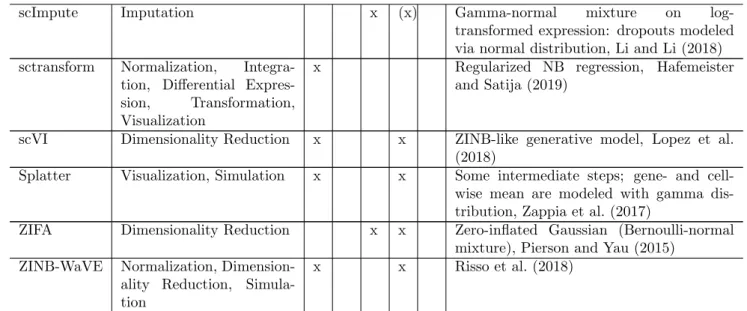
When analyzing the outcomes of single-cell RNA sequencing (scRNA-seq) experiments, it is essen-tial to appropriately take properties of the result-ing data into account. Many methods assume a parametric distribution for the sequencing counts due to its larger power than non-parametric ap-proaches. To that end, a family of parametric dis-tributions which adequately models the data needs to be chosen. In Supplementary Table S1, we pro-vide an overview of computational tools for scRNA-seq analyses and their distribution choices. Among

∗_{Correspondence} Email address:

[email protected](Christiane Fuchs)

the 23 listed tools, around 60% use a negative bi-nomial (NB) distribution, 40% a zero-inflated dis-tribution (these two cases can overlap) and about 7% a Poisson-beta (PB) distribution.

Count data is most appropriately described by dis-crete distributions unless count numbers are with-out exception very high. A commonly chosen dis-tribution is the Poisson disdis-tribution, which can be derived from a simple birth-death model of mRNA transcription and degradation. However, due to widespread overdispersed data, it is sel-dom suitable. Another typical choice is a three-parameter PB distribution (Delmans and Hemberg, 2016, Vu et al., 2016) which can be derived from a DNA switching model (also called random tele-graph model, see Dattani and Barahona, 2017, or

basic model of gene activation and inactivation, see Raj et al., 2006). Parameters of the PB

distribu-tion can be estimated from scRNA-seq data (Kim and Marioni, 2013), as well as experimentally mea-sured and inferred (Suter et al., 2011). This distri-bution provides good estimates of scRNA-seq data; however, it entails the estimation of three param-eters which introduces a high computational cost (Kim and Marioni, 2013). A frequent third choice is the NB distribution, used by several tools that analyze single-cell gene expression measurements such as SCDE (Kharchenko et al., 2014), Mono-cle 2 (Qiu et al., 2017) and many more (see Sup-plementary Table S1). This distribution is chosen due to computational convenience and good empir-ical fits. Mathematempir-ically, it can be considered as asymptotic steady-state distribution of the switch-ing model (see Raj et al., 2006). However, this will entail biologically unrealistic assumptions. So far, no mechanistic model is known that directly leads to a NB distribution in steady state.

To close this gap, we look again at the already known mechanistic processes and their inferred parametric steady-state distributions: Poisson and PB. Integrating these in the general framework of Ornstein-Uhlenbeck (OU) processes (Barndorff-Nielsen and Shephard, 2001), we aim to transfer a general method of connecting mechanistic pro-cesses via stochastic differential equations (SDEs) and their theoretical steady-state distributions to this research problem. Hence, we show how to con-nect a desired steady-state distribution of the in-tensity process with the corresponding SDE by us-ing OU processes and their properties. We use this method to calculate the corresponding SDE from the NB distribution as given steady-state distribu-tion; from this, we can read a corresponding mech-anistic model. In a (Case Study), we use our R packagescModelsto estimate three count distribu-tion models (Poisson, PB and NB) on simulated perfect-world data, and perform model selection as well as goodness-of-fit tests. A comparison with ex-isting implementations of the PB distribution, de-tailed derivations and definitions of the employed probability distributions can be found in the Ap-pendix. Lastly, we repeat this comparison on real-world data and extend the models to more realistic ones by including zero inflation and heterogeneity. By inferring a mechanistic model for stochastic gene expression, our work validates the NB distribution as a steady-state distribution for mRNA content in single cells.

A

B

C

D

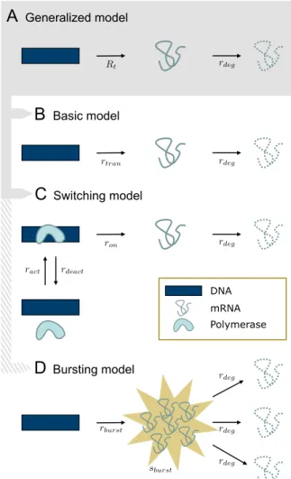
Figure 1: Transcription and degradation models: (A) Gen-eralized model with time-dependent stochastic transcription rate Rt and constant deterministic degradation rate rdeg.

(B) Basic model with constant deterministic transcription and degradation rates. (C) Switching model of gene acti-vation and inactiacti-vation, transcription and degradation. (D) Bursting model, where bursts occur at raterburst and burst

sizes have mean sburst. This model differs from (A) in

that transcription events can produce more than one mRNA molecule.

Results

It has previously been shown how to derive an mRNA count distribution from a simple birth-death model for mRNA transcription and degra-dation (Dattani and Barahona, 2017, Peccoud and Ycart, 1995). Alterations in the transcription and degradation model lead to alterations in the re-sulting mRNA count distribution. We will sketch the derivation of several such models and distribu-tions. Our models describe the number of mRNA molecules in a cell for eitheronegene or for a group

of genes for which we can assume identical kinetic parameters.

In the general context, we consider a transcription-degradation model with stochastic time-varying transcription rate Rt and deterministic constant degradation rate rdeg (Figure 1A). Here, the num-ber of mRNA molecules at time t is Poisson dis-tributed with intensityItfollowing the random dif-ferential equation

dIt=−rdegItdt+Rtdt (1) fort≥0 and fixed I0=i0 >0. Depending on the transcription process, described by Rt, this RDE has different solutions which will be shown in the following (for detailed calculations see Appendix). Basic model: constant transcription and degradation. In the basic model, transcrip-tion and degradatranscrip-tion occur at constant ratesrtran

andrdeg (Figure 1B). The RDE (1) simplifies to the ordinary differential equation (ODE)

dIt=−rdegItdt+rtrandt (2)

with time-independent non-stochastic steady state

It = rtran/rdeg. Hence, if the cell is in steady

state, mRNA counts in this model follow a Poisson distribution with constant intensityrtran/rdeg (see Appendix).

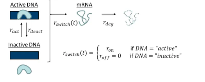
Switching model: gene activation and deacti-vation. In the well-knownswitching model, a gene switches between an inactive state where transcrip-tion is impossible, and an active state where tran-scription occurs. This can be explained by poly-merases binding and unbinding to the specific gene (Figures 1C and S1). The RDE (1) becomes

dIt=−rdegItdt+rswitch(t)dt (3)

with

rswitch(t) =

(

ron if DNA active at timet roff if DNA inactive at time t, whereroff < ron. The transcription rate is modeled

by a continuous-time Markov process (rswitch(t))t≥0 that switches between two discrete states ron

androff with activation and deactivation ratesract

andrdeact, respectively. One usually sets roff = 0.

This corresponds to a system where a gene’s en-hancer sites can be bound by different tion factors or co-factors. Once bound, transcrip-tion occurs at constant rate ron, and mRNA con-tinuously happens at constant rate rdeg. Waiting

times between switches are assumed to be exponen-tially distributed. As shown in the Appendix, these assumptions lead to It following a four-parameter Beta (ract/rdeg, rdeact/rdeg, roff/rdeg, ron/rdeg) dis-tribution, and therefore the mRNA content in steady state is described by a Poisson-beta (PB) distribution. Hence, the probability of

hav-ing n mRNA molecules at time t is

time-independent. For roff = 0 (i. e. no transcription possible during inactive DNA state), it can be sim-plified to P(n, t) = Γract rdeg + rdeact rdeg ron rdeg n Γract rdeg +n Γract rdeg Γ(n+ 1)Γract rdeg + rdeact rdeg +n ×1F1 _ract rdeg +n,rdeact rdeg +ract rdeg +n,−ron rdeg , (4)

where Γ denotes the gamma function and

1F1(a, b, z) = _{Γ(a)Γ(b−a)}Γ(b) R

1 0 e

zu_ua−1_(1−u)b−a−1_du is the confluent hypergeometric function of first order, also called Kummer function. The density function of this PB distribution converges to the density function of a negative binomial (NB) distribution under specific conditions (Appendix).

For ron = rtran, ract → ∞ and rdeact = 0, the

switching model reduces to the basic model, and the above PB distribution collapses to a Poisson distribution with intensity parameterrtran/rdeg, in

consistency with the above-derived results.

Connecting SDEs with steady-state distribu-tions. Taken together, both models described the intensity process of a Poisson distribution (Equa-tions 2 and 3). These intensity processes govern the transcription and degradation within the mechanis-tic models. They determine the steady-state dis-tribution of the intensity parameter, and thus the overall distribution of the mRNA content. Impor-tantly, changes in the intensity process lead to dif-ferent steady-state distributions. We generalize this framework by using Ornstein-Uhlenbeck (OU) pro-cesses and their properties (Barndorff-Nielsen and Shephard, 2001).

The general definition of an OU SDE (adjusted to the above notation) is given by

dIt=−rdegItdt+ dLt, (5) whereLtwithL0= 0 (almost surely) is a L´evy pro-cess, i. e. a stochastic process with independent and

stationary increments. In addition, we needLt to be a subordinator, that is a L´evy process with pos-itive increments (Definition 7 in Appendix). A spe-cial property of OU processes is that, under certain conditions (see Definition 9), for a chosen distribu-tionDthere is an OU process that in steady state leads to this distribution D. The other direction, i. e. the existence of a steady-state distribution D for a chosen OU process (in terms of its subordi-nator), holds as well. For a given L´evy subordina-torLt, the characteristic function ofD, and thusD itself, can be derived as described in the following (adjusted to the notation of Equation 5):

1. Find the characteristic function ˆµLt(z) of the

L´evy subordinatorLt.

2. Calculate ˆµL1(z) and write the result in the

form exp(φ(z)) for some functionφ(z). 3. Calculate the characteristic function C(z) of

the stationary distributionD of It by setting

C(z) = exp(r−1_degRz

0 φ(ω)ω

−1_{dω). C(z) leads} toD.

More details and examples are shown in the Appendix. Despite this apparently clear line of action, finding a corresponding law D and processLtis challenging without prior knowledge, e. g. ifD is not well-known or Lt is only specified through the characteristic function of L1. In the next section, we cast the NB distribution as an alternative distribution for which a subordinator can be derived.

Negative binomial distribution: Deriving an explanatory bursting process. A widely con-sidered model for scRNA-seq counts is the NB dis-tribution. Like the above-employed PB distribu-tion, it accounts for overdispersion by modeling the variance independently of the mean of the data. Having one parameter less than PB, NB is an ap-pealing choice. However, mechanistic models derlying the NB distributional assumption are un-known. We aim to derive such a mechanistic model of transcription and degradation by reversing the steps that led from the switching model to the PB distribution. For that purpose, an important fact is that an NB distribution can be expressed as a Poisson-gamma (PG) distribution, i. e. as a condi-tional Poisson distribution with gamma distributed intensity parameterI. One has

PG(α, β) ˆ= NB α,(β+ 1)−1 (6)

forα, β >0 as derived in the Appendix.

In analogy to the derivation of the PB distribution from the switching model, we now seek to describe the mRNA content by a Poisson distribution with intensity parameter It, which in steady state fol-lows a gamma distribution instead of a beta dis-tribution. Thus, we aim to specify an OU process with the gamma distribution as steady-state dis-tribution. In terms of mechanistic modeling, this means that we need to describe a suitable tran-scription process. Mathematically, we need to spec-ify the L´evy subordinatorLt accordingly. From fi-nancial mathematics it is known that a stationary gamma distribution is obtained if Lt is chosen to be a compound Poisson process (CPP, see Defini-tion 8) with exponentially distributed jump sizes (Barndorff-Nielsen et al., 2001). This will be our choice of subordinator; however, the parameters of this process still need to be specified. In the follow-ing, we will show that the L´evy subordinator of the OU process (5) whose one-dimensional stationary distribution is Gamma(α, β), is a CPP with inten-sity parameterα·rdeg and mean jump sizeβ−1. To obtain this result, we follow the three-step pro-cedure described above in reverse order. We start with D= Gamma(ˆ α, β) and transform its charac-teristic function to expnr_deg−1 Rz

0 φ(ω)ω

−1_dωo_{, using} the characteristic function ofDas given in the Ap-pendix, Definition 1: C(z) = 1−iz β −α = exp −αlog 1−iz β = exp α Z z 0 −1 iβ+ωdω = exp α Z z 0 iω (β−iω)ωdω = exp r_deg−1 Z z 0 α rdeg _β β−iω −1 ω−1dω = exp r_deg−1 Z z 0 φ(ω)ω−1dω

withφ(ω) =α rdeg_β−iωβ −1andithe imaginary

number. Next, we use ˆµL1(z) = exp(φ(z)) to obtain

ˆ µL1(z) = exp α rdeg _β β−iz−1 . (7)

We aim to bring this into agreement with ˆµLt(z),

the time-dependent characteristic function of a gen-eral CPP Lt with intensity parameter λ. This is

given by ˆ

µLt(z) = exp(t λ(ˆµY(z)−1)),

whereY is a random variable following the distribu-tion of the jump sizes of the CPP, and ˆµY is its char-acteristic function (see Appendix, Definition 8). A CPP with intensity λ = α·rdeg and i.i.d. expo-nentially distributed incrementsY ∼Exp(β) with characteristic function ˆµY(z) = β/(β−iz) yields the overall characteristic function

ˆ µLt(z) = exp tαrdeg _β β−iz −1 .

This is in accordance with ˆµL1(z) as derived in

Equation (7), and hence, a mathematically appro-priate subordinator is a CPP with intensity param-eterα·rdeg and mean jump sizeβ−1.

As a consequence, transcription is expressed via a stochastic processLt, namely the CPP, which expe-riences jumps after exponentially distributed wait-ing times. In contrast to the L´evy subordinators of the basic model,Lbasic_t =ront, and of the switching model,Lswitcht =

Rt

0rswitch(s)ds, it possesses point-wise discontinuous sample paths (Figure 2, right). Intervals without any transcription activity seem to be disrupted by sudden explosions of mRNA num-bers. This burstiness led us to call the mechanism behind the NB distribution thebursting model. We denote its subordinator byLburst

t and argue the bi-ological justification of the model in the Discussion and Conclusion.

We aim to derive the mechanistic transcription pro-cess of the bursting model in more detail. Specif-ically, we tackle the distribution of burst sizes of mRNA counts. For this we look at a heuristic tran-sition fromLswitch

t toLburstt .

First, we dismantle the shape of the trajectories ofLswitcht . As depicted in Figure 2 on the left, such a trajectory consists of alternating piecewise con-stant and piecewise linear parts. The concon-stant parts appear during time intervals without transcription, i. e. where the DNA is inactive. The length of such a time interval depends only on the rateract of the

switching model. Once the DNA switches into the active mRNA transcribing state, the time interval with transcription depends only on the raterdeact. The slope of the trajectory during this active DNA state represents the transcription strength and de-pends only on the parameterron.

In case the length of the time interval of active DNA becomes infinitesimally small, and at the same time

the transcription strength becomes infinitesimally large, the trajectory of Lswitch

t turns into a step

function as depicted in Figure 2 on the right. This limit is obtained if rdeact → ∞ and ron → ∞ in a way that needs to be specified. For that reason, we in the following seek to describe a mechanistic model for the transition phase (Figure 2, middle) leading to the bursting model.

In the switching model, as soon as DNA becomes active, a competition starts between the events

transcription and deactivation. In addition, degra-dation may happen, which will affect the intensity process It and the number of mRNA molecules, but not the transcription process. If a transcrip-tion event occurs, the competitranscrip-tion between tran-scription and deactivation continues at the same probability rates as before; the only affected event probability is the one for degradation because this probability depends on the current mRNA count. We now consider the following approximation of the switching model and call it the transition model: When DNA becomes active, we allow the events transcription and deactivation to happen, but not degradation. To correct for the missing degrada-tion events, we introduce a waiting time W after DNA deactivation in which only degradation can occur, but no DNA activation. For appropriately chosen rdeact → ∞ andron → ∞, the

approxima-tion error will tend to zero.

The number of transcription events S during one active DNA phase is geometrically distributed with success probability parameterrdeact/(rdeact+ron).

In the interpretation of the geometric distribution, transcription events are considered as failures, de-activation as success. The waiting timeW needs to accumulate the times before S transcriptions and one deactivation. Thus, W = T1+· · ·+TS +D, where Ti ∼ Exp(ron), i = 1, . . . , S, are the sin-gle waiting times for each transcription event and

D ∼ Exp(rdeact) is the waiting time till the next

DNA deactivation.

Taken together, the bursting process can be con-sidered as the limiting process of the approxima-tion of the switching process as ron → ∞ and

rdeact → ∞ under the condition that the success

probability parameter of the geometric distribution,

rdeact/(rdeact+ron) stays constant. As the link

be-tween the switching model and PB distribution is known, and since PB converges towards NB under certain conditions (see Appendix), we can connect the parameters of the bursting model with those of the NB distribution and CPP.

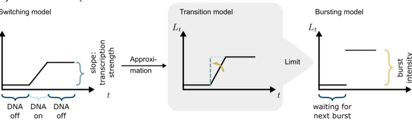
Switching model Bursting model Lévy Subordinators Limit DNA off DNA on slope: tr anscr ipti on strength Approxi-mation DNA off waiting for next burst burst intensit y Transition model

Figure 2: The L´evy subordinator of the switching model is shown on the left by means of an exemplary trajectory. For small duration of the DNA being active and large transcription strength, its behavior can be approximately described by a step function as depicted in the middle (transition model). The limit of this approximation, with infinitesimally small DNA activation time interval and infinitesimally large transcription strength, leads to a trajectory of the subordinator of the bursting model which is shown on the right.

That is, the bursting model can mechanistically be described as follows: After Exp(rburst)-distributed waiting times, a Geo((1 + sburst)−1)-distributed number of mRNAs are produced at once, where

sburst is the mean burst size (see also Golding

et al., 2005). As in the basic and switching models, degradation events occur with Exp(rdeg

)-distributed waiting times. The just described mech-anistic bursting model is shown in Figure 1D. It can equivalently be described by the OU process (5) with Lt being a CPP with Exp(rburst)-distributed

waiting times and Exp(sburst)-distributed jump sizes. Thus, in steady state, mRNA counts follow a

PG(rburst/rdeg, sburst) distribution or, equivalently,

a NB rburst/rdeg,(1 +sburst)−1

distribution if the bursting model is assumed.

The NB rburst/rdeg,(1 +sburst)−1

model, again, can be interpreted as follows (see also Appendix, Definition 3): Assume you have an empty bucket into which you put balls according to the follow-ing stochastic procedure. You perform a number of independent Bernoulli trials, each with success probability (1 +sburst)−1. If there is a failure, you

add one ball to the bucket. If there is a success, you do not do anything but count the success event. You continue until there have beenrburst/rdeg

suc-cesses. (For interpretation purposes, we here

as-sume rburst/rdeg to be a whole-valued number.)

The larger sburst, the smaller the success proba-bility, i. e. by expectation you will put more balls in the bucket for largesburst. Similarly, the larger the ratio ofrburst to rdeg, the more success events will be waited for, thus the more balls will tend to

be added. The final number of balls in the bucket represents the number of mRNA molecules in a cell at steady state.

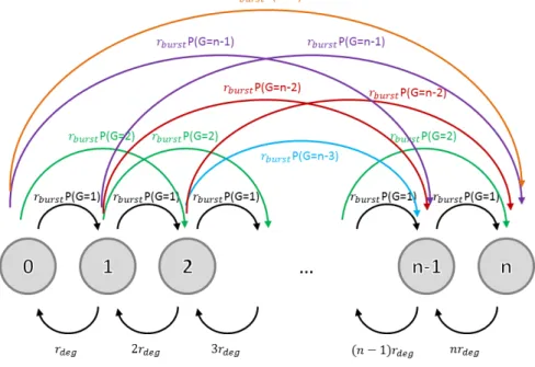
The above top-down derivation from the steady-state distribution to the mechanistic process has to be motivated heuristically in parts. In the Appendix we prove bottom-up that the above described mechanistic bursting model indeed leads to the steady-state NB distribution by directly calculating the master equation (see also Supple-mentary Figure S2).

Heterogeneity and dropout. The transcription and degradation models considered so far describe the number of mRNA molecules for homogeneously expressed genes that are actually present in a cell. Real-world data is usually more complex: First, cell populations may be heterogeneous. Second, scRNA-seq measurements will be subject to mea-surement error. For example, they often contain a large number of zeros. If a zero is due to techni-cal error, it is techni-called dropout. Regardless of what causes this phenomenon, a data model should take this property into account. We describe two model extensions here.

Data that originates from different cell populations (in terms of different transcriptomic properties) can be modeled mathmatically. If a population consists of e. g. two subpopulations, each of them is mod-eled by one single distribution, D1 or D2, parame-terized via θ1 and θ2, respectively. One assumes the mRNA count to be distributed according to

With probability p, the count distribution of that cell is D1, otherwise D2. The corresponding mix-ture density is given by

f2mix(x;θ1, θ2, p) =p f1(x;θ1) + (1−p)f2(x;θ2), where f1 and f2 are the densities of D1 and D2, and x is the observed mRNA count. For k > 2 subpopulations, the density can easily be general-ized to a mixture ofkdistributionsD1, . . . ,Dkwith probabilitiesp1, . . . , pk: fkmix(x;θ1,· · ·, θk, p1,· · ·, pk−1) = (8) p1f1(x;θ1) +. . .+ 1− k−1 X i=1 pi ! fk(x;θk).

The distributions Di can be any (ideally discrete count) distribution, possibly from different distri-bution families.

An appropriate model for the occurrence of the above-mentioned dropout is a zero-inflated distri-bution (Kharchenko et al., 2014). For one homo-geneous population, the mRNA count will be dis-tributed according top_1{0}+(1−p)D(θ), with_1{0} being the indicator function with point mass at zero, and the corresponding density function reads

fzi(x;θ, p) =p1{0}(x) + (1−p)f(x;θ), wheref is the density function of D. Analogously, zero inflation can be added to a mixture of several distributions, see (8). mRNA counts are then dis-tributed according to p_11{0}+p2D1(θ1) +. . .+ 1− k X i=1 pi ! Dk(θk). The corresponding density function is given by

fzi-kmix(x;θ1,· · ·, θk, p1,· · ·, pk) = p11{0}(x) +p2f1(x;θ1) +. . . + 1− k X i=1 pi ! fk(x;θk).

Data application. We perform a comprehensive comparison of the considered mRNA count distri-butions, that is the Poisson, NB and PB distribu-tion, when applied to real-world data. Within each of the three distributions we further consider mix-tures of two populations (from identical distribu-tion types but with different parameters) with and

without additional zero inflation. In total, we in-vestigate twelve different models as shown in Fig-ure 3. The numbers of parameters in these models are listed in Supplementary Table S3.

0 1,251 43 1,294 1,045 2 1,043 0 1 7,248 159 7,408 428 0 427 1 2 9,969 204 10,175 1-pop ZI-1-pop ZI-2-pop 2-pop Pois NB PB

A

B

Selected distributions after GOF

1,000 100 0 10,000 100 0

Figure 3: Frequencies of chosen distributions via BIC-after-GOF applied to real-world datasets: (A) Nestorowa et al. (2016) (B) mm10:10x, Official 10x Genomics Support (2017).

We estimate these twelve models on two real-world datasets: The first one stems from Nestorowa et al. (2016), contains 1,656 mouse HSPCs and was generated using the Smart-Seq2 (Picelli et al., 2014) protocol, and thus did not employ unique molecular identifiers (UMIs). The second dataset contains 3,356 homogeneous NIH3T3 mouse cells and has been generated using the 10x Chromium technique (Zheng et al., 2017), thus incorporat-ing UMIs. It is part of the publicly available 10x dataset “6k 1:1 Mixture of Fresh Frozen Human (HEK293T) and Mouse (NIH3T3) Cells” (Official 10x Genomics Support, 2017). Here, we refer to this dataset asmm10:10x.

We applied a gene filter (see Appendix), estimated the model parameters of the twelve considered models via maximum likelihood, and performed model selection as described in the Case Study via

the Bayesian information criterion (BIC). Figure 3 summarizes the frequencies of the chosen models across genes. We only display those choices where the chosen distribution with estimated parameters was not rejected by a goodness-of-fit (GOF) test (χ2_{-test) at 5% significance level with multiple} test-ing correction.

In the data from Nestorowa et al. (2016), 16,364 genes remained after filtering, of which 10,175 were not rejected by the GOF test. Figure 3A shows that some variant of the NB distribution was chosen for 98% of these genes. Among these, mRNA count numbers for many genes were best described by the zero-inflated NB distribution. However, an even higher preference could be observed for the mixture of two NB distributions. This can be explained by taking a closer look at the gene expression counts of the affected genes (see also Supplementary Fig-ure S6): Most of those genes not only show many zeros, but also many low non-zero counts, i. e. many ones, twos etc., next to higher counts. Such ex-pression profiles are not covered by a simple zero-inflated model but prefer a mix of two distributions, one of them mapping to low expression values (see Supplementary Table S3).

In the mm10:10x data, 4,203 genes remained after filtering and the GOF test. Figure 3B shows that for 89% of these genes, an NB distribution vari-ant was chosen as most appropriate model. How-ever, other than for the dataset from Nestorowa et al. (2016), the standard NB distribution (for one population, without zero inflation) was sufficient in the majority of cases. We looked for commonali-ties between the gene profiles that led to the same distribution choice. Supplementary Figure S5 sug-gests an interdependence between the chosen one-population distributions and the range of the pa-rameter estimates.

Taken together, the NB distribution was chosen for most gene profiles, either as a single distribution, a mixture of two NB distributions or with additional zero inflation.

NB distribution as commonly chosen count model. While the mechanistic models and their steady-state distributions describe actual mRNA contents in single cells, real-world data underlies technical variation in addition to biological com-plexity. We investigated in a simulation study (Case Study and Figure 4) and on real-world data (Figure 3) which distributions were most appropri-ate among those considered to describe gene

expres-sion profiles. The simulation study showed that an NB distribution may be best suited even if the in silico data had been generated from the switching model. Also in the real-data application, the NB distribution was chosen in most cases. In line with our expectations, gene profiles of the non-UMI-based dataset by Nestorowa et al. (2016) showed strong preference for a two-population mixture or zero-inflated variant of the NB distribution. In con-trast, the mm10:10x dataset consists by construc-tion of homogeneous cells, and 10x Chromium is not known for large amounts of unexpected zeros in the measurements. Accordingly, the single-population NB distribution was sufficient for most gene profiles here. For 9% of the considered genes in the m10:10x dataset, mRNA counts were most appropriately de-scribed by some form of the Poisson distribution. We have examined these 366 genes for functional similarities; while estimated parameters show some apparent pattern (Supplementary Figure S5), we did not find any defining biological characteristics (Supplementary Figure S7).

Similar to us, Vieth et al. (2017) performed model selection among Poisson, NB and PB distributions by BIC and GOF on several publicly available datasets. Although they used the method of Vu et al. (2016) for which computation of the GOF statistics is impossible for the PB distribution, they still observed a tendency towards the NB distribu-tion as preferred models. In our study, we represent the PB density in terms of the Kummer function, which allows us to compute the GOF statistics ac-cordingly.

Different sequencing protocols might lead to differences in distributions and also might generate data of different magnitudes. Ziegenhain et al. (2017) applied various sequencing methods to cells of the same kind to understand the impact of the experimental technique on the data. Based on the so-generated data, Chen et al. (2018) investigated differences in gene expression profiles between read-based and UMI-based sequencing technolo-gies. They concluded that, other than for read counts, the NB distribution adequately models UMI counts. Townes et al. (2019) suggest to describe UMI counts by multinomial distributions to reflect the nature of the sequencing procedure; for computational reasons, they propose to ap-proximate the multinomial density again by an NB density. Overall, the NB distribution appears sufficiently flexible to hold independently of the specific sequencing approach.

R package scModels. We provide the R pack-age scModels which contains all functions needed for maximum likelihood estimation of the consid-ered distribution models. Three applications of the Gillespie algorithm (Gillespie, 1976) allow synthetic data simulation (as used in the Case Study) via the basic, switching and bursting model, respectively. Implementations of the likelihood functions for the one-population case and two-population mixtures, with and without zero inflation, allow inference of the Poisson, NB and PB distributions. We pro-vide a new implementation of the PB density, based on our novel implementation of the Kummer func-tion, also known as the generalized hypergeomet-ric series of Kummer. This became necessary, be-cause the existing R function (kummerM() con-tained in packagefAsianOptions) was only valid for specific parameter values, and hence, was not suited for optimization in continuous unconstrained space (more information in Appendix). Existing packages such asD3E(Delmans and Hemberg, 2016), imple-mented inPython, andBPSC(Vu et al., 2016), im-plemented inR, use the PB distribution for scRNA-seq data analysis but based on a different approxi-mation scheme (see Appendix). With our new im-plementation of the PB density we did not overcome the problem of time-consuming calculation, but we for the first time provided an implementation of the Kummer function inRvalid for all values required inside the PB density. For a more detailed descrip-tion ofscModelsand a package comparison toD3E andBPSC, see the Appendix.

Case Study

In a simulation study, we generate in silico data from the three considered mechanistic models: the basic model (Figure 1B), the switching model (Fig-ure 1C), and the bursting model (Fig(Fig-ure 1D), using the Gillespie algorithm implemented in scModels. In order to choose realistic values for the rate pa-rameters, we orient ourselves on experimental stud-ies which aim to determine rates of the switching process in specific cases. For example, Suter et al. (2011) identify rates for so-called short-lived genes where mRNA and protein pulses are directly con-nected to one single on-and-off-switch of a gene. We provide an overview of the employed rate combina-tions in Supplementary Table S4.

As a proof of concept, we estimate the three corresponding distributions, i. e. the Poisson, the

Poisson-beta (PB) and the negative binomial (NB) distribution, on all generated datasets via maxi-mum likelihood estimation. To investigate which distribution explains the data best, we compute the Bayesian information criterion

BIC =−2`(θˆ) + log(n)dim(ˆθ),

where`represents the corresponding log-likelihood function, θ the possibly multivariable parameter vector of the distribution, ˆθits maximum likelihood estimate, dim(ˆθ) its dimension, i. e. the number of unknown scalar parameters, andnthe sample size. The distribution with lowest BIC value is consid-ered most appropriate among all considconsid-ered mod-els. Afterwards, we apply a χ2-test to assess the goodness-of-fit (GOF) and neglect those datasets for which the distribution fits are rejected at the 5% significance level (without multiple testing cor-rection). This reduces the total number of 1,000 simulated datasets per model to the amounts dis-played in Figure 4A.

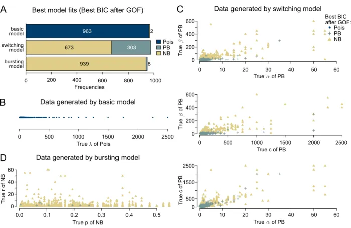
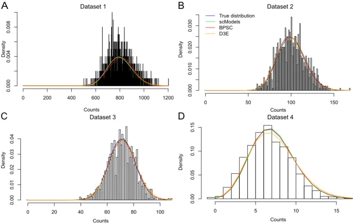
We investigate whether the selected distributions correspond to the distributions that arise from the respective mechanistic models: For the datasets generated from the basic model, model selection via BIC-after-GOF indeed prefers the Poisson dis-tribution in most cases, independently of the used distribution parameterλ(Figure 4A, first bar, and Figure 4B). In contrast, for datasets generated by the switching model, BIC-after-GOF in big parts chooses either the NB or the PB distribution (Fig-ure 4A, middle bar). The choice seems to depend on the employed rate parameters: Figure 4C indicates a tendency towards the PB distribution for low val-ues ofβ; otherwise, the NB distribution often seems to model the data generated by the switching model sufficiently well. For datasets generated by the bursting model, BIC-after-GOF picks the NB dis-tribution for the majority of the time without any obvious bias (Figure 4A/D). The study shows that, apparently, the NB distribution is complex enough to describe the data generated from the switching model. The BIC decides in many cases that a po-tentially better fit is not worth the extra effort for estimating an additional parameter in the PB dis-tribution.

Discussion and Conclusion

In this work, we derived a mechanistic model for stochastic gene expression that results in the NB

PB NB PB NB 939 8 ●●● ●● ● ● ● ●● ● ●● ● ●● ● ● ● ● ●● ● ● ●● ● ●● ● ● ● ●●● ●●● ● ● ● ● ●● ● ● ●● ●●● ●● ●● ● ●● ●● ●● ●● ● ● ●● ● ● ● ● ● ● ● ● ● ●● ●● ● ●● ● ● ●●●● ● ● ● ●● ● ● ● ●●● ● ● ● ● ●● ●●●● ● ●● ●●● ● ● ● ● ●● ●● ● ● ● ● ● ● ● ● ●● ● ●●●● ● ● ●● ●● ● ● ●●● ●● ● ● ●● ●● ●● ●● ●●●● ● ● ● ● ● ● ●● ● ● ● ●●● ●●● ● ● ● ● ●● ● ●●●● ● ●● ●● ● ●● ● ●● ● ● ● ● ● ●●●● ● ●●● ● ● ●● ●● ●● ●●● ● ● ● ●● ● ● ● ●●●● ● ● ●● ● ●● ● ● ● ● ● ●● ● ● ● ● ● ●●●●● ● ●● ● ● ● ● ● ●● ●●● ● ● ●● ● ●● ● ●● ● ● ●●●●● ●●●●●● ● ● ● ●● ● ● ● ● ●●● ● ● ● ●● ●●● ● ● ● ● ● ●●● ● ●● ●●● ● ● ● ● ● ●●● ● ● ● ● ● ● ●● ●●● ●● ● ● ●● ●● ●●● ● ●● ● ● ●● ●● ● ● ●● ● ● ● ● ●● ● ●● ●●●● ● ● ●● ● ● ● ●●● ● ● ● ●● ● ● ●●●● ● ●●●●●● ●● ● ●●● ●●● ● ●● ● ●●●● ● ●● ● ● ●● ● ●● ●●● ●● ● ●● ● ●●●● ● ● ●●● ● ● ● ●●● ●● ● ● ● ●● ●●● ● ● ●● ●● ● ●●● ● ● ● ●● ● ● ●●● ● ●● ● ●● ●●● ●● ●●●● ● ● ● ● ● ●●● ● ● ●●● ● ●● ●● ●● ●● ●● ●● ● ● ● ● ● ● ● ● ● ●● ● ● ●● ● ● ● ● ●● ● ● ● ● ● ●●●●●●● ● ●● ●● ●●● ●● ● ● ●● ●● ● ● ● ●● ●●●●● ● ● ● ● ●● ● ●●●●● ●●●● ● ● ●● ● ●●●●● ●● ● ● ● ● ●● ●● ● ● ● ● ●●● ●●●● ● ● ● ● ●● ● ● ●● ●● ● ●● ● ● ●● ●● ●●●● ●●● ● ● ●●● ● ●●● ● ●●●● ● ● ● ●● ●● ● ● ● ●●● ● ● ● ● ●● ●● ● ● ● ●●●● ● ● ● ●● ●● ● ●●● ●● ● ● ●●● ●● ● ● ● ● ● ●●● ● ●● ● ● ●● ● ● ● ●● ●●● ● ●● ● ●● ●● ●● ●●●● ● ●● ● ● ● ● ● ● ● ● ● ● ● ●●●● ●● ●● ● ●● ●● ● ● ●●●●●●● ●●●● ● ●● ● ●● ●●● ●●●●●● ● ● ● ● ● ● ●● ● ●●● ●●●●●● ● ● ●● ● ●●●● ● ●● ● ● ●● ●● ● ● ●● ● ● ●●● ● ●●● ● ●●● ● ● ●●● ● ●● ● ●● ●●● ●● ● ●●●● ● ● ● ●● ● ●●●● ● ●●●● ● ●● ● ●● ● ● ● ● ●● ● ● ● ● ●● ● ● ● ● ● ● ● ● ● ● ● ● ●● ● ● ●● ●●● ● ●●● ● T rue of PB T rue of PB True of PB

Best model fits (Best BIC after GOF) Data generated by switching model

20 0 True of PB 10 30 40 50 60 0 200 400 600 20 0 10 30 40 50 60 T rue c of PB 0 500 1500

A

C

B

1000

0 500 1500 2000 2500

True of Pois

D

True p of NB T rue r of NB 0.2 0.0 0.1 0.3 0.4 0.5 0 20 40 60 Pois ● Pois after GOF: Best BIC 600 2 2500 Frequencies

Figure 4: Model selection onin silico data: (A) Frequencies of chosen distributions (Poisson, PB, NB) via BIC-after-GOF based on datasets generated by the three different transcription models (basic, bursting, switching). (B-D) Employed parameter values (indicated by horizontal/vertical position) and chosen distributions (indicated by color/symbol) for basic model (B), switching model (C) and bursting model (D). The names of the parameters correspond to those in Definitions 2, 3 and 5 in the Appendix.

distribution as steady-state distribution for mRNA content in single cells. According to the so-obtained bursting model, transcription happens in chunks, rather than in a one-by-one production as com-monly assumed in mechanistic modeling (Dattani and Barahona, 2017). We discuss the biological plausibility of bursty transcription further below. The consideration of the bursting model and its derivation is interesting from both practical and theoretical points of view:

First of all, the NB distribution is defined through two parameters whereas the PB distribution typ-ically requires three parameters to be specified in the current context. Therefore, the NB distribu-tion is computadistribu-tionally less elaborate to estimate, given some data, than the PB distribution. Several tools employ the NB distribution to parameterize mRNA read counts (see Supplementary Table S1). However, there has been no mechanistic biological model known so far leading to this distribution, other than for the Poisson and the PB

distribu-tions (Figures 1B,C). Here, we provide a possible explanation.

Second, we demonstrated how to generally link a probability distribution to an Ornstein-Uhlenbeck (OU) process and derive a mechanistic model. This brings a new field of mathematics to single-cell biol-ogy. The procedure can be used to deduce possible mechanistic processes leading to different steady-state distributions, exploiting the rich literature on OU processes from financial mathematics.

Third, although we focused on the resulting steady-state distributions of the mechanistic mod-els here, our mathematical framework also provides model descriptions in terms of stochastic processes. Nowadays, sequencing counts are commonly avail-able as snapshot data. However, time-resolved measurements may become standard (Golding et al., 2005), and in that case our models open up the statistical toolbox of stochastic processes to extract information from interdependencies within single-cell time series.

Limiting cases of the switching model that give rise to the NB distribution are biologi-cally unrealistic. The NB and PB distributions have been linked before. Among others, Raj et al. (2006) and Gr¨un et al. (2014) have shown that the NB distribution is an asymptotic result of the switching model and the corresponding PB distri-bution (see Appendix). However, this result holds only under biologically unrealistic assumptions as we elaborate in the following. Our derivation of the NB steady-state distribution, in contrast, is based on a thoroughly realistic mechanism of bursty transcription. The approach by Raj et al. (2006) and Gr¨un et al. (2014) requires rdeact/rdeg → ∞

and ron/rdeact < 1. That means, the

deactiva-tion rate has to be substantially larger than the mRNA degradation rate and, simultaneously, the transcription rate needs to be smaller than the gene deactivation rate. Here, we discuss the plausibility of these presumptions:

Schwanh¨ausser et al. (2011) showed that mRNA half-life is in median around t1/2 = 9h (range: 1.61h to 40.47h), which results in a degra-dation rate rdeg = log(2)/t1/2 of 0.077h−1 = 0.00128 min−1 (range: 0.00718 min−1 to 0.00029 min−1). For rdeact/rdeg → ∞, the

mRNA degradation rate needs to become much smaller than the gene deactivation rate. Visual comparison shows that density curves of the PB and according NB distributions start to look similar for rdeact/rdeg ≈ 20,000. Assuming a 20,000-fold larger gene deactivation rate results

in rdeact = 29.67 min−1 (range: 143.51 min−1 to

5.71 min−1). This means that on average the gene switches approximately 30 times per minute into the off-state, i. e. on average the gene is in its active state for only two seconds. RNA polymerases proceed at 30 nt/sec (without pausing at approximately 70 nt/sec) (Darzacq et al., 2007). Genes have a length of hundreds to thousands of nucleotides. Thus, according to the above numbers, genes cannot be transcribed in such short phases. The DNA needs to stay active during the whole transcription process of one (or more) mRNAs; as soon as the DNA turns inactive, all currently running transcriptions are stopped. In other words, although the NB distribution can mathematically be derived as a limiting steady-state distribution of the switching model, this entails biologically implausible assumptions.

This criticism is underpinned by the work of Suter et al. (2011) who derived ranges of the rates of the switching model experimentally and by calculations. Here, only so-called short-lived genes were taken into account. Thus, observed mRNA half-lives were on a smaller scale, mainly between 30 and 140 min, resulting in mRNA degradation rates between 0.005 min−1 and 0.023 min−1. At the same time, deactivation rates were found in the range between 0.1 min−1 and 0.6 min−1. Hence, their quotient is at maximum around 120 and thus nowhere close to infinity. Another mathematical assumption for deriving the NB limit distribution was that the transcription rate needed to be smaller than the deactivation rate. This is not confirmed by Suter et al. (2011) for most genes. Biological plausibility of bursting model. Burst-like transcription has been discussed, e. g. Golding et al. (2005), Schwanh¨ausser et al. (2011) and Suter et al. (2011). We take a look at the inherent assumptions of the bursting model: The bursting rate rburst represents the waiting time until the DNA turns open for transcription in addition to the time which the polymerase needs to transcribe. The model assumes that several polymerases attach simultaneously to the DNA and terminate transcription at the same time. By simplifying this part of the transcription process model, the problem of persisting DNA activation during the whole transcription process in the switching model is avoided.

Practical relevance. There is no unambigu-ous answer to the question of the most appropri-ate probability distribution for mRNA count data. Pragmatic reasons will often lead to NB distribu-tion as already employed by many tools (see Sup-plementary Table S1). However, the choice may depend on experimental techniques, the statisti-cal analysis to be performed, and also differ be-tween genes within the same dataset. For large read counts, even continuous distributions may be most suitable.

While statistics quantifies which model is the most plausible one from the data point of view, mathe-matical modelling points out which biological as-sumptions may implicitly be made when a par-ticular distribution is used. Importantly, while the mechanistic model leads to a unique steady-state distribution, the reverse conclusion is not true. In general, the basic model and the

correspond-ing Poisson distribution may appear too simple in most cases (both with respect to biological plausi-bility and the aplausi-bility to describe measured sequenc-ing data). The switchsequenc-ing and burstsequenc-ing models are harder to distinguish. From the mathematical point of view, their densities are of similar shape, such that the less complex NB model will often be pre-ferred. Answering the question from the biological perspective may require measuring mRNA gener-ation at a sufficiently small time resolution (e. g. Golding et al., 2005) to see whether several mRNA molecules are generated at once (bursting model) or in short successional intervals (switching model). Taken together, we have identified mechanistic models for mRNA transcription and degradation with good interpretability, and established a link to mathematical representations by stochastic pro-cesses and steady-state count distributions. Specif-ically, the commonly used NB model is supplied with a proper mechanistic model of the underlying biological process. The R packagescModels over-comes a previous shortcoming in the implementa-tion of the PB density. It provides a full toolbox for data simulation and parameter estimation, equip-ping users with the freedom to choose their mod-els based on content-related, design-based or purely pragmatic motives.

Appendix

Detailed methods are provided and include the fol-lowing:

• OVERVIEW TOOLS TABLE

• METHOD DETAILS

– DEFINITIONS AND IDENTITIES

– NEGATIVE BINOMIAL

CORRE-SPONDS TO POISSON-GAMMA

– POISSON-BETA CONVERGES

TO-WARDS NEGATIVE BINOMIAL

– MASTER EQUATION OF THE

GEN-ERALIZED MODEL

∗ DETERMINISTIC CONTINUOUS

TRANSCRIPTION MODEL

∗ BASIC MODEL

∗ SWITCHING MODEL

– OU PROCESSES LINK SDES TO

STEADY-STATE DISTRIBUTIONS

∗ OU PROCESS DERIVATION FOR

BASIC MODEL

– MASTER EQUATION OF THE

BURSTING MODEL

– RPACKAGEscModels

∗ BPSC

∗ D3E

∗ scModels

∗ COMPARISON OFscModelsWITH

D3EANDBPSC – DATA APPLICATION ∗ GENE FILTERING ∗ ESTIMATION OF ONE-POPULATION MODELS ∗ BLOOD DIFFERENTIATION MARKER GENES ∗ GO TERMS

– OVERVIEW OF SINGLE-CELL

ANAL-YSIS TOOLS

• DATA AND SOFTWARE AVAILABILITY

– Case Study: Simulated data – Scripts

– Software

Supplemental Information

Supplemental Information includes seven figures and four tables which can be found at the end of this paper.

Author Contributions

The study was designed by LA and CF. LA devel-oped and performed the mathematical analysis and software development with help of KH and CF. LA and CF wrote the paper.

Acknowledgments

Our research was supported by the German Re-search Foundation within the SFB 1243, Subproject A17, by the German Federal Ministry of Education and Research under grant number 01DH17024, and by the National Institutes of Health under grant number U01-CA215794.

References

Adan, I. and Resing, J. (2002). Queueing theory. Eindhoven University of Technology Eindhoven.

Andrews, T. S. and Hemberg, M. (2018). M3Drop: dropout-based feature selection for scRNASeq. Bioinformatics

bty1044.

Barndorff-Nielsen, O. E., Resnick, S. I. and Mikosch, T., eds (2001). L´evy Processes. Birkh¨auser Boston, Boston, MA. DOI: 10.1007/978-1-4612-0197-7.

Barndorff-Nielsen, O. E. and Shephard, N. (2001). Non-Gaussian Ornstein-Uhlenbeck-based models and some of their uses in financial economics. Journal of the Royal Statistical Society: Series B (Statistical Methodology) 63, 167–241.

Brent, R. P. (2010). Unrestricted algorithms for elementary and special functions. arXiv preprint.

Chen, W., Li, Y., Easton, J., Finkelstein, D., Wu, G. and Chen, X. (2018). UMI-count modeling and differential ex-pression analysis for single-cell RNA sequencing. Genome Biology 19.

Darzacq, X., Shav-Tal, Y., de Turris, V., Brody, Y., Shenoy, S. M., Phair, R. D. and Singer, R. H. (2007). In vivo dynamics of RNA polymerase II transcription. Nature Structural & Molecular Biology 14, 796–806.

Dattani, J. and Barahona, M. (2017). Stochastic models of gene transcription with upstream drives: exact solution and sample path characterization. Journal of The Royal Society Interface 14, 20160833.

Delmans, M. and Hemberg, M. (2016). Discrete distribu-tional differential expression (D3E) - a tool for gene ex-pression analysis of single-cell RNA-seq data. BMC Bioin-formatics 17.

Dormann, C. F. (2013). Parametrische Statistik. Springer Berlin Heidelberg, Berlin, Heidelberg.

Eraslan, G., Simon, L. M., Mircea, M., Mueller, N. S. and Theis, F. J. (2019). Single-cell RNA-seq denoising using a deep count autoencoder. Nature Communications 10. Finak, G., McDavid, A., Yajima, M., Deng, J., Gersuk, V.,

Shalek, A. K., Slichter, C. K., Miller, H. W., McElrath, M. J., Prlic, M., Linsley, P. S. and Gottardo, R. (2015). MAST: a flexible statistical framework for assessing tran-scriptional changes and characterizing heterogeneity in single-cell RNA sequencing data. Genome Biology 16. Gillespie, D. T. (1976). A general method for numerically

simulating the stochastic time evolution of coupled chemi-cal reactions. Journal of Computational Physics 22, 403– 434.

Golding, I., Paulsson, J., Zawilski, S. M. and Cox, E. C. (2005). Real-Time Kinetics of Gene Activity in Individual Bacteria. Cell 123, 1025–1036.

Graham, R. L., Knuth, D. E. and Patashnik, O. (2017). Con-crete mathematics: a foundation for computer science. 2. ed., 31. print edition, Addison-Wesley, Upper Saddle River, NJ. OCLC: 993616132.

Gr¨un, D., Kester, L. and van Oudenaarden, A. (2014). Vali-dation of noise models for single-cell transcriptomics. Na-ture Methods 11, 637–640.

Hafemeister, C. and Satija, R. (2019). Normalization and variance stabilization of single-cell RNA-seq data us-ing regularized negative binomial regression. bioRxiv

preprint.

Haghverdi, L., B¨uttner, M., Wolf, F. A., Buettner, F. and Theis, F. J. (2016). Diffusion pseudotime robustly recon-structs lineage branching. Nature Methods 13, 845–848.

Huang, M., Wang, J., Torre, E., Dueck, H., Shaffer, S., Bona-sio, R., Murray, J. I., Raj, A., Li, M. and Zhang, N. R. (2018). SAVER: gene expression recovery for single-cell RNA sequencing. Nature Methods 15, 539–542. Intosalmi, J., Mannerstrom, H., Hiltunen, S. and

Lahdes-maki, H. (2018). SCHiRM: Single Cell Hierarchical Re-gression Model to detect dependencies in read count data. BioRxiv preprint.

Karlis, D. and Xekalaki, E. (2005). Mixed poisson distribu-tions. International Statistical Review 73, 35–58. Kharchenko, P. V., Silberstein, L. and Scadden, D. T. (2014).

Bayesian approach to single-cell differential expression analysis. Nature Methods 11, 740–742.

Kim, J. K. and Marioni, J. C. (2013). Inferring the kinet-ics of stochastic gene expression from single-cell RNA-sequencing data. Genome biology 14, R7.

Li, W. V. and Li, J. J. (2018). An accurate and robust im-putation method scImpute for single-cell RNA-seq data. Nature Communications 9.

Lopez, R., Regier, J., Cole, M. B., Jordan, M. I. and Yosef, N. (2018). Deep generative modeling for single-cell tran-scriptomics. Nature Methods 15, 1053–1058.

Muller, K. E. (2001). Computing the confluent hypergeo-metric function, M ( a,b,x ). Numerische Mathematik

90, 179–196.

Nestorowa, S., Hamey, F. K., Pijuan Sala, B., Diamanti, E., Shepherd, M., Laurenti, E., Wilson, N. K., Kent, D. G. and Gottgens, B. (2016). A single-cell resolution map of mouse hematopoietic stem and progenitor cell differenti-ation. Blood 128, e20–e31.

Olver, F. W. J., Olde Daalhuis, A. B., Lozier, D. W., Schnei-der, B. I., Boisvert, F., Clark, C. W., Miller, B. R. and Saunders, B. V. (2019). NIST Digital Library of Mathe-matical Functions. Release 1.0.22 of 2019-03-15. Paul, F., Arkin, Y., Giladi, A., Jaitin, D. A., Kenigsberg,

E., Keren-Shaul, H., Winter, D., Lara-Astiaso, D., Gury, M., Weiner, A., David, E., Cohen, N., Lauridsen, F. K. B., Haas, S., Schlitzer, A., Mildner, A., Ginhoux, F., Jung, S., Trumpp, A., Porse, B. T., Tanay, A. and Amit, I. (2015). Transcriptional Heterogeneity and Lineage Commitment in Myeloid Progenitors. Cell 163, 1663–1677.

Peccoud, J. and Ycart, B. (1995). Markovian Modeling of Gene-Product Synthesis. Theoretical Population Biology

48, 222–234.

Picelli, S., Faridani, O. R., Bj¨orklund, s. K., Winberg, G., Sagasser, S. and Sandberg, R. (2014). Full-length RNA-seq from single cells using Smart-RNA-seq2. Nature Protocols

9, 171–181.

Pierson, E. and Yau, C. (2015). ZIFA: Dimensionality reduc-tion for zero-inflated single-cell gene expression analysis. Genome Biology 16.

Qiu, X., Hill, A., Packer, J., Lin, D., Ma, Y.-A. and Trapnell, C. (2017). Single-cell mRNA quantification and differen-tial analysis with Census. Nature Methods 14, 309–315. Raj, A., Peskin, C. S., Tranchina, D., Vargas, D. Y. and Tyagi, S. (2006). Stochastic mRNA Synthesis in Mam-malian Cells. PLoS Biology 4, e309.

Risso, D., Perraudeau, F., Gribkova, S., Dudoit, S. and Vert, J.-P. (2018). A general and flexible method for signal ex-traction from single-cell RNA-seq data. Nature Commu-nications 9.

Ritchie, M. E., Phipson, B., Wu, D., Hu, Y., Law, C. W., Shi, W. and Smyth, G. K. (2015). limma powers differential expression analyses for RNA-sequencing and microarray studies. Nucleic Acids Research 43, e47–e47.

Rogers, L. C. G. and Williams, D. (2000). Diffusions, Markov processes, and martingales, vol. 1, of Cambridge math-ematical library. 2nd ed edition, Cambridge University Press, Cambridge, U.K. ; New York.

Sato, K.-i. (1999). L´evy processes and infinitely divisible distributions. Number 68 in Cambridge studies in ad-vanced mathematics, Cambridge University Press, Cam-bridge, U.K. ; New York.

Schwanh¨ausser, B., Busse, D., Li, N., Dittmar, G., Schuch-hardt, J., Wolf, J., Chen, W. and Selbach, M. (2011). Global quantification of mammalian gene expression con-trol. Nature 473, 337–342.

Smiley, M. W. and Proulx, S. R. (2010). Gene expression dynamics in randomly varying environments. Journal of Mathematical Biology 61, 231–251.

Stein, C. K., Qu, P., Epstein, J., Buros, A., Rosenthal, A., Crowley, J., Morgan, G. and Barlogie, B. (2015). Remov-ing batch effects from purified plasma cell gene expression microarrays with modified ComBat. BMC Bioinformatics

16.

Suter, D. M., Molina, N., Gatfield, D., Schneider, K., Schi-bler, U. and Naef, F. (2011). Mammalian genes are tran-scribed with widely different bursting kinetics. Science

332, 472–474.

Tang, W., Bertaux, F., Thomas, P., Stefanelli, C., Saint, M., Marguerat, S. B. and Shahrezaei, V. (2018). bayNorm: Bayesian gene expression recovery, imputation and nor-malisation for single cell RNA-sequencing data. bioRxiv

preprint.

Official 10x Genomics Support (2017).

https://support.10xgenomics.com/single-cell-gene-expression/datasets/2.1.0/hgmm 6k.

Townes, F. W., Hicks, S. C., Aryee, M. J. and Irizarry, R. A. (2019). Feature Selection and Dimension Reduction for Single Cell RNA-Seq based on a Multinomial Model. bioRxiv preprint.

Vallejos, C. A., Marioni, J. C. and Richardson, S. (2015). BASiCS: Bayesian Analysis of Single-Cell Sequencing Data. PLOS Computational Biology 11, e1004333. Vieth, B., Ziegenhain, C., Parekh, S., Enard, W. and

Hell-mann, I. (2017). powsimR: power analysis for bulk and single cell RNA-seq experiments. Bioinformatics 33, 3486–3488.

Vu, T. N., Wills, Q. F., Kalari, K. R., Niu, N., Wang, L., Rantalainen, M. and Pawitan, Y. (2016). Beta-Poisson model for single-cell RNA-seq data analyses. Bioinfor-matics 32, 2128–2135.

Zappia, L., Phipson, B. and Oshlack, A. (2017). Splatter: simulation of single-cell RNA sequencing data. Genome Biology 18.

Zheng, G. X. Y., Terry, J. M., Belgrader, P., Ryvkin, P., Bent, Z. W., Wilson, R., Ziraldo, S. B., Wheeler, T. D., McDermott, G. P., Zhu, J., Gregory, M. T., Shuga, J., Montesclaros, L., Underwood, J. G., Masquelier, D. A., Nishimura, S. Y., Schnall-Levin, M., Wyatt, P. W., Hind-son, C. M., Bharadwaj, R., Wong, A., Ness, K. D., Beppu, L. W., Deeg, H. J., McFarland, C., Loeb, K. R., Va-lente, W. J., Ericson, N. G., Stevens, E. A., Radich, J. P., Mikkelsen, T. S., Hindson, B. J. and Bielas, J. H. (2017). Massively parallel digital transcriptional profiling of single cells. Nature Communications 8, 14049.

Ziegenhain, C., Vieth, B., Parekh, S., Reinius, B., Guillaumet-Adkins, A., Smets, M., Leonhardt, H., Heyn, H., Hellmann, I. and Enard, W. (2017). Comparative Analysis of Single-Cell RNA Sequencing Methods.

Appendix

OVERVIEW TOOLS TABLE

REAGENT or RESOURCE SOURCE IDENTIFIER

Software and Algorithms

R version 3.5.0 R Core Team https://www.r-project.org

R package: BPSC Github https://github.com/nghiavtr/BPSC

R package: biomaRt Bioconductor https://bioconductor.org/packages/

release/bioc/html/biomaRt.html

R package: GOfuncR Bioconductor http://bioconductor.org/packages/

release/bioc/html/GOfuncR.html

Python 2.7.13 Python Software

Foundation

https://www.python.org/downloads/ release/python-2713/

Python packageD3_{E Github https://github.com/hemberg-lab/D3E}

MPFR C++ Pavel Holoborodko http://www.holoborodko.com/pavel/mpfr

Other

Data for Figure 3A Nestorowa et al. (2016)

Data for Figure 3B Official 10x Genomics Support (2017)

METHOD DETAILS

DEFINITIONS AND IDENTITIES

Probability distributions and other mathematical terms are often not uniformly defined in literature. In this section, we explain the terminology used in the present work. References include Dormann (2013), the NIST library (Olver et al., 2019), Karlis and Xekalaki (2005), Rogers and Williams (2000), Barndorff-Nielsen and Shephard (2001) and Graham et al. (2017).

Definition 1(Gamma and exponential distribution). The gamma distribution is a continuous distribution on [0,∞), parameterized through a shape parameterα >0 and rate parameterβ >0 (which is the inverse of the often-used scale parameter) and denoted as

X ∼Gamma(α, β).

The probability density function ofX reads

fγ(x;α, β) = βα Γ(α)x α−1_exp(−βx), whereΓ(z) =R∞ 0 t

z−1_{exp(−t)dt forz >0 is the gamma function. The characteristic function is given by}

ˆ µX(z) = 1−iz β −α .

Forα= 1, one obtains the exponential distribution.

Definition 2 (Beta distribution). The standard beta distribution is a continuous distribution on (0,1), parameterized through a shape parameterα >0and scale parameterβ >0. The state space can be generalized from (0,1) to (a, c) by introducing the minimum and maximum values a and c as additional parameters. The resulting four-parameter distribution is denoted by

and has probability density function

fβ(x;α, β, a, c) =

(x−a)α−1(c−x)β−1 (c−a)α+β−1_{B(α, β)},

whereB(x, y) =R₀1tx−1(1−t)y−1dt= Γ(x+y)/(Γ(x)Γ(y))forx, y >0 is the beta function. The character-istic function of the beta distribution is given by

ˆ

µX(z) =

1

c1F1(α;α+β;iz),

where1F1 is the confluent hypergeometric function of the first kind (see Definition 6) .

Definition 3 (Negative binomial distribution, NB). The negative binomial (NB) distribution is a discrete distribution that describes the probability of an observed number of failures

X∼NB(r, p)

in a sequence of independent Bernoulli trials until a predefined number of successes has occurred. In each trial, the probability of success is denoted by p∈[0,1], and the predefined number of successes is r ∈N0, respectively. The probability mass function ofX is given by

fNB(x;r, p)≡PNB(r,p)(X =x) =

_x+r−1

x

pr(1−p)x forx∈_N0.

The probability generating function ofX is given by

GNB(z) = p 1−z(1−p) r for|z| ≤1.

The above definition of the negative binomial distribution can be extended tor∈R+. All equations remain valid except for the interpretation in terms of Bernoulli trials. This generalization of r is underpinned by the construction of the Poisson-gamma distribution that is of central interest in this work and derived along Definition 5.

Note: Here, we describe X to represent the number of failures. Literature also provides different parame-terizations, whereX e. g. denotes the total number of trials (including the last success). The notation used here is the one implemented in the R function nbinom (package stats), with r and pbeing called size and

prob. Another commonly specified parameter is the meanmuof X, given by mu=size/prob−size.

Definition 4 (Geometric distribution). The geometric distribution is a discrete distribution that describes the probability of

X ∼Geo(p)

failures before the first success in independent Bernoulli trials with success probabilitypeach. The probability mass function of X is given by

fGeo(x;p)≡PGeo(p)(X =x) =p(1−p)x forx∈N0.

Note: fNB(r,p)(x; 1, p)≡fGeo(p)(x; 1−p).

Definition 5 (Poisson distribution and conditional Poisson distribution). The Poisson distribution is a discrete count distribution, denoted by

X ∼Pois(λ),

with probability measure

fPois(x;λ)≡PPois(λ)(X =x) =

λx

The probability generating function ofX reads

GPois(z) = exp(λ(z−1)) for|z| ≤1.

A conditional Poisson distribution is a Poisson distribution with intensity parameter λ following itself a distribution with probability density functiong, parameterized byθ. We denote this by

X∼Pmix(θ).

The probability mass function ofX is given by

fP mix(x;θ)≡PPmix(θ)(X =x) =

Z ∞

0

e−λλx

x! g(λ;θ)dλ for ∈N0.

Definition 6(Confluent hypergeometric function of first order). Let w, z, a, b∈_C. Kummer’s equation

zd

2_w

dz2 + (b−z)

dw

dz −aw= 0

has a regular singularity at the originand an irregular singularity at infinity.One standard solution of this differential equation that only exists if b is not a non-positive integer is given by the Kummer confluent hypergeometric function M(a, b, z)with

M(a, b, z) = ∞ X n=0 a(n)_zn b(n)_n! =1F1(a;b;z),

where1F1 is the confluent hypergeometric function of the first kind with the rising factorial defined through

a(0)= 1 and a(n)=a(a+ 1)(a+ 2)· · ·(a+n−1) = (a+n−1)! (a−1)! =

Γ(a+n) Γ(a) .

The generalized hypergeometric function is given by

pFq(a1,· · ·, ap;b1,· · ·, bq;z) = ∞ X n=0 a(n)₁ . . . a(n)p zn b(n)₁ . . . b(n)q n! .

IfRe(b)> Re(a)>0,M(a, b, z)can be represented as an integral

M(a, b, z) = Γ(b)

Γ(a)Γ(b−a)

Z 1

0

ezuua−1(1−u)b−a−1du.

Definition 7 (L´evy process, subordinator). A process (Xt)t≥0 with values in Rd is called a L´evy process

(or process with stationary independent increments) if it has the following properties:

• For almost allωin the considered probability space, the mappingt7→Xt(ω)is right-continuous on[0,∞],

• for0≤t0< t1<· · ·< tn, the random variablesYj:=Xtj −Xtj−1 (j= 1, . . . , n)are independent,

• the law ofXt+h−Xt depends onh >0, but not ont.

An increasing L´evy process is called a subordinator. Examples for L´evy processes are Brownian motion or a compound Poisson process (see Definition 8).

Definition 8(Poisson process and compound Poisson process, CPP). A Poisson process Xt with intensity

parameter λ starts almost surely in zero, has independent increments, and for all 0 ≤ s < t one has

Xt−Xs∼Pois((t−s)λ). A compound Poisson process Zt with intensity parameterλis defined as

Zt=

Nt X

i=1

whereNtis a Poisson process with parameter λ, andYi are independent and identically distributed random

variables. The characteristic function of a CPP depends on the distribution of theYi and is given by ˆ

µZt(z) = exp(t λ(ˆµY(z)−1)),

whereµˆY is the characteristic function of theYi.

Definition 9 (Ornstein-Uhlenbeck (OU) process). Following Barndorff-Nielsen and Shephard (2001), an Ornstein-Uhlenbeck (OU) processyt is the solution of a stochastic differential equation (SDE) of the form

dyt=−λytdt+ dzt, (9)

wherezt, withz0= 0almost surely, is a L´evy process (see Definition 7). If the L´evy process has no Gaussian

components, the processzt is called a non-Gaussian OU process or also a process of OU-type. Often, this

is shortened to OU process. Barndorff-Nielsenet al. (2001) also callzt a background-driving L´evy process

(BDLP) as it drives the OU process. A special property of OU processes is that, given a one-dimensional distributionD, there exists an OU–type stationary process whose one-dimensional law isDif and only ifD

is self-decomposable.

In most applications in financial mathematics, the SDE (9)is transformed to

dyt=−λytdt+ dzλt for someλ >0

such that whatever value ofλis chosen, the marginal distribution of yt remains unchanged. In the context

of our work, we however need to work with the original, untransformed SDE (9). In that case, the procedure to find D for a given L´evy subordinator zt is given as follows (as also described in the main text with

model-specific notation):

1. Find the characteristic functionµˆzt(z)of the L´evy subordinatorzt.

2. Calculateµˆz1(z)and write the result in the form exp(φ(z))for some functionφ(z).

3. Calculate the characteristic function C(z) of the stationary distribution D of yt by setting

C(z) = exp(λ−1R₀zφ(ω)ω−1dω). C(z)leads to D.

An example is shown later for the derivation of the steady-state distribution of the basic model (Figure 1A).

Definition 10 (Self-decomposable distributions). Let µˆ be the characteristic function of a random vari-ableX following the one-dimensional law D. Dis self-decomposable iff

ˆ

µ(z) = ˆµ(cz)ˆµc(z)

for allz∈_Rand allc∈(0,1) and some family of characteristic functions{µˆc:c∈(0,1)}.

LemmaThe following identities will be used in the derivations on the following pages: 1. For the gamma function Γ, one has

lim n→∞

Γ(n+α)

Γ(n)nα = 1, α∈R. (10)

2. Using

• the identity of the binomial series theorem: ∞ X k=0 _r k xk = (1 +x)r,

• the symmetry of binomial coefficients _z w = _z z−w , withz∈_R> w∈_R≥0,

• and the identity for upper negation of binomial coefficients

_r k = (−1)k _k−r−1 k , with an integerk, one has ∞ X k=0 _r+l−1 r−1 (−x)l= ∞ X 0 (−1)−l _−r l (−x)l ∞ X 0 _−r l xl= 1 (1 +x)r. (11)

Here,rcan be any arbitrary real or complex number but |x|<1.

NEGATIVE BINOMIAL CORRESPONDS TO POISSON-GAMMA

Negative binomial and Poisson-gamma distributions are equivalent, i. e. they can be transformed into each other by reparameterization. To show this, we start with a Poisson-gamma (PG) distribution. Letα, β >0 andx∈N0. Then, according to Definitions (1) and (5),

fPG(x;α, β) = Z ∞ 0 e−λλx x! βα_λα−1_e−βλ Γ(α) dλ= 1 x! βα Γ(α) Z ∞ 0 e−λ(1+β)λx+α−1dλ.

Substitution withu=λ(1 +β) and dλ du = 1 1+β and use of Γ(k) = R∞ 0 t k−1_e−t_{dtfork >0 leads to} fPG(x;α, β) = βα x!Γ(α) Z ∞ 0 e−u _u 1 +β x+α−1 ₁ 1 +βdu = βα x!Γ(α) 1 (1 +β)x+αΓ(x+α) = Γ(x+α)β α x!Γ(α)(β+ 1)x+α = _x+α−1 x 1 β+ 1 x _β β+ 1 α =fNB x;α, 1 β+ 1 ,

which is the probability mass function of the negative binomial distribution. The reparameterization can also be considered the other way round:

fNB(x;r, p) =fPG x;r,1 p−1 forr∈_R+_{and p∈(0,1).}

POISSON-BETA CONVERGES TOWARDS NEGATIVE BINOMIAL

In the Results section, we considered the Poisson-beta distribution PB (ract/rdeg, rdeact/rdeg,0, ron/rdeg)

(see Definitions 2 and 5) as the steady-state distribution of the switching model. For largerdeact/rdeg and

ron/rdeact <1, the probability mass function of this distribution converges towards the one of a negative

binomial distribution (see Definition 3) (Raj et al., 2006):

P PBract rdeg, r_deact rdeg ,0, ron rdeg (X=n) = Γract rdeg + rdeact rdeg ron rdeg n Γract rdeg +n Γract rdeg Γ(n+ 1)Γract rdeg + rdeact rdeg +n 1F1 _ract rdeg +n,rdeact rdeg +ract rdeg +n,−ron rdeg