Predicting Spawning Habitat for Lake Whitefish Coregonus
clupeaformis and Cisco Coregonus artedi in the Lake Erie and Lake
Ontario Regions using Classification and Regression Tree (CART)
and Random Forest Models
by
Hannah Schaefer
A thesis submitted in partial fulfillment of the requirements for the degree of Master of Science (School for Environment and Sustainability) at the University of Michigan
May 2019
Thesis Committee:
Professor James S. Diana, chair
Adjunct Associate Professor David B. Bunnell Research Fishery Biologist Edward F. Roseman
ii
Abstract
The Great Lakes region was historically populated by many different coregonine species, but much of that diversity has been lost. In Lake Erie and Lake Ontario, both the Lake Whitefish
Coregonus clupeaformis and Cisco Coregonus artedi occurred in high numbers before habitat degradation, overfishing, invasive species, and other factors caused significant declines in their populations. To highlight areas of potential restoration in this region, two predictive models incorporating spawning habitat variables of fetch distance, ice cover duration, date of ice onset, distance from tributaries, and substrate were developed. The Classification and Regression Tree (CART) model predicted spawning habitat for Lake Whitefish with 77% accuracy and with 55% accuracy for Cisco. The random forest model predicted Lake Whitefish spawning sites with a 72% accuracy rate and a 63% accuracy rate for Cisco. Variables found most important for Lake Whitefish in the CART model were a fetch distance less than 51km and an ice cover duration less than 77 days, whereas the random forest model found fetch distance and date of ice onset to be the most important variables. The most important variables in the Cisco CART model were an ice duration greater than 56 days, a hard or clay substrate, and a fetch distance less than 45km. Sand and mud substrates also predicted presence when ice duration was between 56 and 70 days and the date of first ice was on or before January 13. Important variables from the random forest model included ice cover duration and fetch distance. The importance of ice cover for predicting spawning habitat suggests that climate change may play a significant role in the future
sustainability of these species in the lower Great Lakes. This study provides an insight to important variables that may be considered for future Lake Whitefish and Cisco restoration projects while also highlighting important regions in the lower lakes where these projects could occur.
iii
Acknowledgments
This project would not have been possible without funding from the Great Lakes Restoration Initiative. Thank you to Jim and Barbara Diana for welcoming me into the lab during my first year at the University of Michigan. Thank you to the U.S. Geological Survey–Great Lakes Science Center (GLSC) for the opportunity to research coregonines. I am very grateful for my time at the GLSC, and I especially thank Edward Roseman, David “Bo” Bunnell, Robin
DeBruyne, and Kevin Keeler for their wisdom and guidance. Finally, a special thank you to my friends and family who supported me throughout the writing process.
iv
List of Tables
Table 1: Frequency of fetch distance values for Lake Whitefish and Cisco presence and absence sites...25 Table 2: Frequency of ice duration values for Lake Whitefish and Cisco presence and absence sites...26 Table 3: Frequency of values for first ice date for Lake Whitefish and Cisco presence and
absence sites...26 Table 4: Frequency of values for distance from stream order 1 tributary for Lake Whitefish and Cisco presence and absence sites...27 Table 5: Frequency of values for distance from stream order 6 tributary for Lake Whitefish and Cisco presence and absence sites...27 Table 6: Frequency of substrate values for Lake Whitefish and Cisco presence and absence sites...28 Table 7: CART model results for Lake Whitefish with node classifications and misclassification rates...28 Table 8: CART model results for Cisco with node classifications and misclassification
rates...28 Table 9: Classification accuracy for the Lake Whitefish random forest model...…29 Table 10: Classification accuracy for the Cisco random forest model...29
v
List of Figures
Figure 1: Sites historically used for spawning by Lake Whitefish in Lake Erie, Lake Ontario, and connecting channels restricted to depths less than 25m...30 Figure 2: Sites historically used for spawning by Cisco in Lake Erie, Lake Ontario, and
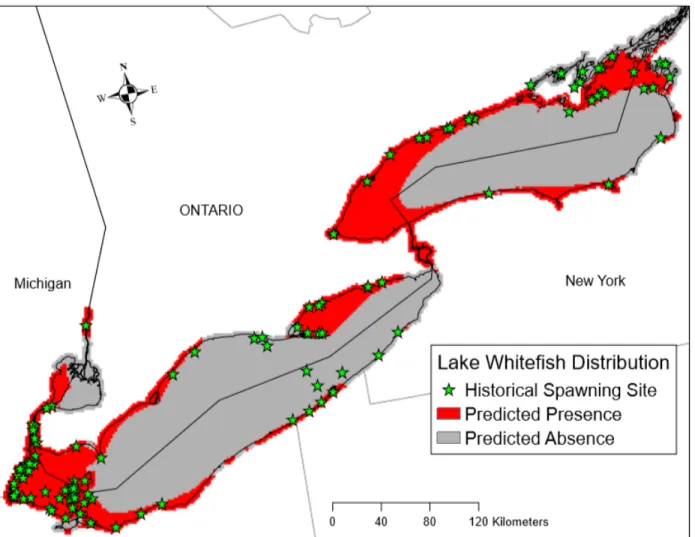
connecting channels restricted to depths less than 25m...31 Figure 3: CART model for Lake Whitefish showing fetch distance and ice cover duration are important variables to be included in the model...32 Figure 4: Output map from Lake Whitefish CART model highlighting predicted areas of
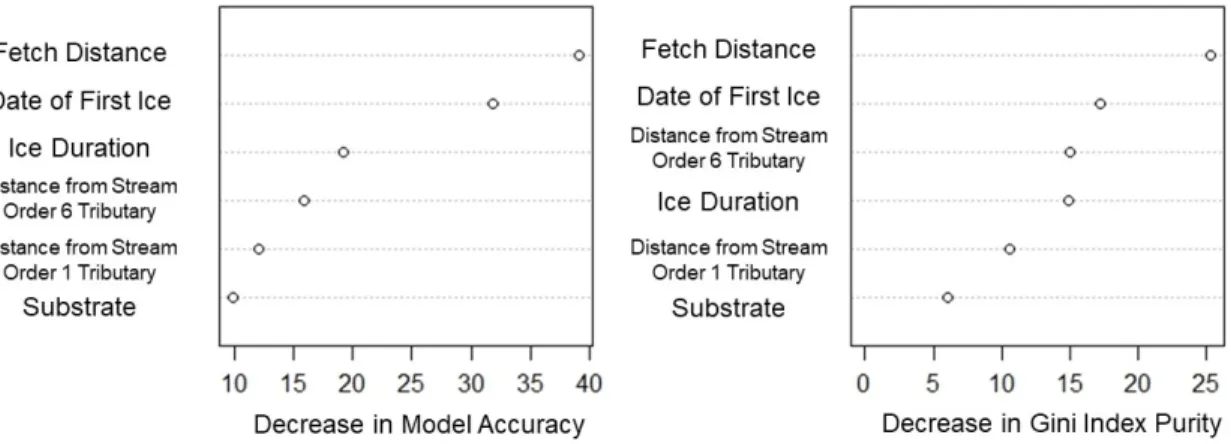
spawning presence and absence across the study area...33 Figure 5: Importance of model variables for the Lake Whitefish random forest model ranked according to overall model accuracy when that variable is removed (left) and decrease in purity of the node when that variable is not considered in the division (right)...34 Figure 6: Interaction plot from the Lake Whitefish random forest model showing highest
probability for spawning presence occurs in regions where fetch distance is lower than
approximately 30km and the date of first ice is between December 25and January 3...35 Figure 7: Output map from Lake Whitefish random forest model highlighting predicted areas of spawning presence and absence across the study area...36 Figure 8: CART model for Cisco showing ice duration, fetch distance, substrate, and date of first ice are important variables to be included in the model...37 Figure 9: Output map from Cisco CART model highlighting predicted areas of spawning
vi
Figure 10: Importance of model variables for the Cisco random forest model ranked according to overall model accuracy when that variable is removed (left) and decrease in purity of the node when that variable is not considered in the division (right)...39 Figure 11: Interaction plot from the Cisco random forest model showing highest probability for spawning presence occurs in regions where ice cover duration is between 55 and 65 days...40 Figure 12: Output map from Cisco random forest model highlighting predicted areas of
spawning presence and absence across the study area...41 Figure 13: Overlapping results from Lake Whitefish and Cisco CART models...42 Figure 14: Overlapping results from Lake Whitefish and Cisco random forest models...43
vii
Table of Contents
Abstract...ii Acknowledgments...iii List of Tables...iv List of Figures...v Introduction...1 Methods...7 Results...12 Discussion...18Tables and Figures...25
1
Introduction
Many forms of coregonines historically occurred throughout the Great Lakes basin
(Koelz 1927; Loftus 1980). In Lake Erie and its connecting channels, Cisco Coregonus artedi are believed to be nearly extirpated, and Lake Whitefish Coregonus clupeaformis, while in recovery since the 1960s (Baldwin et al. 2006), have been observed in reduced numbers since the late 20th century (Roseman et al. 2007). Similarly, numbers of Cisco and Lake Whitefish have declined from historic levels in Lake Ontario, although populations in eastern Lake Ontario are believed to be recovering (McKenna and Johnson 2008). These species were important during the 1800s and early 1900s when fisheries harvested them heavily (Rathbun and Wakeham 1897; Van Oosten 1930). In Lake Erie, 19,000,000 pounds of Cisco were reportedly taken in 1885, with 8,000,000 pounds caught by fishermen from Sandusky alone (Smith and Snell 1890). Both Cisco and Lake Whitefish played important roles as prey species to piscivorous fish like Lake Trout
Salvelinus namaycush, in some cases competing against non-native species like Rainbow Smelt
Osmerus mordax (Stockwell et al. 2009; Zuccarino-Crowe et al. 2016). Restoring populations could allow these native species to reenter and restore the food web (Schmidt et al. 2011) and lead to an increase in catch by fisheries as well.
Low numbers of Lake Whitefish and Cisco in the lower lakes have led to discussions centered around re-introduction and supplemental stocking to help populations recover (Oldenburg et al. 2007). An important step for reintroduction or supplemental stocking of a species is to find suitable regions to stock (Edsall and Kennedy 1995; Bolland et al. 2010). Problems may arise if unsuitable habitats are selected as sites for developing a new population, including loss of larval stock by predation, inadequate habitat for spawning, or a significant loss of individuals from competition (Jude et al. 1981; Zimmerman and Krueger 2009). Hence, a
2
major component of species reintroduction or restoration involves restoration of habitat, often for adequate spawning habitat (Lewis et al. 1996; Kondolf 2000; McLean et al. 2015). Researchers and managers have found that by restoring spawning habitat and developing substrates and reefs that replicate natural habitats, some reintroduced species have had subsequent successful
spawning (Palm et al. 2007; Marsden et al. 2016; Leblanc et al. 2017).
Spawning habitats are commonly revisited by iteroparous fish, depending on the species and its life cycle, with some species even showing spawning site fidelity (Forsythe et al. 2012; Hayden et al. 2018). Identifying key habitat locations historically used for spawning is one method for selecting good sites for restoration or species reintroduction. This approach is particularly useful for species like Lake Whitefish and Cisco whose numbers have been drastically reduced over the last century (Berst and Spangler 1972; Eshenroder et al. 2016). Finding habitat locations across the Great Lakes using these historically relevant sites requires a set of preference parameters from important environmental factors related to coregonine
spawning.
Because spawning of Lake Whitefish and Cisco occurs in the fall (Organ et al. 1978; Goodyear et al. 1982), ice is one factor that may play a role in the early life history of Lake Whitefish and Cisco. Ice cover protects incubating eggs from exposure to wind and wave action during winter, thus areas that are more exposed to the elements have a higher egg mortality (Taylor et al. 1987; Freeberg et al. 1990). Ice concentration, cover, and thickness are all factors that vary across the Great Lakes throughout the years (Assel et al. 2003; Mason et al. 2016). Water depth is one factor that affects ice concentration, which is the percentage of an area that is covered by ice, and areas with shallow water will generally reach higher levels of ice
3
morphometry of Lake Erie and Lake Ontario result in different ice patterns (Wang et al. 2012), evaluating the duration of ice concentration above a low threshold that is consistently found in both lakes could allow for more accurate results in a lake-wide ice data analysis. Therefore, the duration of ice cover of at least 10% ice concentration across an 1800m by 1800m grid in the study area was included. The date of first ice, or the day when ice concentration reached 50%, was also included in this study to measure consistency of ice presence in these same gridded areas. In an evaluation of ice concentration and its influence on predicting Lake Whitefish recruitment, 40% and 70% ice concentration were most significant for areas with more open water and less open water, respectively (Brown et al. 1993). Because my study occurred across two morphologically different lake basins, 50% ice concentration was used when calculating the date of first ice across the study area.
Fetch, or the measurement of uninterrupted distance that wind travels across a body of water, is often used to quantify the influence wind can have on aquatic habitat (Rohweder et al. 2012). It can be included in habitat models to covey levels of wave energy put into a system by wind action (Burton et al. 2004; Schall et al. 2017). Wind can affect aquatic habitats through soil erosion or water circulation, and can influence parameters such as water clarity and dissolved oxygen (Olson and Ventura 2012). Wind has also been shown to affect egg viability for many different fish species. For example, an increase in fetch distance was correlated with decreased egg survival of Lake Trout (Fitzsimons 1995). Wind currents can also benefit egg incubation by removing fine sediments where eggs were deposited (Sly 1988; Gunn 1995). Areas with low to intermediate fetch distances within the lakes may provide habitats with less disturbance by wind and wave energy and could be preferred spawning locations for coregonines (Sly and Schneider 1984; Marsden et al. 1995).
4
Currents produced by tributaries could have similar effects to wind currents since both have the energy to move fine sediments within habitats, including reefs. Reefs located further from stream outlets could be more likely to have particles settled into the interstitial spaces where Lake Whitefish tend to deposit eggs, making them less desirable spawning locations. Too much current velocity, potentially produced by a tributary with higher stream order, may lower egg viability through egg burial and physical disturbance (Manny et al. 1995). Streams can also be beneficial to lake systems by acting as sources of dissolved oxygen (O’Connor 1967), because dissolved oxygen concentration is a common measurement for habitat quality (Batiuk et al. 2009; Missaghi et al. 2017). The distance from stream outlet points to a potential spawning site could reflect a preference for areas with increased dissolved oxygen concentrations. Including both low and high stream order as variables in the study could also indicate selection for higher or lower current velocities.
Substrate use is flexible for both Lake Whitefish and Cisco, although spawning in rock, reefs, stone crevices, sand, and gravel substrates is typically observed (Berst and Spangler 1972; Goodyear et al. 1982; Lane et al. 1996). Larger substrate sizes like cobble and gravel benefit broadcast spawners like coregonids by providing protected and oxygenated sites for eggs during incubation (Gunn 1995). While these substrates were important for these species historically, increased anthropogenic activity along the shorelines of the Great Lakes has been damaging to substrate quality and composition nearshore (Goforth and Carman 2005). In areas where preferred spawning substrate may have been degraded over time, construction of artificial reefs can be considered. Some artificial reefs attempt to replicate quality substrate used by target fish for spawning (McLean et al. 2015).
5
Water depth is often an important factor considered for fish spawning habitat. For Lake Whitefish and Cisco, spawning has usually been observed at depths no more than 25 meters (Goodyear et al. 1982). Because Lake Whitefish and Cisco are primarily recognized as spawning nearshore and in tributaries, spawning presence will be correlated with depth. This suggests that incorporation of depth as a factor in a suitability model will likely have a masking effect on other included factors. Excluding depth from a habitat suitability model would result in a more
thorough investigation into additional characteristics, but depth is recognized as an important consideration for future habitat restoration projects. In this study, depth was incorporated by restricting the presence and absence points used to those found at depths less than 25 meters.
Suitability models can be created using habitat characteristics of a study area, along with species presence and absence data, to predict additional locations where that species would be present. Classification and Regression Tree (CART) modeling is one method frequently used for species distribution modeling (Franklin 2009). The CART model relies on binary splits at each node of a decision tree (DT) where points are placed in subcategories through yes/no questions answered at each node (Muñoz and Felicísimo 2004). For a given parameter in the DT, a statement for a specific data attribute is paired with a range of values associated with that attribute. Many studies have used CART to predict where species might occur or where suitable habitat might be present according to factors included in the model (Moisen et al. 2006; He et al. 2010). Applying these predictions to maps of a study area can then reveal locations of focus for future management.
The CART method is also capable of using historical data to model current distributions and make comparisons to present or projected environmental conditions. For data sets using historical or museum accounts of presence locations, one strategy for developing absence points
6
involves using a random point generator in a GIS (Muñoz and Felicísimo 2004). An equal number of absence and presence points is required for accurate results. Thus, in studies where only presence points are available or only a few absence points have been recorded, pseudo-absence points can be generated without using a dataset of false positives (Mainella 2016). Other species distribution models, including maximum entropy (MaxEnt) models, do not require the use of absence points (Elith et al. 2011), which is another alternative for studies where only presence data is available. The MaxEnt model can be a more difficult approach in studies when multiple functional forms are used to interpret the effects of the environmental variables
included, making the final interpretation of the model unclear (Syfert et al. 2013). Habitat
suitability indexes are also used for identifying suitable areas for species, but these methods have been criticized for their lack of reliability (Roloff and Kernohan 1999). Due to the user-friendly interpretations, applicability to mapping formats, and mutual exclusivity methodology of DT models (Olden and Jackson 2002), the CART model was selected for this study.
One major downfall of CART modeling is its lack of stability (Franklin 2009). Decision trees created using the CART method can have significantly different results by removing or adding single factors, which lower reliability. One model that addresses this issue is the random forest model. Random forest models work in the same way as classification and regression trees by using binary splits, but instead of producing a single tree, hundreds of trees are produced and averaged for an output result. Random forest outputs can be viewed as mapped distributions, which can be informative for predictive modeling. Because random forest models have higher stability than single CART models, I also used the random forest model to verify CART results.
In this study I predicted suitable spawning habitat for Lake Whitefish and Cisco in the lower lakes and their connecting channels using the CART and random forest models. I
7
identified areas in Lake Erie and Lake Ontario, as well as Lake St. Clair, the St. Clair River, the Detroit River, the Niagara River, and the St. Lawrence River, where spawning habitat should be available based on selected characteristics which, in turn, could be areas where future restoration or stocking efforts could be invested.
Methods
Historical data points for spawning sites were obtained from the Goodyear Spawning Atlas on the GLAHF webpage (Wang et al. 2015). Due to some inaccuracies in point location, a more thorough investigation into the Spawning Atlas (Goodyear et al. 1982) was conducted. Sources within the Spawning Atlas were reviewed for specific spawning locations, and locations described as being used for non-spawning purposes or as nursery areas were removed. Points previously located outside of the lake boundary were investigated and moved accordingly into the study area. Data sets included 112 presence points for locations of historical spawning of Lake Whitefish (Fig. 1) and 53 presence points for Cisco (Fig. 2) across the entire study area, which includes Lake Erie, Lake Ontario, and connecting channels. Presence and absence points were restricted to depths less than 25m. Absence data points were created using the “Generate Random Points” function in ArcGIS 10.5. The number of absence points generated was equal to the number of presence points across the study area, which gave a total of 224 data points for Lake Whitefish and 106 points for Cisco. To decrease potential point location bias, equal numbers of absence and presence points were generated separately in Lake Erie and Lake Ontario regions for each species. The Lake Erie region (including Lake St. Clair, the Detroit River, and the St. Clair River) contained 78 presence points for Lake Whitefish along with 29 presence points for Cisco. The Lake Ontario region (including the Niagara River and the lower
8
region of the St. Lawrence River) contained 34 presence points for Lake Whitefish and 24 presence points for Cisco.
The role of ice cover was incorporated into the model through ice cover duration and the date of ice onset. Ice cover duration and ice onset dates were obtained from GLAHF (Wang et al. 2015). Annual duration data for ice years 1973- 2017 were extracted and averaged. The cell statistics tool in ArcGIS 10.5 was used to average the layers by cell across the 45-year period to represent the number of days that ice was present at each cell for an average year. Ice onset date was catalogued using numerical values by assigning December 1 as day “101” in the data set. Consecutive days were numbered in order after 101 so each point had a number value
representing day of the year. Ice onset date was considered when cells had an ice concentration of at least 50%, and cells that never reached 50% ice cover for a given year were assigned an ice onset date of “NoData” for that year. All cells reached 50% ice cover at some point during the 45-year period. No presence or absence points occurred over a “NoData” site. Data layers for ice onset were also averaged across the 45-year period to create one layer using the cell statistics tool. Each cell size in both the ice cover duration and the ice onset date grids measured 1800m by 1800m.
A data layer for fetch, which represents the uninterrupted and unobstructed distance wind can travel across a body of water, was created to explore whether exposure to wind influenced spawning habitat selection. Fetch data was obtained from Mason et al. (2018) who calculated effective fetch distance using directional fetch rasters multiplied by the percent frequency that wind blows in each measured direction from buoy data from 2010 and 2014. Fetch data across Lake St. Clair, Lake Erie, and Lake Ontario for years 2010 and 2014 were averaged together for each cell. Because the fetch layer had cell sizes of 30m by 30m, the layer was resampled in
9
ArcGIS 10.5 using bilinear interpolation, which finds new cell values using bilinear interpolation and weighted distance averaging of the four nearest cells. After resampling, the fetch layer had cell sizes of 1800m by 1800m to match both ice data layers.
The distance from tributary outlets was calculated to determine the importance of
proximity to areas of potential substrate disruption and added dissolved oxygen. Tributary outlet data was obtained from GLAHF, which identified the locations of streams with Strahler stream orders of 1-7 (Wang et al. 2015). Lower order streams are characteristically smaller in size with a low flow rate, while higher order streams are located further downstream, are larger in size, and have a higher flow (Leopold and Maddock 1953; Frissell et al. 1986). All connecting channel sites, which include the St. Clair River, Detroit River, Niagara River, and St. Lawrence River were evaluated as locations within a high order stream and were given a distance of 0km from a high order stream. Watershed outlet points were selected to be within 0.5km of the study area shoreline. Stream outlet points were selected and exported according to Strahler stream order. Two layers were developed to represent distance from a low stream order (Strahler stream order 1) and a high stream order (Strahler stream order 6). The Euclidean distance tool was applied across the study area for both stream orders to create two raster layers with cell sizes of 1800m by 1800m.
Substrate was included in the model to predict the presence of spawning over mud, sand, hard, or clay substrate - the four categories (not including “unknown”) listed in the substrate raster layer downloaded from GLAHF (Wang et al. 2015) with cell sizes of 30m by 30m. In ArcMap 10.5, the substrate layer was resampled using the “majority” technique, which creates new cell values by considering values of surrounding cells and assuming the majority value. The output raster layer had cell sizes of 1800m by 1800m.
10
Inverse distance weighting interpolation was applied to substrate, ice cover duration, ice onset date, and fetch distance data layers to create consistency across layers. This technique assigns data values to areas with otherwise unknown data using known surrounding values, where values closer to the unknown cell carry a higher weight in the calculation (Lu and Wong 2008). These interpolated raster layers filled in data gaps within the study area, where most unknown data values were located within the St. Clair River, Detroit River, Niagara River, and St. Lawrence River. Cells were filled to extend just outside the shoreline to provide data values to presence and absence points close to the shoreline. To do this, a 3km buffer was created around the shoreline polygon containing Lake Erie, Lake Ontario, and connecting channel boundaries. The “Extract Values to Points” tool was used to assign values from each of the raster data layers to the point layers for Cisco and Lake Whitefish spawning sites.
The “rpart” package in RStudio was used to create the CART models for Cisco and Lake Whitefish. For each species, training sets were created using 80% of the data and were used to create the decision trees. Test sets were created from the remaining 20% of the data and were applied to the decision trees created by the training data to test the accuracy of each model. Because of the relatively low sample size in Lake Ontario, the data for the entire study area of Lake Erie, Lake Ontario, and the connecting channels were pooled together to create one model for each species as opposed to individual lake models. This method was also applied to the random forest models (two models spanning the entire study area). The training dataset for Lake Whitefish contained 180 points and the test data set contained 44 points. The training dataset for Cisco contained 86 points and the test data set contained 20 points. For the Lake Whitefish CART model, the minimum split value was equal to 10, meaning that at least 10 observations must be met to create a split in the tree. The minimum number of points required to create a
11
terminal node was set to 10, and 10 cross validations were completed. The maximum node depth for the final tree was also equal to 10. These restriction values were chosen to create
homogenous groups while refraining from overfitting the data (De’ath and Fabricius 2000). For the Cisco CART model, minimum split value and minimum number of points for a terminal node were set to 5. The minimum split values for the Cisco model were lower than those of the Lake Whitefish model because of the difference in available data points.
CART model decision trees were interpreted by following branches and splitting parameters to each terminal node. Data that have similar values for that attribute are grouped together by answering the yes/no questions such that if the answer to the statement is “yes” then the statement is true for the group at the node and when the statement is answered “no” then the statement is false. Parameter statements that were “true” were followed down the left side, and statements that were “false” were followed down the right side. Each box represents a node of the tree where points sharing common values were grouped together (Figure 3; Figure 7).
The “randomForest” package in R Studio was used to create predicted spawning location maps by summarizing 1000 classification trees for each species. This model was also used to rank the variables by level of importance to show which factors are potentially most important in predicting spawning presence. The same factors used in the CART model were included in the random forest model. The same training and test datasets for each species were used as well. Variable importance was first measured according to percent decrease of overall model accuracy when a variable is omitted from the model. Importance was also measured by the average
decrease in Gini impurity value due to variable omission. The Gini index measures purity of the node, where higher node purity means lower variance within the node and increased variability across nodes. This value is measured across all trees at branching splits using that variable and
12
averaged together. Each model was evaluated with an estimated error rate and confusion matrix to measure misclassification by the model. Model performance was also evaluated using the area under the curve statistic (AUC) for both training and test data, where an AUC value of 0.5 means the model is uninformative and predicts at the same rate as a chance estimate.
Results
Variable Summary
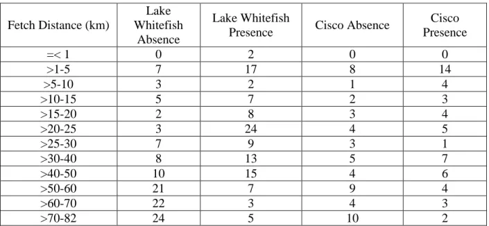
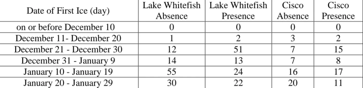
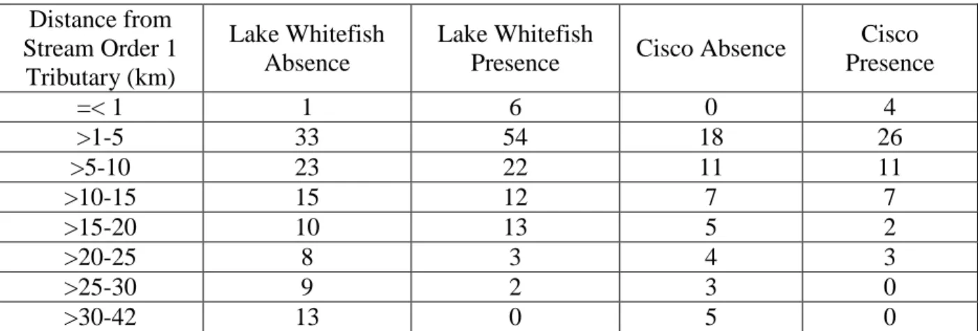
About 60% of Lake Whitefish absence points occurred in areas where fetch distance was greater than 50km, while 54% of presence points occurred in areas with a fetch distance equal to or less than 25km (Table 1). Frequencies of Cisco absence points varied across fetch distances, while 26% of presence points occurred in areas where fetch distance was between 1km and 5km (Table 1). The highest frequency of Lake Whitefish absence points occurred in the ice duration range of 51 to 60 days, while the highest frequency for presence points collectively occurred between 61 and 80 days (Table 2). The highest frequency of Cisco presence points fell in the ice duration range of 61-70 days, while the highest frequency of Cisco absence points occurred between 51 and 60 days for ice duration (Table 2). The highest frequency of Lake Whitefish absence sites occurred with first ice dates from January 10 to January 19 (Table 3). The highest frequency of Lake Whitefish presence sites occurred with first ice dates from December 21 to December 30 (Table 3). The highest frequencies of Cisco absence points occurred between first ice dates of January 20 and January 29 while most Cisco presence points occurred between January 10 to January 19 (Table 3). Both Lake Whitefish presence and absence sites and Cisco presence and absence sites had the highest frequencies of values for distance from a stream order 1 tributary falling within the range of 0km to 10km, but the frequencies of presence sites at this
13
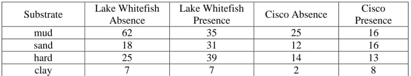
distance were nearly double the frequencies of absence sites (Table 4). The highest frequency of Lake Whitefish absence points for distance from a stream order 6 tributary fell in the range of 80km and 120km, while presence points had the highest frequency in the range of 40km to 60km (Table 5). Both 68% of Cisco absence points and 68% of presence points had a distance from a stream order 6 tributary that was less than 60km (Table 5). The highest frequencies of Lake Whitefish and Cisco absence points occurred over mud substrate, while presence points for both species occurred with similar frequencies over mud, sand, and hard substrates. Frequencies for both Lake Whitefish and Cisco presence points were much lower over clay substrate (Table 6).
Lake Whitefish CART
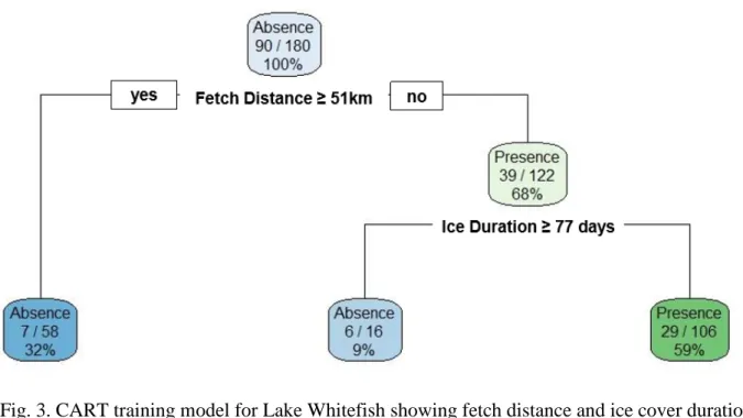
Using the training dataset (N=180), the Lake Whitefish CART model predicted 106 sites (59%) with spawning presence and 74 sites (41%) with spawning absence (Fig. 3; Table 7). Using the test dataset (N=44), the model successfully predicted whether Lake Whitefish spawned (or did not spawn) at a given site with 77% accuracy. Fetch distance was the primary splitting factor, and areas with a fetch distance greater than or equal to 51km were predicted to be non-spawning sites, with an 88% accuracy rate. Areas with fetch distances less than 51km were predicted to be spawning sites with 68% accuracy. Accuracy rate for predicting spawning sites was even higher (i.e., 73%) for sites with a fetch distance less than 51km and ice cover duration less than 77 days. Conversely, areas with a fetch distance less than 51km and ice cover duration greater than or equal to 77 days were predicted to be non-spawning sites with a 63% accuracy rate. The output from the CART model was used to produce a map (Fig. 4) highlighting areas of predicted spawning presence in the study area. Major sites of predicted spawning presence included the western region of Lake St. Clair, the Detroit River, the western basin of Lake Erie,
14
and the western region of the eastern basin of Lake Erie. In Lake Ontario, predicted areas of presence include the western region, the southern shoreline, and the northeastern region, as well as the Niagara River.
Lake Whitefish random forest
The random forest model for Lake Whitefish classified spawning sites with 77% accuracy and non-spawning sites with 67% accuracy (Table 8). The prediction error for the model was estimated at 28%. Variables were ranked by importance according to overall decrease in model accuracy and Gini index purity (Fig. 5). For overall model accuracy, fetch was most important followed by date of first ice, ice duration, distance from tributary stream order 6, distance from tributary stream order 1, and substrate. When ranked according to decrease in Gini index purity, the most important variable was also fetch, followed by date of first ice, distance from tributary stream order 6, ice duration, distance from tributary stream order 1, and substrate (Fig. 5). Specific parameters were not extracted from the random forest model because this would involve extracting a single tree from the 1000 trees used to build the model, which would not accurately reflect model results. Instead, standard evaluation of the random forest model involves overall ranking of variable importance using all trees that were built (James et al. 2013). The AUC value calculated for training data was 0.8144 and for test data was 0.8037, indicating a much higher prediction success rate than random values.
An interaction plot was developed to compare fetch, the primary variable of importance, to the second most important variable, date of ice onset. Spawning presence was predicted with over 75% probability in areas where fetch distance was below approximately 30km and date of ice onset was between December 25 and January 3 (Fig. 6). The outputs from the 1000
15
classification trees of the random forest were combined to produce a map (Fig. 7) highlighting areas of predicted spawning presence and predicted spawning absence in the study area. The western basin of Lake Erie was a major area of predicted Lake Whitefish spawning presence, along with the northwestern region of Lake Ontario, northeastern Lake Ontario around Chaumont Bay, and the Bay of Quinte. The Detroit River, parts of the St. Clair River, the western region of Lake St. Clair, and the Niagara River were predicted areas of spawning presence as well, along with the western basin of Lake Erie and the Bass Island region. When comparing spawning presence predictions from the CART model and the random forest model for Lake Whitefish, 83% of the random forest predicted area overlapped with the CART predicted area, while 63% of the CART area overlapped with the random forest area. For spawning absence predictions, 85% of the random forest predicted area overlapped with the CART predicted area, while 94% of the CART area overlapped with the random forest area.
Cisco CART
Using the training dataset (N=86), the Cisco CART model predicted 42 sites (49%) with spawning presence and 44 sites (51%) with spawning absence (Fig. 8; Table 9). Using the test dataset (N=20), the model predicted whether Cisco spawned (or didn’t spawn) at a given site with 55% accuracy, which is essentially no prediction. The low accuracy rate is likely because of the lower sample size compared to the Lake Whitefish model. Ice cover duration was the primary splitting factor, and areas with an ice cover duration greater than 56 days were predicted to be spawning sites with an accuracy rate of 62%. Areas with an ice cover duration greater than 56 days and a hard or clay substrate were predicted to be spawning sites with an accuracy rate of 89%. Areas with a substrate of mud or sand and an ice duration greater than 56 days but less than
16
70 days were predicted to be spawning sites with an accuracy rate of 72%. Accuracy for predicting spawning sites was highest (100%) for sites with an ice cover duration between 56 and 70 days, a mud or sand substrate, and a date of first ice on or before January 13.
Additionally, areas with an ice cover duration less than 56 days and a fetch distance less than 45km were predicted to be spawning sites with a 64% accuracy rate. The output from the CART model was used to produce a map (Fig. 9) highlighting areas of predicted spawning presence in the study area. Major sites of predicted spawning presence included areas within the western basin of Lake Erie, the western region of the eastern basin of Lake Erie, and most of the Lake Erie shoreline. In Lake Ontario, spawning presence was predicted in Sodus Bay, Irondequoit Bay, Chaumont Bay, sections of the lower St. Lawrence River, and the western region of the lake.
Cisco random forest
The random forest model for Cisco classified spawning sites with 63% accuracy and non-spawning sites with 63% (Table 10). The prediction error for the model was estimated at 37%. For overall model accuracy, ice duration was the most important variable followed closely by fetch distance (Fig. 10). Substrate, distance from tributary stream order 1, date of first ice, and distance from tributary stream order 6 followed in importance. When ranked according to decrease in Gini index purity, ice duration was the most important variable, followed by fetch distance, distance of tributary stream order 1, distance from stream order 6, date of first ice, and substrate (Fig. 10). Model performance was evaluated using the area under the curve statistic (AUC) for both training and test data. The AUC value calculated for training data was 0.7350 and for test data was 0.8200.
17
Although specific values of the random tree model could not be produced overall, an interaction plot was developed to quantitatively compare ice duration, the primary variable of importance, to the second most important variable, fetch distance. Spawning presence was predicted with 75% probability or higher in areas where ice duration was between 55 and 65 days (Fig. 11). Spawning presence was predicted with 25% probability or lower when fetch distance was greater than 50km and ice duration was less than 55 days (Fig. 11). The outputs from the 1000 classification trees of the random forest were combined to produce a map (Fig. 12) highlighting areas of predicted spawning presence in the study area. Major sites of predicted spawning presence included the Detroit River, the shoreline of Lake St. Clair, the lower St. Lawrence River, the western region of the Bay of Quinte, and the Chaumont and Henderson Bay areas of Lake Ontario. Almost all of the Lake Erie shoreline was predicted for spawning
presence as well, especially in the central basin. Spawning absence was predicted across most of the southern shore of Lake Ontario except for small regions near Irondequoit Bay and Sodus Bay. When comparing spawning presence predictions from the CART model and the random forest model for Cisco, 70% of the random forest predicted area overlapped with the CART predicted area, while 61% of the CART area overlapped with the random forest area. For spawning absence predictions, 86% of the random forest predicted area overlapped with the CART predicted area, while 90% of the CART area overlapped with the random forest area
CART overlap for Lake Whitefish and Cisco
Predicted presence and absence sites for Lake Whitefish and Cisco were combined to reveal areas of overlap (Fig. 13). Presence areas included the southern Lake Erie shoreline in the central
18
basin, the Bass Island region, the lower Detroit River into the western basin, the western area of Lake Ontario, Sodus Bay, Irondequoit Bay, and the northern region of Lake Ontario.
Random forest overlap for Lake Whitefish and Cisco
Predicted presence and absence sites for Lake Whitefish and Cisco were combined to reveal areas of overlap (Fig. 14). Presence areas included the southern Lake Erie shoreline, the Bass Island region, the Detroit River, the St. Clair River, the Bay of Quinte, and the lower St. Lawrence River.
Discussion
CART and random forest models were used to predict spawning sites for coregonines in the lower lakes and connecting channels. In the CART model for Lake Whitefish, fetch distance and ice cover duration were significant variables predicting spawning sites. This model predicted spawning sites with 77% accuracy when applied to a test dataset. In the random forest model for Lake Whitefish, significant variables were fetch distance and date of first ice, which predicted spawning sites with an accuracy rate of 77% and non-spawning sites with an accuracy rate of 67%. In the CART model for Cisco, ice duration, fetch distance, substrate, and date of first ice were significant variables for predicting spawning sites. This model predicted spawning sites with only 55% accuracy when applied to a test data set. In the random forest model for Cisco, ice duration and fetch distance were significant variables for predicting spawning sites with an accuracy rate of 63% and for non-spawning sites with an accuracy rate of 63%. Collectively, the predictive variables from this study highlight important areas for Lake Whitefish and Cisco
19
spawning and also draw attention to parameters that are influential for predicting spawning habitat.
Fetch distance < 51km was the most important variable in both the CART and random forest models for predicting spawning sites for Lake Whitefish. Fetch distance < 45km was an important predictor factor for Cisco in the CART and random forest models as well. The
underlying mechanisms for a relatively short fetch distance were reduced risk of incubating eggs being disrupted by wind or wave energy (i.e., more protected habitat) and the facilitation of earlier ice formation. For example, Manny et al. (1995) found that Lake Trout eggs located in Partridge Island Reef, which had a 90% higher mean wave energy than the second study area at Port Austin Reef the week after deployment, had a higher percentage of egg mortality. In my study, since both spawning and non-spawning sites were restricted to depths less than 25m, nearshore sites could not have been selected simply because of a shallower depth. Both the CART models and random forest interaction plots predict higher probabilities of spawning in areas where fetch distance is less than 51km for Lake Whitefish and less than 45km for Cisco, which is supported by the higher frequencies of non-spawning sites falling in ranges of fetch distances greater than 50km. Looking at smaller lakes in comparison, Nohner and Diana (2015) focused on fetch within lakes of Wisconsin with surfaces areas ranging from 0.5km2 to 14.52km2 and found that Muskellunge Esox masquinongy were predicted to select for spawning habitat with sheltered fetch (36-56m) and select against habitats with large effective fetches. In a study on Lake Trout spawning habitat selection in smaller-sized lakes, Flavelle et al. (2002) found that fetch played an important role as well, although their study resulted in smaller values and a narrower range (0.8-2.3km) compared to my study. Although my predicted values for fetch distance are much higher than similar modeling studies measuring fetch, the basin-wide scale for
20
both models used fetch distance to initially highlight areas that would have a lower fetch distance relative to the basin, including the Bass Island region of the Lake Erie western basin, connecting channels, shorelines, and smaller bays– this information was a necessary foundation for
additional variables to build upon to further specify predicted spawning sites.
Along with fetch distances, either duration of ice cover or date of first ice predicted spawning sites for both species. In the CART model, ice cover duration was an important
variable for Lake Whitefish, whereas the random forest model showed the date of ice onset as an important variable. For Cisco, ice cover duration was an important variable for both the CART model and the random forest model, and date of first ice was an important variable in the CART model. These results aligned with the hypothesis that ice cover would play a role in spawning presence for both species. According to the random forest interaction plot for Lake Whitefish, the highest probability of spawning would occur when the date of first ice is between December 25 and January 3, which is relatively early in winter. Lynch et al. (2015) similarly found that ice cover in December significantly influenced modeled Lake Whitefish recruitment at two of the shallower management areas in Lake Superior in a study focusing on 13 management locations within the 1836 Treaty Waters of lakes Superior, Huron, and Michigan. In Lake Erie, Lawler (1965) found that stronger year classes of Lake Whitefish were associated with years where water temperatures dropped to ideal spawning temperatures (6.1°C) early in the fall and longer incubation periods occurred. Although my study also predicted spawning presence for Lake Whitefish in areas with an ice duration less than 77 days, the significance of an early ice onset date is consistent with the findings of Lynch et al. (2015) and Lawler (1965). Only 9 of the 112 Lake Whitefish presence sites had an ice cover duration over 77 days. Spring weather conditions have also been found to play a role in recruitment (Freeberg et al. 1990) which my study did not
21
consider beyond ice cover duration. For Cisco, spawning presence was predicted by the CART model in areas where ice cover was over 56 days. These results are more consistent with findings from Lake Whitefish recruitment studies in Lake Michigan, where the number of days of 40% ice concentration coverage was the most important variable in Northern Green Bay (Brown et al. 1993). Similarly, in Grand Traverse Bay, eggs consistently protected by ice cover during a 122-day incubation period had the highest viability (Freeberg et al. 1990). An ice duration of 56 to 70 days was also specified for predicting spawning presence in the Cisco CART model when the date of first ice is on or before January 13. Of the 53 Cisco presence sites, there were 17 (32%) that had an ice duration over 70 days (Table 2). While my study shows that ice cover plays an important role in spawning habitat for Lake Whitefish and Cisco, considering spring weather conditions may also be important for sites to have successful recruitment.
Substrate type appeared as an important factor for Cisco spawning sites in the CART model. Because substrate ranked lowest according to Decrease in Gini Index Purity in the random forest model, this means that with the substrate variable there is a higher likelihood of misclassification when the nodes created from splits by the substrate variable are used to randomly classify dataset points (Breiman et al. 1984; Cutler et al. 2007). However, the relatively high ranking in overall model accuracy suggests it is still important to include in the model. In the Cisco CART model, spawning presence was predicted for all 4 substrate types under specified conditions. In areas where ice duration was over 56 days and substrate was hard or clay, the highest percentage of spawning sites were predicted to occur. However, spawning presence was still predicted over sand or mud substrate when ice duration was between 56 and 70 days and the date of first ice was on or before January 13. Historically, substrate preference has been noted as flexible for both Cisco and Lake Whitefish, although many sources note the
22
use of rock, reefs, stone crevices, sand, and gravel substrate during spawning (Rathbun and Wakeham 1896; Goodyear et al. 1982). More recent studies suggest that regions of the Great Lakes influenced by paleo-ice streams (fast-flowing streams within ice sheets from glaciation events) may also be predictors for Lake Whitefish and Cisco spawning habitat, specifically regarding substrate (Riley et al. 2017). These ice streams transported ice and sediment, and those within the Laurentide Ice Sheet can be linked to sedimentation and erosion patterns within the Great Lakes (Paterson 1994; Bennett 2003). This would allow for further spawning habitat predictions using substrate as a factor since the locations of these paleo-ice streams can be mapped as well (Krabbendam et al. 2016). Although substrate was an important variable to include in the CART and random forest models, my study showed there was no real significant substrate type used to predict spawning presence.
Both models for Lake Whitefish and Cisco did not include distances from tributaries as important variables. These variables were considered because of the influence that high stream flow or wave action can have for spawning substrate and developing eggs, including
sedimentation, dislodgment, and physical disturbance (Eschendroder et al. 1995). I hypothesized that areas affected by habitat disruption due to proximity to a high stream order tributary may be avoided by species like Lake Whitefish and Cisco. However, the connecting channels can be classified as areas of high wave energy compared to the basin habitat and spawning for both Lake Whitefish and Cisco has been observed historically in connecting channels (Goodyear et al. 1982). My study predicted spawning sites for both species in both models to some extent in these connecting channels without a significant input from the high order tributary variable. While the distances from a high stream order tributary and a low stream order tributary were not important
23
variables in any of my models, a more localized study measuring wave energy from tributaries could be informative in a smaller-scale habitat study.
While biases can often be introduced in predictive modeling, this study aimed to lower variable biases as much as possible. Ice cover data can be highly variable from year to year due to a combination of short-term and long-term factors (Wang et al. 2012). By averaging data across all available ice years (more than 40 years), this study aimed to include a range of possible weather years to reduce any bias associated with ice cover. Fetch distance averaged from
previous data (Mason et al. 2018) was also averaged across two different study years, which summarized the only available years when Lake St. Clair, Lake Erie, and Lake Ontario data coincided. Resampling of the data to larger pixel sizes (30x30m to 1800x1800m) allowed the data to remain true to these original calculations, although some bias may have been introduced through the resampling process when compared to a new calculation set to the 1800x1800m scale. The higher accuracy rate for the Cisco random forest model compared to the Cisco CART model is likely because the random forest model used 1000 classification trees to produce the best model. Both Cisco models resulted in a lower accuracy rate compared to the Lake Whitefish models, and this is likely due to the difference in sample sizes.
The basin-wide focus of this study allowed variables to be predictors at a larger scale instead of predicting more localized habitat sites. By highlighting areas where both species are predicted to have spawning sites (Fig. 13; Fig. 14), resources for restoration projects can be focused on areas that both species would theoretically utilize. This is especially useful for areas located within current habitat refuges that were predicted presence sites in these models. While creating lake-specific predictor models was considered, ultimately the entire study area was used as the input for Lake Whitefish and Cisco models due to the larger combined sample size. This
24
study highlights broad locations where local habitat suitability projects could be pursued to find optimal habitat sites selected by these species (Schaefer et al. In review). Because of this, focusing on areas in the lakes that have not been heavily disturbed might prove to be productive for future restoration initiatives. Areas within the study area of my model highlighted as regions with predicted spawning presence coincide with areas where Lake Whitefish and Cisco have recently been found, including the western basin of Lake Erie, the Detroit and St. Clair rivers, and Chaumont Bay (Roseman et al. 2012; George et al. 2017; Prichard et al. 2017). The presence of spawning by Lake Whitefish and Cisco at locations predicted by this model, as well as the presence of current populations coinciding with these same locations, suggests that several sites historically used by Lake Whitefish and Cisco may still be important today. Restoration of habitat locations for native species throughout the Great Lakes has been a popular objective across the region (Hondorp et al. 2014; Manny et al. 2015). This study reaffirms the importance of many historical spawning sites for both Lake Whitefish and Cisco and also identifies new locations that may be of importance for reintroduction or restoration projects in Lake Erie, Lake Ontario, and their connecting channels.
25
Table 1. Frequency of fetch distance values for Lake Whitefish and Cisco presence and absence sites. Fetch Distance (km) Lake Whitefish Absence Lake Whitefish
Presence Cisco Absence
Cisco Presence =< 1 0 2 0 0 >1-5 7 17 8 14 >5-10 3 2 1 4 >10-15 5 7 2 3 >15-20 2 8 3 4 >20-25 3 24 4 5 >25-30 7 9 3 1 >30-40 8 13 5 7 >40-50 10 15 4 6 >50-60 21 7 9 4 >60-70 22 3 4 3 >70-82 24 5 10 2
26
Table 2. Frequency of ice duration values for Lake Whitefish and Cisco presence and absence sites. Ice Duration (days) Lake Whitefish Absence Lake Whitefish
Presence Cisco Absence
Cisco Presence =< 10 0 0 0 0 11-20 6 7 3 5 21-30 6 6 2 4 31-40 6 3 3 0 41-50 5 3 6 1 51-60 57 18 17 12 61-70 9 30 3 14 71-80 13 37 12 9 81-90 7 2 4 3 91-100 0 2 0 0 101-110 3 4 3 5
Table 3. Frequency of first ice date values for Lake Whitefish and Cisco presence and absence sites.
Date of First Ice (day) Lake Whitefish Absence Lake Whitefish Presence Cisco Absence Cisco Presence on or before December 10 0 0 0 0 December 11- December 20 1 2 3 2 December 21 - December 30 12 51 7 15 December 31 - January 9 14 13 7 8 January 10 - January 19 55 24 16 17 January 20 - January 29 30 22 20 11
27
Table 4. Frequency of distance from stream order 1 tributary values for Lake Whitefish and Cisco presence and absence sites.
Distance from Stream Order 1 Tributary (km) Lake Whitefish Absence Lake Whitefish
Presence Cisco Absence
Cisco Presence =< 1 1 6 0 4 >1-5 33 54 18 26 >5-10 23 22 11 11 >10-15 15 12 7 7 >15-20 10 13 5 2 >20-25 8 3 4 3 >25-30 9 2 3 0 >30-42 13 0 5 0
Table 5. Frequency of distance from stream order 6 tributary values for Lake Whitefish and Cisco presence and absence sites.
Distance from Stream Order 6 Tributary (km) Lake Whitefish Absence Lake Whitefish
Presence Cisco Absence
Cisco Presence =< 1 0 9 1 3 >1-5 0 4 1 0 >5-10 2 6 2 1 >10-20 9 10 6 8 >20-40 20 16 9 10 >40-60 21 38 17 14 >60-80 10 11 3 3 >80-120 31 17 7 11 >120-140 12 1 2 2 >140-160 7 0 5 1
28
Table 6. Frequency of substrate values for Lake Whitefish and Cisco presence and absence sites.
Substrate Lake Whitefish Absence
Lake Whitefish
Presence Cisco Absence
Cisco Presence mud 62 35 25 16 sand 18 31 12 16 hard 25 39 14 13 clay 7 7 2 8
Table 7. CART training model results for Lake Whitefish spawning predictions with node classifications and misclassification rates.
Terminal Node (from left) Variables Used Predicted Spawning Activity Misclassification Rate Number of Absence Points at Node Number of Presence Points at Node
1 Fetch Distance Absence 12% 51 7
2 Fetch Distance,
Ice Duration Absence 38% 10 6
3 Fetch Distance,
Ice Duration Presence 27% 29 77
Table 8. Classification accuracy for the Lake Whitefish random forest model.
Modeled Absence Modeled Presence Classification Error
Observed Absence 60 30 0.333333
29
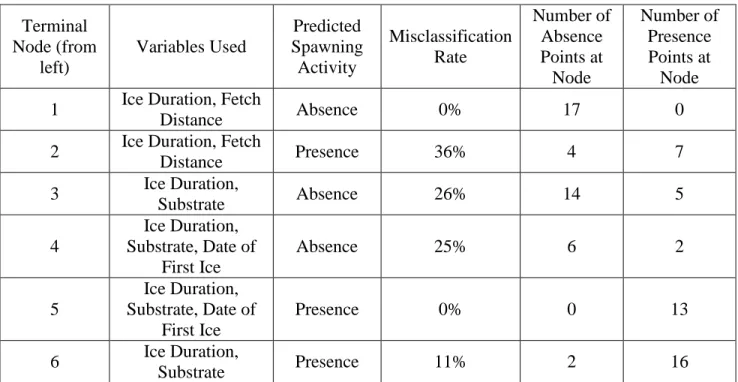
Table 9. CART training model results for Cisco with node classifications and misclassification rates. Terminal Node (from left) Variables Used Predicted Spawning Activity Misclassification Rate Number of Absence Points at Node Number of Presence Points at Node 1 Ice Duration, Fetch
Distance Absence 0% 17 0
2 Ice Duration, Fetch
Distance Presence 36% 4 7 3 Ice Duration, Substrate Absence 26% 14 5 4 Ice Duration, Substrate, Date of First Ice Absence 25% 6 2 5 Ice Duration, Substrate, Date of First Ice Presence 0% 0 13 6 Ice Duration, Substrate Presence 11% 2 16
Table 10. Classification accuracy for the Cisco random forest model.
Modeled Absence Modeled Presence Classification Error
Observed Absence 27 16 0.372093
30
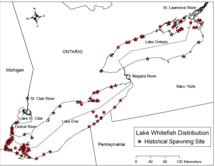
Fig. 1. Sites historically used for spawning by Lake Whitefish in Lake Erie, Lake Ontario, and connecting channels restricted to depths less than 25m.
31
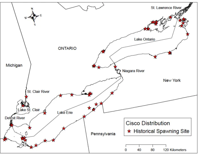
Fig. 2. Sites historically used for spawning by Cisco in Lake Erie, Lake Ontario, and connecting channels restricted to depths less than 25m.
32
Fig. 3. CART training model for Lake Whitefish showing fetch distance and ice cover duration as important variables. Green shaded boxes represent predicted presence while blue shaded boxes represent predicted absence. A lighter box color indicates a higher misclassification rate for that split. Misclassification rates for the split are listed as fractions, where the number of misclassified points is divided by the total number of points at the node. The final number in each box is the total percentage of points from the data set that are found in the node. The very top node shows that presence and absence sites in the data are divided 50/50.
33
Fig. 4. Output map from Lake Whitefish CART model highlighting predicted areas of spawning presence and absence across the study area.
34
Fig. 5. Importance of model variables for the Lake Whitefish random forest model ranked according to overall model accuracy when that variable is removed (left) and decrease in purity of the node when that variable is not considered in the division (right). Fetch distance and date of first ice were ranked as most important in the model for both measurements.
35
Fig. 6. Interaction plot from the Lake Whitefish random forest model showing that the highest probability for spawning presence (red spots) occur in regions where fetch distance is lower than approximately 30km and the date of first ice is between day 125 (December 25) and day 134 (January 3).
36
Fig. 7. Output map from Lake Whitefish random forest model highlighting predicted areas of spawning presence and absence across the study area.
37
Fig. 8. CART training model for Cisco showing ice duration, substrate, and distance from a stream order 6 tributary as important variables. Notation as in Figure 3.
38
Fig. 9. Output map from Cisco CART model highlighting predicted areas of spawning presence and absence across the study area.
39
Fig. 10. Importance of model variables for the Cisco random forest model ranked according to overall model accuracy when that variable is removed (left) and decrease in purity of the node when that model is not considered in the division (right). Ice duration was ranked as the most important variable for overall model accuracy, and ice duration and fetch were ranked as most important in the model for Gini index purity.
40
Fig 11. Interaction plot from the Cisco random forest model showing that the highest probability of spawning presence (red spots) occurs in regions where ice cover duration is between about 55 and 65 days. Spawning presence is predicted to be lowest when fetch distance is above
41
Fig. 12. Output map from Cisco random forest model highlighting predicted areas of spawning presence and absence across the study area.
42
Fig. 13. Combined results from Lake Whitefish and Cisco CART models highlighting areas where predicted spawning presence overlaps for both species.
43
Figure 14. Combined results from Lake Whitefish and Cisco random forest models highlighting areas where predicted spawning presence overlaps for both species.
44
Literature Cited
Assel, R., K. Cronk, and D. Norton. 2003. Recent trends in Laurentian Great Lakes ice cover. Climate Change 57:185-204.
Baldwin, N. A., R. W. Saalfeld, M. R. Dochoda, H. J. Buettner, and R. L. Eshenroder. 2006. Commercial Fish Production in the Great Lakes 1867–2000.
http://www.glfc.org/databases/commercial/commerc.php
Batiuk, R. A., D. L. Breitburg, R. J. Diaz, T. M. Cronin, D. H. Secor, and G. Thursby. 2009. Derivation of habitat-specific dissolved oxygen criteria for Chesapeake Bay and its tidal tributaries. Journal of Experimental Marine Biology and Ecology 381:S204-S215. Bennett, M. R. 2003. Ice streams as the arteries of an ice sheet: their mechanics, stability, and
significance. Earth-Science Reviews 61:309-339.
Berst, A. H., and G. R. Spangler. 1972. Lake Huron-the ecology of the fish community and man's effects on it. Great Lakes Fishery Commission Technical Report No.21. Ann Arbor, Michigan.
Bolland, J. D., L. J. Bracken, R. Martin, and M. C. Lucas. 2010. A protocol for stocking hatchery reared freshwater pearl mussel Margaritifera margaritifera. Aquatic Conservation: Marine and Freshwater Ecosystems 20:695-704.
Breiman, L., J. H. Friedman, R. A. Olshen, and C. J. Stone. 1984. Classification and regression trees. Wadsworth International Group, California.
Brown, R. W., W. W. Taylor, and R.A. Assel. 1993. Factors affecting the recruitment of Lake Whitefish in two areas of northern Lake Michigan. Journal of Great Lakes Research 19:418-428.
45
Burton, T. M., D. G. Uzarski, and J.A. Genet. 2004. Invertebrate habitat use in relation to fetch and plant zonation in northern Lake Huron coastal wetlands. Aquatic Ecosystem Health and Management Society 7:249-267.
Cutler, D. R., T. C. Edwards Jr., K. H. Beard, A. Cutler, K. T. Hess, J. Gibson, and J. J. Lawler. 2007. Random forests for classification in ecology. Ecology 88:2783-2792.
De’ath, G., and K. E. Fabricius. 2000. Classification and regression trees: a powerful yet simple technique for ecological data analysis. Ecology 81:3178-3192.
Edsall, T. A., and G. W. Kennedy. 1995. Availability of Lake Trout reproductive habitat in the Great Lakes. Journal of Great Lakes Research 21:290-301.
Elith, J., S. J. Phillips, T. Hastie, M. Dudik, Y. E. Chee, and C. J. Yates. 2011. A statistical explanation of MaxEnt for ecologists. Diversity and Distributions 17:43-57.
Eshenroder, R. L., C. R. Bronte, and J. W. Peck. 1995. Comparison of Lake Trout- egg survival at inshore and offshore and shallow-water and deepwater sites in Lake Superior. Journal of Great Lakes Research 21:313-322.
Eshenroder, R. L., P. Vecsei, O. T. Gorman, D. L. Yule, T. C. Pratt, N. E. Mandrak, D. B. Bunnell, and A.M. Muir. 2016. Ciscoes (Coregonus, subgenus Leucichthys) of the Laurentian Great Lakes and Lake Nipigon. Miscellaneous Publication 2016-01. Great Lakes Fishery Commission, Ann Arbor, Michigan, USA.
Fitzsimons, J. D. 1995. Assessment of Lake Trout spawning habitat and egg deposition and survival in Lake Ontario. Journal of Great Lakes Research 21:337-347.
Flavelle, L. S., M. S. Ridgway, T. A. Middel, and R. S. McKinley. 2002. Integration of acoustic telemetry and GIS to identify potential spawning areas for Lake Trout (Salvelinus namaycush). Hydrobiologia 483:137-146.
46
Forsythe, P. S., J. A. Crossman, N. M. Bello, E. A. Baker, and K. T. Scribner. 2012. Individual-based analyses reveal high repeatability in timing and location of reproduction in Lake Sturgeon (Acipenser fulvescens). Canadian Journal of Fisheries and Aquatic Sciences 69:60-72.
Franklin, J. 2009. Mapping species distributions: spatial inference and prediction. Cambridge University Press, Cambridge, UK.
Freeberg, M. H., W. W. Taylor, and R. W. Brown. 1990. Effect of egg and larval survival on year-class strength of Lake Whitefish in Grand Traverse Bay, Lake Michigan.
Transactions of the American Fisheries Society 119:92-100.
Frissell, C. A., W. J. Liss, C. E. Warren, and M. D. Hurley. 1986. A hierarchical framework for stream habitat classification: viewing streams in a watershed context. Environmental Management 10:199-214.
George, E. M., W. Stott, B. P. Young, C. T. Karboski, D. L. Crabtree, E. F. Roseman, and L. G. Rudstam. 2017. Confirmation of Cisco spawning in Chaumont Bay, Lake Ontario using an egg pumping device. Journal of Great Lakes Research 43:204-208.
Goforth, R. R., and S. M. Carman. 2005. Nearshore community characteristics related to shoreline properties in the Great Lakes. Journal of Great Lakes Research 31:113-128. Goodyear, C. S., T. A. Edsall, D. M. Ormsby-Dempsey, G. D. Moss, and P. E. Polanski. 1982.
Atlas of the spawning and nursery areas of Great Lakes fishes. U.S. Fish and Wildlife Service FWS/OBS-82/52.
Gunn, J. M. 1995. Spawning behavior of Lake Trout: effects on colonization ability. Journal of Great Lakes Research 21:323-329.
47
Hayden, T. A., T. R. Binder, C. M. Holbrook, C. S. Vandergoot, D. G. Fielder, S. J. Cooke, J. M. Dettmers, and C. C. Krueger. 2018. Spawning site fidelity and apparent annual survival of Walleye (Sander vitreus) differ between a Lake Huron and Lake Erie tributary. Ecology of Freshwater Fish 27:339-349.
He, Y., J. Wang, S. Lek-Ang, and S. Lek. 2010. Predicting assemblages and species richness of endemic fish in the upper Yangtze River. Science of the Total Environment 408:4211-4220.
Hondorp, D. W., E. F. Roseman, and B. A. Manny. 2014. An ecological basis for future fish habitat restoration efforts in the Huron-Erie corridor. Journal of Great Lakes Research 40:23-30.
James, G., D. Witten, T. Hastie, R. Tibshirani. 2013. An introduction to statistical learning with applications in R. Springer, New York.
Jude, D. J., S. A. Klinger, and M. D. Enk. 1981. Evidence of natural reproduction by planted lake trout in Lake Michigan. Journal of Great Lakes Research 7:57-61.
Koelz, W. 1929. Coregonid fishes of the Great Lakes. Bulletin of the U.S. Bureau of Fisheries. 43:297-643.
Kondolf, G. M. 2000. Some suggested guidelines for geomorphic aspects of anadromous salmonid habitat restoration proposals. Restoration Ecology 8:48-56.
Krabbendam, M., N. Eyles, N. Putkinen, T. Bradwell, and L. Arbelaez-Moreno. 2016. Streamlined hard beds formed by paleo-ice streams: a review. Sedimentary Geology 338:24-50.
Lane, J. A., C. B. Portt, and C. K. Minns. 1996. Nursery habitat characteristics of Great Lakes fishes. Canadian Manuscript Report of Fisheries and Aquatic Sciences No. 2358.
48
Lawler, G. H., 1965. Fluctuations in the success of year-classes of whitefish populations with special reference to Lake Erie. Journal of the Fisheries Research Board of Canada 22:1197-1227.
Leblanc, J. P., B. L. Brown, and J. M. Farrell. 2017. Increased Walleye egg-to-larvae survival following spawning habitat enhancement in a tributary of eastern Lake Ontario. North American Journal of Fisheries Management 37:999-1009.
Leopold, L. B., and T. Maddock. 1953. The hydraulic geometry of stream channels and some physiographic implications. U.S. Geological Survey Professional Paper No. 252. U.S. Government Printing Office, Washington, D.C.
Lewis, C. A., N. P Lester, A. D. Bradshaw, J. E. Fitzgibbon, K. Fuller, L. Hakanson, and C. Richards. 1996. Considerations of scale in habitat conservation and restoration. Canadian Journal of Fisheries and Aquatic Sciences 53:440-445.
Loftus, D. H. 1980. Interviews with Lake Huron commercial fishermen. Ontario Ministry of Natural Resources, Lake Huron Fisheries Assessment Unit Report 1-80, Owen Sound, ON.
Lu, G. Y., and D. W. Wong. 2008. An adaptive inverse-distance weighting spatial interpolation technique. Computers and Geosciences 34:1044-1055.
Lynch, A. J., W. W. Taylor, T. D. Beard Jr., and B.M. Lofgren. 2015. Climate change
projections for Lake Whitefish (Coregonus clupeaformis) recruitment in the 1836 Treaty Waters of the Upper Great Lakes. Journal of Great Lakes Research 41:415-422.
Mainella, A. M. 2016. Comparison of MaxEnt and boosted regression tree model performance in predicting the spatial distribution of threatened plant, Telephus Spurge (Euphorbia telephioides). ProQuest Dissertations Publishing, Miami University.