www.elsevier.com/locate/jmaa
A derivative-free optimization algorithm based
on conditional moments
✩Xiaogang Wang, Dong Liang
∗, Xingdong Feng, Lu Ye
Department of Mathematics and Statistics, York University, Toronto, Ontario, Canada M3J 1P3
Received 10 June 2006 Available online 7 November 2006
Submitted by Steven G. Krantz
Abstract
In this paper we propose a derivative-free optimization algorithm based on conditional moments for finding the maximizer of an objective function. The proposed algorithm does not require calculation or approximation of any order derivative of the objective function. The step size in iteration is determined adaptively according to the local geometrical feature of the objective function and a pre-specified quantity representing the desired precision. The theoretical properties including convergence of the method are pre-sented. Numerical experiments comparing with the Newton, Quasi-Newton and trust region methods are given to illustrate the effectiveness of the algorithm.
©2006 Elsevier Inc. All rights reserved.
Keywords:Optimization; Derivative-free; Conditional moment; Trust region
1. Introduction
Optimization has been playing an important role in many branches of science and tech-nology such as engineering, finance, probability and statistics (see, for example, [7,10,11,20], etc.). There are many optimization algorithms that have been developed to locate the optima of
✩ This work was supported by National Engineering and Science Research Council of Canada.
* Corresponding author.
E-mail address:[email protected] (D. Liang).
0022-247X/$ – see front matter ©2006 Elsevier Inc. All rights reserved. doi:10.1016/j.jmaa.2006.08.091
continuous objective functions. We are concerned with the maximization problem of a smooth functionf of several variables. Formally, we seek the solution of the following problem:
max
x∈Df (x), (1)
whereD⊂Rnis a bounded domain.
For an optimization problem with no constraint, one widely used method is the Newton method. For the Newton–Raphson algorithm, the iteration is defined by
xk+1=xk−αiG−i 1gi,
whereαi is the step size,gi is the gradient vector, andGi is the Hessian matrix. The Newton method converges fast in general and could be very efficient for smooth objective functions. How-ever, the Hessian matrix is rather difficult or impossible to obtain in many practical problems. To rectify this problem, the Quasi-Newton algorithm is proposed by Davidon [5]. The basic idea of the Quasi-Newton algorithm is to use an iterative matrixHito approximate Hessian matrixG−i 1. The BFGS Quasi-Newton method by Broyden [2]–Fletcher [6]–Goldfarb [8]–Shanno [17] has been proved reliable and efficient for the unconstrained minimization of a smooth function. Al-though the matricesHi’s are positive definite in theory, it is well known that they are often not the case especially for high-dimensional space due to rounding errors. Also, ill-conditioned matrices can cause serious numerical problems in practice. There are many modified versions of
New-ton method such as the Damped NewNew-ton method and theLavenberg–Marquardt type method
(see [7,13]). A polynomial-time algorithm for linear problems has also been proposed (see [4]). However, all these methods must require the calculation of the derivatives of objective functions. Another well-known problem with Newton method and the modified methods based on the Newton method is that the initial values are usually required to lie within a relatively small neighbourhood of the true optimum to ensure any desired accuracy. For example, one of the most widely used algorithms in statistics is the so-called Expectation–Maximization (EM) algorithm. It has been observed that this algorithm converges slowly and is very sensitive to the initial value. The problem lies in the maximization step of the algorithm in which the Newton or Quasi-Newton methods are employed (see [9]). Furthermore, some objective functions encountered in practice could be either very flat or have quite large first-order derivative near the global optima. This creates additional challenges to the Newton or Quasi-Newton type of algorithms as the accurate evaluation of the derivatives and the choice of step size are crucial.
On the other aspect, the derivatives of objective functions might not be available in many applications of maximization. Therefore, there have been considerable interests in developing effective algorithms that are of derivative-free. The trust region methods are widely studied and successful in the literature (see, for example, [12,15,19], etc.). For example, one of very recent trust region methods is called wedge trust region method (see Marazzi and Nocedal [12]). The wedge trust region method employs a model which interpolates the objective function at a set of sample points. The model is built upon the trust region framework such that the convergence of the model is guaranteed. Therefore, the model in wedge trust region method can be in either linear or quadratic order.
In this paper, we propose a novel derivative-free algorithm for the general optimization prob-lem based on conditional moments. The proposed algorithm is built upon a direct evaluation of the conditional moments of a non-negative function which represents the local centre of gravity of a mass function. The algorithm constructs a path defined by the geometric centres of the ob-jective function within a series small neighbourhoods so that it will travel dynamically towards the global optimum. The proposed algorithm is free of any order derivatives of the objective
functions and only depends on local integrations which are evaluated by the numerical quadra-tures such as the composite Simpson quadraquadra-tures and the composite quadraquadra-tures of Gaussian types. There are two iterative parameters in the procedure and they will be valued adaptively in the algorithm. For the proposed method, we have further established the theoretical properties including its convergence. Numerical experiments comparing with the Newton, Quasi-Newton and trust region methods are taken to illustrate the performance of the algorithm. It shows that the algorithm is very effective when the objective functions rise either very sharply or slowly near the global optimum. It is also very effective when there exist multiple local optima with a close proximity of global one.
The remaining part of the paper is organized as follows. In Section 2, we give a general description of the algorithm and we also describe the method of choosing the parameters adap-tively. Theoretical properties of the proposed method are established in Section 3. Numerical results comparing the proposed algorithm with the Newton, Quasi-Newton and wedge trust re-gion method are provided in Section 4. Finally, the conclusion is given in Section 5.
2. The derivative-free conditional moment algorithm 2.1. The basic idea
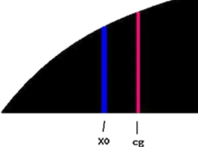
The idea of our derivative-free algorithm originated from the property of conditional mo-ments. The moments are defined in probability (see [1]), which can describe the local centre of gravity of a mass function. For simplicity, we assume that the objective function is positive everywhere. Then the objective function could be considered as a mass density function. Higher value of the objective function would provide more weight in its neighbourhood. For example, consider a symmetric objective function with the only optimum located at 0. The centre of func-tion coincides with the centre of gravity located at 0. In this simple example, finding the optimum is equivalent to finding the centre of gravity. However, for a non-symmetric non-negative func-tions, these two problems are no longer equivalent as the location of the global optimum often differs from the centre of the gravity. Thus instead of considering the centre of gravity for the entire objective function, we consider the local centre of gravity given a small neighbourhood. This corresponds to the first-orderconditionalmoment if the objective function is non-negative. Furthermore, we propose to move dynamically through a series of varying neighbourhoods and the movement is governed by a sequence of local gravity centres of these connected small local regions. Letx0represent the centre andcgrepresent the centre of gravity in this neighbourhood.
It is defined numerically as cg= xG(x) dx G(x) dx , (2)
whereG(x)is the non-negative mass density function. The centre of gravity defined by Eq. (2) coincides with the conditional first-order moment if the objective function is non-negative and can be normalized to 1. It can be seen that G(cg) > G(x0)which will be proved formally in
Section 3. Then, we can “relocate”x0tocgwhich occupies a higher “ground” within which the
average of objective function is bigger than that of the previous neighbourhood. This action is repeated until the required convergence is achieved.
This motivates us to define a derivative-free optimization method for solving the optimization problems. The detailed description of our algorithm will be given in the following subsections.
Fig. 1. The local centre of gravity in a monotone neighbourhood.
2.2. The method
In general, any real function F (x) can be decomposed into F+(x)=max(F (x),0) and
F−(x)=min(F (x),0). The positive partG(x)=F+(x)is of interest for maximization prob-lems. Thus we focus on non-negative functions in this article. IfF+(x)=0 for allx, we then set
F byF−CwhereC is a constant such thatG(x) >0 for somex.
Let the objective function G(x), x =(x1, x2, . . . , xn)∈Rn, be a non-negative continu-ous function, where n is the dimensionality. Then, for any givenα, x¯=(x¯1,x¯2, . . . ,x¯n)and
x=(x1, x2, . . . , xn)∈Rn, define a set Bx,¯ d(α)=x∈Rn: x− ¯x< d(α)⊂Rn (3) such that B(x¯,d(α)) G(y)dy=α, (4)
whered of the setB(x, d)¯ depends on the value ofα. Ifαis set to 0, thenB(x, d)¯ is a singleton set. To avoid this trivial case, we assume thatαk is positive in the sequel. It is obvious that the
value ofαis bounded byαM=
RnG(x) dx>0.
Then, we can propose the conditional moment method as follows: From the previous approx-imationxk with parameterαk>0 and radius parameterdk>0 obtained from (4) withx¯=xk, the new step approximation of the optima is defined as
xk+1=Txk, dk(αk) = 1 αk B(xk, dk) yG(y) dy, (5)
with initial guessx0 being given. The new positionxk+1is the ratio of the first-order moment over the zero-order moment on the local region. It is clear that the iteration at each stepk >0 only depends on the local integration overB(xk, dk). IfG(x)is a probability density function, thenxk+1 represents the conditional mean on B(xk, dk). Meanwhile, the new approximation
xk+1also depends the choice of the parametersαandd. 2.3. The algorithm
There is only parameterαkin the proposed method which will be selected dynamically. How-ever, the method requires integration over a local region such that Eq. (4) is satisfied. In practice,
the computational cost to determine such an area for high-dimensional objective function could be prohibitively high. One logical way of realistically handling integration on the setB(xk, dk)
is to apply Eq. (5) for each dimension individually while the rest of the coordinates are fixed. The coordinates of the location at thekth iteration, say,xk will then be updated one at the time in the same fashion of the well-known Gibbs sampler in physics and statistics (see [16]).
Therefore, we then seek to findrk=(r1k, r2k, . . . , rnk),i=1,2, . . . , n, such that
ηxk,rk= x1k+r1k x1k−r1k · · · xnk+rnk xk n−rnk G(x1, x2, . . . , xn) dx1dx2· · ·dxn−αk=0. (6)
Therik determines the lower and upper limits of integration onith dimension.
Thus, the set of parameters of our algorithms then becomes rk. Instead of finding rik us-ing exhaustive search, we propose to find a reasonable estimate of rik using a sequencetik(l),
l=1,2, . . ., as follows. Given an initial valuetik(0), we use an iterative method to find an ap-proximation ofrik as follows tik(l)=tik(l−1)− η(x k, tk i(l−1)) βk(xk, tk i(l−1)) , l >0, (7)
whereβk=∂η(xk,rk)/∂rik andl is the iterative number. For an iteration numberlN, we then approximaterikbytik(lN)(anddik=rik).
As it can be seen, the method of findingdik is based on the Newton method of finding roots
of equation in one dimension. We emphasize that both functionsη andβk do not involve any
evaluation of the derivative of the objective functionG. The formula for the high-dimensional case can be expressed in the same fashion.
For simplicity, we now state the algorithm using the proposed method for two-dimensional function.
Step 1. For a given(x1k, x2k)andαk, computetk
1(l)by the iterative numerical method defined by
Eq. (7) for approximatingd1k+1. Setd1k+1=t1k(lN)for a large value ofl, saylN. Step 2. Find the new value ofx1k+1by using Eq. (5) withαk andd1k+1obtained in Step 1. Step 3. Updateαk+1by using
α1Cor= xk1+d1k x1k−d1k x2k+d2k x2k−d2k x1−x1k+1+Sign∗(x1k+1−x1k) x1k+1+Sign∗(x1k+1−x1k) G(x1, x2) dx1dx2, (8)
where Sign=sign(x1k+1−xk1). Setαk+1=min(αk+αCor1 , αk1)ifαk+αCor1 >0. Step 4. Findd2k+1by usingt2k(l)in Eq. (7) withx1k+1obtained in Step 2 andαk+1obtained in
Step 3.
Step 6. Updateαk+1by using α2Cor= x1k+1+dk 1 xk1+1−dk1 x2k+1+dk 2 x2k+1−d2k x2−x2k+1+Sign·(x2k+1−x2k) x2k+1+Sign·(x2k+1−x2k) G(x1, x2) dx1dx2, (9)
where Sign=sign(x2k+1−x2k). Setαk+1=min(αk+1+αCor2 , αk+1)ifαk+1+α2Cor>0. Step 7. Repeat Steps 1–6 until convergence criterion is satisfied.
Remark.In the algorithm, the local integrations in Eqs. (8) and (9) are evaluated by numerical quadratures. For general objective functions, we can obtain accurate results by using the compos-ite Simpson quadrature. Furthermore, the Gaussian quadratures and the composcompos-ite quadratures of Gaussian types could obtain very effective and highly accurate values for high-dimensional functions (see [3,18]).
3. Theoretical properties of the method
In this section, we will establish the theoretical properties of the method. We prove that the algorithm will generate a sequencexk such thatG(xk)is a non-decreasing sequence. We also establish the convergence and convergence rate for the proposed algorithm.
3.1. Non-decreasing property in monotone neighbourhoods
We first show that the size ofB(x, d)is a non-decreasing function ofαfor any fixed position ofxk.
Lemma 3.1.Forα1, α2>0, let B(xk,d 1)G(y) dy=α1and B(xk,d 2)G(y) dy=α2. Ifα1> α2,
then for any givenx∈Rm,d(α1)d(α2).
Proof. For any givenα1andα2such thatα1> α2, let us assume thatd(α2)d(α1). By (4), it
follows that α2−α1= B(xk,d 2) G(y) dy− B(xk,d 1) G(y) dy = {y:d1y−xkd2} G(y) dy0.
The above inequality follows becauseG(x)0. This is a contradiction. 2
We can also show that the new estimate lies within the neighbourhood ofxk.
Lemma 3.2.For any givenα >0andxk, we have xk+1∈Bxk, d.
Proof. By the mean value theorem, it follows that 1 α B(xk,d) xG(x) dx=x∗k1 α B(xk,d) G(x) dx=x∗k, wherex∗k∈B(xk, d). 2
Then, we establish the first important property of the algorithm. The following theorem shows that our algorithm will generate a strictly increasing sequenceG(xk),k=1,2, . . . , n, if the deriv-ative is monotone in a local region. This implies that algorithm will try to move up to the local optimum. Although the derivative was not used in finding the direction, the algorithm can still find the direction such that it moves to a “higher” ground.
Theorem 3.1.For any givenαandxkand a continuous functionG(x), if∂G(∂xx)
i =0onB(x
k, d) fori=1, . . . , n, then
Gxk+1> Gxk. (10)
Proof. Observe that
x1k+1−x1kα = d −d d2−y2 1 −d2−y2 1 · · · d2−y2 1−···−y2n−1 −d2−y2 1−···−yn2−1 ·y1 G x1k+y1, x2k+y2, . . . , xnk+yn dyndyn−1· · ·dy1 = d 0 d2−y2 1 −d2−y2 1 · · · d2−y2 1−···−yn2−1 −d2−y2 1−···−y2n−1 y1 G x1k+y1, x2k+y2, . . . , xnk+yn −Gx1k−y1, x2k+y2, . . . , xnk+yn dyndyn−1· · ·dy1 = d 0 d2−y2 1 −d2−y2 1 · · · d2−y2 1−···−y2n−1 −d2−y2 1−···−yn2−1 y1dyndyn−1· · ·dy1 ·Gx1k+ξ1(1), xk2+ξ2(1), . . . , xnk+ξn(1)−Gx1k−ξ1(1), x2k+ξ2(1), . . . , xnk+ξn(1),
Let v(d)= d 0 d2−y2 1 −d2−y2 1 · · · d2−y2 1−···−y 2 n−1 −d2−y2 1−···−yn2−1 y1dyn· · ·dy1.
It is clear thatv(d)is positive.
It then follows that there existsξ(i)=(ξ1(i), ξ2(i), . . . , ξn(i))∈ {y∈Rn: yd andyi0},
i=2,3, . . . , n, such that xik+1−xik =v(d) α × G
xk1+ξ1(i), . . . , xik−1+ξi(i)−1, xik+ξi(i), xik+1+ξi(i)+1, . . . , xnk+ξn(i)
−Gx1k+ξ1(i), . . . , xik−1+ξi(i)−1, xik−ξi(i), xik+1+ξi(i)+1, . . . , xnk+ξn(i).
Since the objective function is monotone onB(xk, dk), therefore the sign of xik+1−xik is determined by whether the objective function is increasing or decreasing. Therefore,
∂G ∂xi
xk+θxk+1−xkxki+1−xki>0, (11) whereθ∈ [0,1],i=1, . . . , n.
By the Taylor expansion, we know that:
Gxk+1=Gxk+ n i=1 ∂G ∂xi xk+θxk+1−xkxik+1−xki, 0θ1. (12) It follows thatG(xk+1) > G(xk). 2
If the derivative is close to zero, the algorithm can still produce a strictly increasing sequence
G(xk),i=1,2, . . . , n, for some givenα. The next theorem formally establishes the result.
Theorem 3.2.Assume the following:
(i) The optimum is contained in a bounded and closed set O. For any givenε >0,D(ε)= O∩ni=1{x∈Rn: |∂x∂G
i(x)|ε}is closed; (ii) The partial derivatives ∂G(∂xx)
i is continuous with respect toxinR
n,i=1,2, . . . , n. Then, there existsα >¯ 0, such that for anyα∈(0,α¯], andxk∈D(ε),
Gxk+1(α)> Gxk(α).
Proof. For any given ε >0, D(ε) is bounded and closed. It follows that ∂G(∂xx)
i is uniformly
continuous inD(ε)with respect tox, i.e.∃δ(ε) >0 such that,∀x∈D(ε), ifx−x< δ, then
|∂G(x) ∂xi −
∂G(x) ∂xi |<
ε
2n. By assumption (ii),G(x)is continuous with respect tox inR
n. Then, ∀x∈D(ε), we define α(x)= y−xδ/2 G(y) dy. (13)
It follows thatα(x)is continuous with respect to x. We note thatα(x) >0. Otherwise, as-sume thatα(x)=0, i.e.y−xδ/2G(y) dy=0. SinceG(y)0, thenG(y)=0 for anyysuch thaty∈ {y∈Rn: x−yδ2}. Thus, ∂G∂x
i(x)=0,i=1,2, . . . , n, i.e.x∈R
n−D(ε). This is contradiction.
SinceD(ε) is bounded and closed, thereforeα(x)has a minimum value in the fieldD(ε),
sayα˜. Letx−yd¯G(y) dy= ˜α,x∈D(ε), thend(x)¯ δ/2,x∈D(ε). Note that x1k+1−x1k =1 α ¯ d(xk) − ¯d(xk) ¯ d(xk)2−y2 1 −d(x¯ k)2−y2 1 · · · ¯ d(xk)2−y2 1−···−yn2−1 −d(x¯ k)2−y2 1−···−y 2 n−1 ·y1G x1k+y1, x2k+y2, . . . , xnk+yn dyndyn−1· · ·dy1 =1 α ¯ d(x k) − ¯d(xk) ¯ d(xk)2−y2 1 −d(x¯ k)2−y2 1 · · · ¯ d(xk)2−y2 1−···−y 2 n−1 −d(x¯ k)2−y2 1−···−y2n−1 y1 G x1k, x2k+y2, . . . , xnk+yn +y1 ∂G ∂x1 x1k+θy1, x2k+y2, . . . , xnk+yn dyndyn−1· · ·dy1 =1 α ¯ d(x k) − ¯d(xk) y1 ¯ d2−y2 1 −d(x¯ k)2−y2 1 · · · ¯ d(xk)2−y2 1−···−yn2−1 −d(x¯ k)2−y2 1−···−yn2−1 ·Gx1k, x2k+y2, . . . , xnk+yn dyndyn−1· · ·dy1 +1 α ¯ d(xk) − ¯d(xk) ¯ d(xk)2−y2 1 −d(x¯ k)2−y2 1 · · · ¯ d(xk)2−y2 1−···−yn2−1 −d(x¯ k)2−y2 1−···−yn2−1 ·y12∂G ∂x1 xk1+θ (y1)y1, x2k+y2, . . . , xnk+yn dyn· · ·dy1, whereθ (y1)∈ [0,1]. Let h(y1)=y1 ¯ d(xk)2−y2 1 −d(x¯ k)2−y2 1 · · · ¯ d(xk)2−y2 1−···−yn2−1 −d(x¯ k)2−y2 1−···−y2n−1 ·Gx1k, xk2+y2, . . . , xnk+yn dyndyn−1· · ·dy2.
Sincehis odd function, thus− ¯d(x¯ k)
x1k+1−x1k= 1 α ¯ d(xk) − ¯d(xk) ¯ d(xk)2−y2 1 −d(x¯ k)2−y2 1 · · · ¯ d(xk)2−y2 1−···−yn2−1 −d(x¯ k)2−y2 1−···−y 2 n−1 ·y12∂G ∂x1 x1k+θ (y1)y1, x2k+y2, . . . , xnk+yn dyndyn−1· · ·dy1, whereθ (y1)∈ [0,1]. In general, we have xik+1−xik= 1 α ¯ d(xk) − ¯d(xk) ¯ d(xk)2−y2 1 −d(x¯ k)2−y2 1 · · · ¯ d(xk)2−y2 1−···−yn2−1 −d(x¯ k)2−y2 1−···−yn2−1 ·yi2·∂G ∂xi x1k+y1, x2k+y2, . . . , xik−1+yik−1, xik+θ (yi)yi, xki+1+yik+1, . . . , xnk+yn · dyndyn−1· · ·dy1, whereθ (yi)∈ [0,1]. For anyi, we define
Cd¯xk= ¯ d(xk) − ¯d(xk) ¯ d(xk)2−y2 1 −d(¯xk)2−y2 1 · · · ¯ d(xk)2−y2 1−···−y2n−1 −d(¯xk)2−y2 1−···−yn2−1 yi2dyn· · ·dy1. (14)
(a) First, consider the case in which it satisfies
i Bxk,d¯∩ x∈R: ∂G ∂xi xk=0 =φ. (15)
Without loss of generality, we assume that
Bxk,d¯∩ x∈R:∂G ∂x1 xk=0 =φ.
It suffices to only consider the following case in which
∂G ∂x1 xkε. (16) Since wheny∈B(xk,d)¯ ,|∂x∂G 1(y)− ∂G ∂x1(x k)|< 1 2nε, therefore ∂G ∂x1 (y) >2n−1 2n ε. (17) We then have xk1+1−xk1>1 α· 2n−1 2n ε ¯ d(xk) − ¯d(xk) ¯ d(xk)2−y2 1 −d(¯xk)2−y2 1 · · · ¯ d(xk)2−y2 1−···−y2n−1 −d(¯xk)2−y2 1−···−yn2−1 y12dyndyn−1· · ·dy1.
It then follows that xk1+1−xk1>1 α· 2n−1 2n ·ε·C ¯ dxk. (18)
By (15), there existsx(p)∈B(α, x¯ k), such that ∂x∂G p(x
(p))=0. Therefore, ify∈B(α, x¯ k), it then follows that
∂x∂Gp(y)=∂G ∂xp (y)− ∂G ∂xp xk+ ∂G ∂xp xk− ∂G ∂xp x(p) ∂G ∂xp (y)−∂G ∂xi xk+∂G ∂xp xk− ∂G ∂xp x(p)< ε 2n+ ε 2n= ε n. Since|∂x∂G p(y)|< 1 nεfory∈B(xk,d)¯ , therefore, xkp+1−xkp 1 α ¯ d(xk) − ¯d(xk) ¯ d(xk)2−y2 1 −d(¯xk)2−y2 1 · · · ¯ d(xk)2−y2 1−···−yn2−1 −d(¯xk)2−y2 1−···−y2n−1 yp2 ·∂G ∂xp xk1+y1, x2k+y2, . . . , xkp−1+ypk−1, xpk +θ (yp)yp, xpk+1+ypk+1, . . . , xkn+yndyndyn−1· · ·dy1 < 1 α 1 nε ¯ d(x k) − ¯d(xk) ¯ d(xk)2−y2 1 −d(x¯ k)2−y2 1 · · · ¯ d(xk)2−y2 1−···−y 2 n−1 −d(x¯ k)2−y2 1−···−y2n−1 yp2dyndyn−1· · ·dy1 = 1 α 1 nεC ¯ dxk.
LetE= {p|∂∂Gxp(xk)=0}. By Taylor expansion and (11),
Gxk+1−Gxk = ∂G ∂x1 xk+θxk+1−xkxk1+1−xk1+ n i=2 ∂G ∂xi xk+θxk+1−xkxki+1−xki >1 α· 2n−1 2n ε· 2n−1 2n ε·C ¯ dxk− p∈E ∂x∂Gpxk+θxk+1−xk·xpk+1−xpk >1 α· 2n−1 2n 2 ·ε2Cd¯xk−1 α· 1 nε·C ¯ dxk· 1 nε·(n−1) =1 α·ε 2·Cd¯ xk· 4n2−8n+5 4n2 .
(b) Second, ifB(xk,d)¯ ∪n
i=1{x∈Rn: ∂G∂xi(x
k)=0} =φ, since ∂G
∂xi is continuous, therefore, ∂G
∂xi(y) >0 (or<0), wherey∈B(x
k,d)¯ . By (11) and the Taylor expansion ofG(xk+1), we then
have Gxk+1−Gxk= n i=1 ∂G ∂xi xk+θxk+1−xkxik+1−xik >1 α·ε 2·Cd¯ xk· 4n2−8n+5 4n2 .
SinceC(d(x¯ k))is positive and 4n2−8n+5>0 whenn1. It then follows that
Gxk+1−Gxk>0. 2
The above theorem only characterizes the behaviour of the algorithm when the derivative is not zero or its absolute value is bounded from below. However, it does not provide any assurance that the algorithm will enter into a small neighbourhood of the optima. The following theorem in the next subsection shows that at least some of the estimates to the optima generated by the algorithm will have the first-order derivative that is close to zero.
3.2. Convergence of the method
In this part we will discuss the convergence theorems for our method. Basically, we prove that there exists a path of convergence to the true global optimum.
Theorem 3.3.Under the assumptions of Theorem 3.2, there exists a sub-sequence {xmk(α)}, whereα∈(0,α¯], which satisfies:Anyε >0,∃K(ε) >0, whenk > K(ε),xmk ∈D(ε)c, where D(ε)c=Rn−D(ε).
Proof. Assume that no such sub-sequence exists, then there must existM >0 such that when
m > M, we havexm∈D(ε). DenoteG(xm)byym. By Theorem 3.4, when m > M,{ym}is increasing.
Note thatGis continuous since it is differentiable. Since D(ε)is closed and bounded, thus
Gis bounded in D(ε). It then follows that the sequence{ym}is convergent. Denote the limit byy˜, we must haveyky˜whenk > M. SinceD(ε)is bounded, therefore{xm}has a convergent sub-sequence. Assume it is{xkl}. Denote the limit byx˜.D(ε)is closed, sox˜∈D(ε).
SinceGis continuous, we have
G(x)˜ =G lim l→∞x kl = lim l→∞G xkl= lim l→∞y kl = ˜y.
By Theorem 3.4,G(T (x, d(˜ α))) > G(¯ x)˜ , whereT is defined in (5).
Observe that G◦T is continuous with respect to x since G and T are continuous. Let
ε=G(T (x, d(˜ α)))¯ −G(x)˜ . Thus,∃L >0, s.t.l > L,|G(T (x,˜ α))¯ −G(T (xml, d(α)))¯ |< ε, i.e. G(xml+1)=G(T (xml, d(α))) > G(T (¯ x, d(˜ α)))¯ −ε=G(x)˜ .
Therefore,yml+1>y˜whenl > L. It is a contradiction. 2
Theorem 3.4.Under the assumptions of Theorem3.2, ifxk∈D(ε)whereD(ε)is defined as in Theorem3.2, then there exists a constantr∈(0,1)such that
G(x∗)−Gxk+1< r·G(x∗)−Gxk, (19)
whereGachieves its maximum value at the pointx∗. Proof. From the proof of Theorem 3.2, we know that:
Gxk+1−Gxk> 1 α·ε 2·Cdxk· 4n2−8n+5 4n2 .
Whenαfixed, then by the Theorem of Implicit Function, it follows thatdis continuous with respect tox,x∈D(ε). SinceD(ε)is closed and bounded, therefored has minimum value when
x∈D(ε), denoted byd0. LetC0=α1 ·ε2·C(d0)·(4n 2−8n+5 4n2 ). Thus,G(x k+1)−G(xk) > C 0. Note thatG(xk+1)G(x∗), so 0< C
0< G(x∗)−G(xk). Thus there existsc∈(0,1), s.t.C0=
c·(G(x∗)−G(xk)). Therefore,
0G(x∗)−Gxk+1< G(x∗)−Gxk−C0=r·
G(x∗)−Gxk,
wherer=1−c. 2
Lemma 3.3.Letx∗be the maximizer ofGand∇G(x∗)=0. If the functionG(·)is twice contin-uously differentiable and there exist constants0< mM <∞such that for allx,y∈Rn,
−My2y, Gxx(x)y
−my2, (20)
then, we must have m
2x
∗−x2G(x∗)−G(x)M
2 x
∗−x2, (21)
wherex∗is the maximizer ofG(x). Proof. Note that
G(x)−G(x∗)=∇G(x∗), (x−x∗)+1 2 x−x∗, Gxx x+θ (x−x∗)(x−x∗) for someθ∈ [0,1]. 2
Finally, we can prove that the algorithm convergesR-linearlybefore enteringDc(ε). Detailed discussions on different rate of convergence for algorithms can be found in Polak [14].
Theorem 3.5.Suppose the assumptions in Theorem3.2and Lemma3.3hold. Letε¯ andD(ε) be the same as defined in Theorem3.2. Let {xk(α)}be a sequence defined by our algorithm, where α∈(0,α¯]. If xk ∈D(ε) for kK, then there exists c∈(0,1), s.t. x∗−xk< ck[m2(G(x∗)−G(x0))]1/2, wherex∗is the maximizer of the functionG(x).
Proof. From Theorem 3.4, we know that∃r∈(0,1), s.t.G(x∗)−G(xk+1) < r·(G(x∗)−G(xk)). By Lemma 3.3, it follows thatm2x∗−xk+12G(x∗)−G(xk+1) < r·(G(x∗)−G(xk)). It fol-lows by recursion that, forkK,
m
2x
∗−xk+12
3.3. Results for unimodal functions
In this subsection, we now consider functions that are unimodal. Letx∗be the maximum for a unimodal function and define
E(ε)= x∈Rn: ∂G ∂xi (x)2n+1 2n ε, i=1, . . . , n . (22)
We also define a family of sets:N (x∗, ε)= {B⊂ ¯E(ε): x∗∈BandBis connected}. Obviously,
N (x∗, ε)is connected and closed, denoted byU (x∗, ε). Therefore,E(ε)¯ =U (x∗, ε)∪(E(ε)¯ − U (x∗, ε))andU (x∗, ε)is the maximum connected sub-set ofE(ε)¯ which includes the pointx∗. Define ME/U(ε)= sup x∈E(2n2+n1ε)−U (x∗,2n2+n1ε) G(x), mU(ε)= inf x∈U (x∗,ε)G(x). Furthermore, we define A(x∗, ε)=t: mU(ε) < t < G(x∗) , (23) B(x∗, ε)=t: ME/U(ε) < t < G(x∗) . (24)
Theorem 3.6. Under the assumptions of Theorem 3.2, if the function G is unimodal and
∃ε∗>0, s.t. G(x) >0 wherex∈U (x∗,2n2+n1ε∗), then given0< ε < ε∗ and any initial point x0∈ G−1(B(x∗, ε)), there exists α¯, ∀α∈(0,α¯], such that there exists K(ε,x0) >0, when k > K(ε,x0),G(xk)mU(ε).
Proof. SinceGis unimodal, we then have∃ε0>0,U (x∗,2n2+n1ε)is bounded whenε < ε0.
Let ε¯ = min{ε0, ε∗}. Since U (x∗,2n2+n1ε)¯ is closed and bounded, therefore D(ε)¯ ∪
U (x∗,2n2+n1ε)¯ is bounded and closed whered¯andD(ε)¯ are defined in Theorem 3.2.
We can findα >¯ 0 andd¯as described in Theorem 3.2. It follows that, for anyα∈(0,α¯], and for allx∈D(ε)¯ ∪U (x∗,2n2+n1ε)¯ , ifx−x<d¯, then
∂G(x∂xi)−∂G(x) ∂xi < ε¯ 2n (25) fori=1,2, . . . , n.
Observe thatx0∈U (x∗,2n2+n1ε)¯ ∪D(ε)¯ sincex0∈G−1(B(x∗,ε))¯ .
(1) We first considerx0∈D(ε)¯ . By Theorem 3.2, it follows that{xk}is an increasing sequence onD(ε)¯ . This implies thatG(xk) > mU(ε)¯ before the sequence entersE(¯ ε)¯ . Therefore, by Theorem 3.5,∃K >0, s.t.xK∈U (x∗,2n2+n1ε).
(2) Next we considerxK+1.
(i) IfxK+1∈U (x∗,2n2+n1ε)¯ , we then haveG(xK+1)F (ε). (ii) IfxK+1∈D(ε)¯ , therefore|∂x∂G i(x K+1)|<2n+1 2n ε¯since| ∂G ∂xi(x K)−∂G ∂xi(x K+1)|< ε¯ 2n and |∂G ∂xi(x
K)|<ε¯. Then it follows that G(xK+1)m
U(ε)¯ . Note thatG(xk+1) > G(xk)if
xk∈D(ε)¯ .
For any sequence{αk}, we can define a new sequence{xk}, wherexk is defined as: xk(αk)= 1 αk y∈B(dk) yG(y) dy. (26)
If the functionGis unimodal and the optima is unique, the next theorem proves that there is a sequence that converges to the maximizer.
Theorem 3.7.If the conditions in Theorem3.6hold, and if∃ε(1)>0, onlyx∗satisfies∂x∂G i(x)=0, i=1, . . . , n, inU (x∗, ε(1)), then∃ε(2)>0, any initial pointx0, wherex0∈G−1(B(x∗, (2))), for anyε∈(0, ε(2)], we can find a sequence{αk}s.t. the sequence{xk(αk)}converges tox∗.
Proof. Since G is unimodal, therefore∃ε(3)>0, s.t.mU(ε)ME/U(ε), when ε < ε(3). Let
¯
ε=min{ε(1), ε(2), ε(3), ε∗}, whereε∗is defined in Theorem 3.6.
Note that ME/U(ε) is non-increasing with respect to ε if G is unimodal. It then follows
that ∃K >0, s.t. K1 < ε, where εε¯. By Theorem 3.6, we know that, for any given x0∈ G−1(B(x∗, ε)),ε∈(0,ε¯], there∃α(1)>0 and∃k1>0, s.t. whenk > k1,xk(α(1))mU(K1). Since ME/U(K1+1)ME/U(K1)mU(K1), therefore xk1 ∈G−1(B(x∗,K1)). It follows that
∃α(2)>0 and∃k2>0, s.t. whenk > k2+k1,xk(α(2))mU(K1+1). In general, it follows that there existsα(m)>0 and∃km>0, s.t. whenk > km+km−1+ · · ·+k1,xk(α(m))mU(K+1m−1). Setαk=α(i), whenki< kki+1. Consequently, we can define the sequence{xk(αk)}. Let
Ψm= {G−1(A(x¯ ∗,K+1m))},m=1,2, . . .. SinceG−1(A(x∗,K1))⊃G−1(A(x∗,K1+1))⊃ · · · ⊃
G−1(A(x∗,K+1m))⊃ · · ·, limm→∞F (K+1m−1)=G(x∗) and G is unimodal and continuous, thereforeΨm= {x∗}. It then follows that limk→∞xk=x∗. 2
Finally, we study the relationship of the proposed derivative-free algorithm and a general gradient algorithm. We obtain the following theorem.
Theorem 3.8.If the second partial derivative ofG(x)exists, then for any givenα >0, we have xk+1=xk+ n n+2 ∇G(xk) G(xk) d 2 k +O dk3, (27) wheredk satisfies B(xk,d)G(xk) dx=α.
Proof. To simplify the notation, letx0=xk andxk+1=T (xk)whereT is the operator defined
by Txk=1 α B(xk,d) yG(y) dy. (28)
Lety=x0+u. It then follows that
T (x0)= 1 α B (x0+u)G(x0+u) du =1 α x0 B G(x0+u) du+ B uG(x0+u) du =x0+ 1 αM(x0),
where T (x0)= B uG(x0+u) du, (29) andB= {u∈Rn: ud}.
Expand the density function as follows:
G(x0+u)=G(x0)+u∇G(x0)+ u2Q(x0+tu), 0< t <1, where Q(x0+tu)= 1 2! n i=1 n j=1 yiyj ∂2f ∂xi∂xj x=x0+tu . (30)
By using polar coordinates, it can be verified that
B du=d n nCn, B udu=0, B u2du= d n+2 n+2Cn, whereCn=( √ π )n−2 Γ (n2) 2π. We then have α= B G(x0+u) du = B G(x0) du+ B u∇G(x0) du+ B u2Q(x0+tu) du =α0+α1+α2, where α0=G(x0) dn n Cn, α1= ∇G(x0) B udy=0, α2= B u2Q(x0+tu) duMB dn+2 n+2Cn, whereMB=maxB∂ 2G(x 1,x2,...,xn) ∂xi∂xj for anyi, j. This implies that
α=G(x0)
dn n Cn+O
Similarly, we obtain that M(x0)=I0+I1+I2, (32) where I0=G(x0) B udu=0, I1= ∇G(x0) B u2du= ∇G(x0) dn+2 n+2Cn, I2= B uu2Q(x0+tu) du=O dn+3.
It then follows that
M(x0)= ∇G(x0) dn+2 n+2Cn+O dn+3. We then have 1 αM(x0)= n n+2 ∇G(x0) G(x0) d2+Od3.
Moreover, if we ignore the higher order terms in Eq. (27), we then have
xk+1=xk+ n n+2 ∇G(xk) G(xk) d 2 k. 2 (33)
If the limit of the sequencexk exists, sayx∗, by taking the limit on both sides of the above equation, we then have
x∗=x∗+ n n+2 ∇G(x∗) G(x∗) d 2 k.
It then implies that∇G(x∗)=0. Therefore, this algorithm is also trying to find saddle points whose first-order derivative equal to zero.
Although the first-order derivative is not used in the proposed algorithm, the moving direction of the algorithm is actually closely related to the gradient. For simplicity, let us consider the 1-dimensional case. Iff(xk) >0, then the second term in Eq. (33) will be positive. This implies that the xk+1 is generated to the right of xk which moves to a “higher” ground. Otherwise,
xk+1will move to the left ofxk. Therefore, the first-order derivative actually dictates the direction of the next move. We emphasize that the first-order derivative is never calculated.
Although we have established convergence properties in this section, we remark that conver-gence to a local optimum is still possible in our algorithm. For example, for a very small initial
value ofα, our algorithm could converge to a local optimum. However, we will show through
examples in the next section that the outcome of our algorithm is not very sensitive to the choice of the initial values.
4. Numerical experiments
In this section, we will present results of numerical experiments and compare our algorithm
with three widely used algorithms:the Newton,the Quasi-Newtonandthe wedge trust region
4.1. Comparison with Newton and Quasi-Newton method The first objective function that we consider is the following:
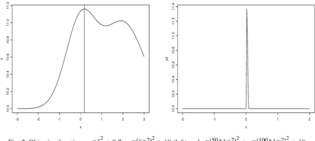
G11(x)=e−x 2
+0.7∗e−(x−2)2+10, −∞< x <∞. (34) This function is asymmetric and has one global maximum at 0.18 but with an additional local optima around 2. It is mainly flat on most of its domain but has a steep increase near the global and local optima. The function is displayed in the left panel of Fig. 2.
Table 1 provides a comparison between the Newton method and our algorithm. It can be seen that Newton method is very sensitive to the initial values. The Newton method could generate correct results when the initial values are set within the interval (−0.5,0.5). For other initial values, however, the Newton method does not work well. For example, it is interesting to exam the result generated by the Newton method when the initial value is 1. The location of this particular initial value is actually closer to the global optimum located at 0.18 than the local optimum at 2. However, the Newton method converges to the local saddle point 1.18 instead. If the initial values are set to be on the other side of the local optimum, then the Newton algorithm will be trapped at the local optimum. Furthermore, if the initial values are set to be either−1 or 3 which are both relatively far from the optimum, then the Newton method could not calculate the derivatives at those locations and consequently failed to find either the global or local optima. Among all the initial values we tried, the Newton method could only find the global optima when the initial values are very close to the true global maxima. Another commonly used optimization algorithm for one-dimensional case is theSecantmethod. The Secant method does not require the calculation of the derivative. But it does require the input of 2 parameters. Table 1 also provides the results using different initial values for the Secant method. It can be seen that the Secant method also suffers the similar drawback as the Newton method. First of all, it could also diverge as the Newton method does. Secondly, the accuracy of the algorithm depends heavily on the initial choice of the parameters.
In contrast with the results generated by the Newton method, our algorithm based on condi-tional moments (CM) can find the global optima regardless of the relative position of the initial value to the global optima. In particular, our algorithm gives a very surprising performance when the initial value is set to be 3. In this case, the starting point lies on the right-hand side of both the global and the local optima. Our algorithm actually jumped across the local optimum and indeed reached the global optimum.
Table 1
Comparison with Newton and Secant method for functionG11(tolerance=10−8)
Initials x0= −1 x0= −0.5 x0=0.0 x0=0.5 x0=1.0 x0=2.5 x0=3 Newton NA 1.1808 0.1791 0.1791 1.1808 1.8948 NA CM 0.1806 0.1824 0.1803 0.1812 0.1813 0.1813 0.1813 Initials (−1,−0.5) (−1,0) (−0.5,0) (−0.5,1) (0.5,1.0) (0.5,1.5) (1,2) (1,2.5) Secant NA 0.1791 0.1791 1.1808 1.1808 1.1808 1.8948 NA Table 2
Comparison with Newton and Secant method for functionG12(tolerance=10−8)
x0=0 x0=0.01 x0=0.02 x0=0.03 x0=0.04 x0=0.05
Newton NA NA 0.0229 0.0229 NA NA
CM 0.0224 0.0224 0.0227 0.0.234 0.0229 0.0229
(0,0.01) (0,0.03) (0.01,0.02) (0.01,0.03) (0.02,0.04) (0.03,0.04) (0.03,0.05)
Secant NA 0.0221 0.0221 NA NA NA −0.1282
The second objective function we used is
G12(x)=exp
−(50x−2)2+exp−(100x−2)2+100, −∞< x <∞. (35) This function has one unique optimum at 0.022 but is very steep in its neighbourhood. It is plotted in the right panel in Fig. 2.
The results of the Newton method and ours are presented in Table 2. We see that the depen-dence on the initial values is quite evident for the Newton method. In fact, the Newton method failed to produce any sensible results unless the initial values are set to be very close to the true optima. The results obtained through the Secant method are also given in Table 2. It can be seen that the Secant method is either divergent or failed to find the true optimum for most initial val-ues we selected. It is highly sensitive to the initial choice of the parameters. For example, the true optimum is found by using initial parameters(0.01,0.02). However, the Secant method is divergent for a similar pair of parameters, namely(0.01,0.03).
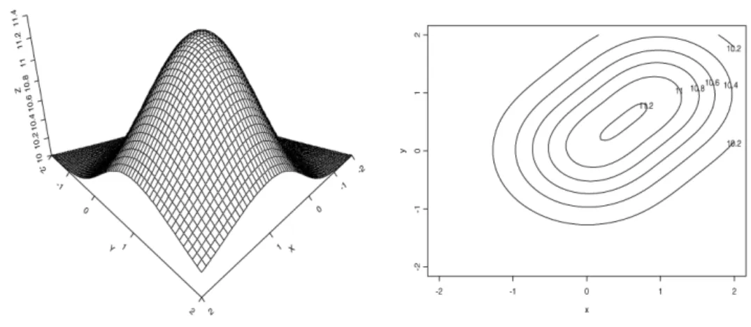
We now compare the performances of the Newton method and our method for a two-dimensional function:
G21(x, y)=e−(x 2+y2)
+e−(x−1)−(y−1)2+10, −∞< x <∞. (36) The above function has one unique optimum at(0.5,0.5). Unlike the functions studied in the one-dimensional case, this function is rather flat near the optimum as seen in Fig. 3.
In the two-dimensional case, Quasi-Newton method is also commonly used. We present the results from the Newton, Quasi-Newton and our methods (CM) in Table 3. It is clear that the Newton method is highly sensitive to the initial value of(X0, Y0). In fact, the Newton method
failed to perform any iteration in many initial values since the method could not calculate the derivatives of the objective function. In comparison, the Quasi-Newton method is only marginally better. Although it delivers the optimum in two cases in which the Newton method failed, the reported values are both grossly far from the true optimum. The Quasi-Newton method, however, would diverge for many initial values. In comparison, our method finds the true optima for most of the initial values. When the initial values are both negative, however, our method reports that the optimum is around(0,0). Although it seems that our method also missed the target for these cases, carefully examination of the objective function especially the contour plot in Fig. 3 reveals that the optimal value returned by our method is about 11 while the true optimal value
Fig. 3. Surface and contour plot for the functionG21.
Table 3
Comparison with Newton and Secant method for functionG21(tolerance=10−8)
(X0, Y0) Newton Quasi-Newton CM (−1.0,−1.0) NA NA (−0.00716,−0.00725) (−0.5,−0.5) NA (−4.0998,−4.0998) (−0.00347,−0.00381) (0.6,0.6) (0.50000,0.50000) (0.5000,0.50000) (0.50001,0.50001) (1.0,1.0) (0.50000,0.50000) (0.50000,0.50000) (0.50000,0.50000) (1.2,1.2) (0.50000,0.50000) (0.5000,0.50000) (0.50001,0.50001) (1.5,1.5) NA (5.09988,5.09988) (0.50000,0.50000) (2.0,2.0) NA NA (0.50000,0.50000) (3.0,3.0) NA NA (0.50000,0.50000)
for the function is 11.2. Our method could not proceed further since the top of the 2-dimensional function is very flat indeed. Thus those output results by our method seem to be quite reasonable given the nature of the function near the global optimum.
4.2. Comparison with wedge trust region method
We now compare our method with the wedge trust region method (see Marazzi and Nocedal [12]). The wedge trust region method has been shown to be very efficient and accurate for a variety of functions. We indeed apply the wedge trust region method to the functions studied in previous section. The wedge trust region works almost perfectly for those functions with very large or very small first-order derivatives. We proceed to make further comparison in much more complicated situations in which the global optima of the objective functions are accompanied by some local optima.
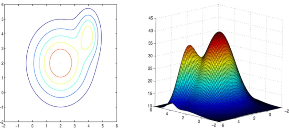
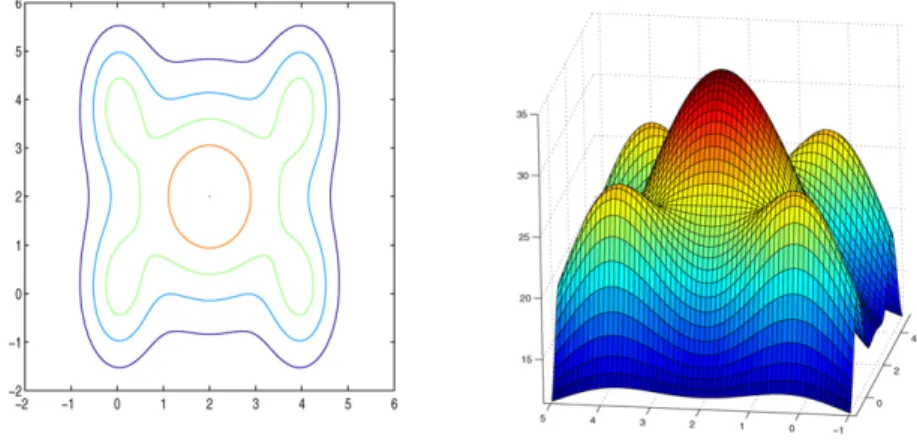
The first objective function we chose is the function
G22(x, y)=30 exp
0.01∗ −30(x−2)2−20(y−2)2
+20 exp−20(x−4)2−5(y−4)2+10.
The surface and contour plots are provided in Fig. 4. The global optimum is at(2,2)with a local optimum located at(4,4). We apply both the wedge trust region method and our method to this function. The results are presented in Table 4. We actually tried many initial values and many of those pairs give almost identical results for both methods. Thus, we only present results that
Fig. 4. Comparison with wedge trust method usingG22.
Table 4
Comparison between the wedge trust region method and the conditional moment method usingG22
Initial values Wedge trust region Conditional moment
(4,1) (2.000405,2) (2.004554,2.003649) (1,5) (2.000405,2) (2.005478,2.004500) (1,−1) (2.000405,2) (2.006220,2.005184) (1,1) (2.000405,2) (2.000781,2.000408) (0,4) (2.000405,2) (2.005800,2.004797) (5,5) (3.923584,4) (2.001318,2.000835) (4,6) (3.923584,4) (2.001557,2.001029) (3,5) (3.923584,4) (2.002954,2.002219) (5,3) (3.923584,4) (2.002939,2.002206)
are representative. The class of top four cases presented in Table 4 demonstrates that these two methods could both find the global optimum for this set of different starting points. If the location of the initial value is not close to the local optimum located at (4,4), the wedge trust region method is very effective and accurate. In fact, it is more efficient and accurate than our method. For example, if the starting point is chosen at(1,1)or(0,4), the wedge trust region locates the true global optimum very accurately while the CM method only converges to the neighbourhood of the location(2.005,2.005). However, if the initial values are chosen to be close to the local optimum at (4,4)such as those chosen in the last 4 cases in Table 4, the wedge trust region method will converge to the local optimum instead of the global one. Our CM method, however, converges successfully to the global optimum and ignored the attraction from the local optimum. In summary, the performance of the wedge trust region method also depends on the choice of the initial starting point. Our method, on the other hand, does not rely on the initial value and seem to be more robust although it could be less accurate than the wedge trust region method for some cases.
To further verify our observation that the wedge trust region method might be trapped in a local optimum which is close to the global one, we consider the following function:
G23(x)=30 exp
0.01∗ −30(x−2)2−20(y−2)2
Fig. 5. Surface and contour plot ofG23.
Table 5
Comparison between the wedge trust region method and the conditional moment method using functionG23
Initial values Wedge trust region Conditional moment
(2,5) (2.000000,2.0) (2.000000,2.000003) (2,−3) (2.000000,2.0) (2.000000,1.999999) (−2,2) (2.000000,2.0) (2.000001,2.000000) (2,−1) (2.000000,2.0) (2.000000,1.999998) (5,−1) (3.902682,0.2) (2.000001,1.999999) (5,5) (3.902682,4.0) (2.000000,2.000004) (−1,−2) (0.009731,0.2) (2.000000,1.999974) (−1,5) (0.009731,4.0) (1.999999,2.000001) (5,2) (3.902682,4.0) (2.000001,2.000000)
The surface and contour plots are given in Fig. 5. As we can see that the global optimum located at(2,2)is surrounded by four local optima. This is a more challenging case as the objective function changes more radically around the global optimum. We see that both methods would converge to the global optimum if the starting points are in one of the four “valleys.” This is not surprising as there exists a clear direct path to the optimum from those locations. However, the wedge trust region method would converge to one of the four local optima if the initial values are close to one of those local optima. In comparison, the CM method could jump over the local optimum nearby and go directly to the global optimum.
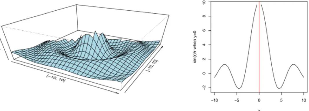
We also tried to compare our algorithm with the trust region algorithm for a very challenging function
G24=103sin(r)/r, (37)
wherer=x2+y2and−10< x <10,−10< y <10.
The optimum is achieved at the(0,0)which is the location of singularity of the derivative. Around the global optimum, there is also a ring of infinite local multi-optima within the range of[−10,10] × [−10,10].The graphical presentation of this function is shown in Fig. 6. The left panel shows the 3-D picture of the function with the singularity removed. The sectional plot of the function fory=0 is provided in the right panel of Fig. 6. Please note that the optimum has