T
HE
W
ILLIAM
D
AVIDSON
I
NSTITUTE
AT THE UNIVERSITY OF MICHIGANDeterminants of House Prices
in Central and Eastern Europe
By:
Balázs Égert and Dubravko Mihaljek
William Davidson Institute Working Paper Number 894
October 2007
Determinants of House Prices
in Central and Eastern Europe
Balázs Égert♣ Dubravko Mihaljek♦1
Abstract
This paper studies the determinants of house prices in eight transition economies of central and eastern Europe (CEE) and 19 OECD countries. The main question addressed is whether the conventional fundamental determinants of house prices, such as GDP per capita, real interest rates, housing credit and demographic factors, have driven observed house prices in CEE. We show that house prices in CEE are determined to a large extent by the underlying conventional fundamentals and some transition-specific factors, in particular institutional development of housing markets and housing finance and quality effects.
Keywords: house prices, housing market, transition economies,
central and eastern Europe, OECD countries
JEL classification: E20, E39, P25, R21, R31
♣ OECD Economics Department; CESifo; EconomiX at the University of Paris X-Nanterre and the William
Davidson Institute at the University of Michigan. E-mail: balazs.egert@oecd.org and begert@u-paris10.fr.
♦ Bank for International Settlements, Basel, Switzerland. E-mail: dubravko.mihaljek@bis.org.
1 The views expressed in this paper are those of the authors and do not necessarily represent the views of the
institutions the authors are affiliated with. We are thankful for helpful comments on earlier drafts to Peter Backé, Václav Beran, Claudio Borio, Dietrich Domanski, Luci Ellis, Jan Frait, Miroslav Singer, Greg Sutton, Paul Wachtel, Haibin Zhu, two anonymous referees and participants of seminars at the BIS, the Czech National Bank, the ECB and the Oesterreichische Nationalbank. We would also like to thank
Ljubinko Jankov, Gergő Kiss, Luboš Komárek, Davor Kunovac, Miha Leber, Mindaugas Leika, Andreja
Pufnik and Marjorie Santos for help in collecting the data for CEE countries. A version of this paper was
published in Comparative Economic Studies, 49(3), 367-388. Égert was with the Oesterreichische
Nationalbank when this study was written. Part of this study was prepared when Égert was visiting the Czech National Bank in 2006.
INTRODUCTION
Housing markets have revived strongly in many countries around the world in recent years, including in central and eastern Europe (CEE). Although house prices in this region remain on average far below western European levels, they have been catching up rapidly, with sustained real annual increases in the double-digit range not uncommon. The run-up in house prices has coincided with unprecedented expansion of private sector credit in the region, with loans for house purchases playing a key role in the expansion. This has raised concerns about financial stability implications of developments in the housing market, should house price dynamics become somehow disconnected from developments in the underlying fundamentals of housing demand and supply.
The determinants of house prices in CEE have not yet been systematically researched. To our knowledge, this is the first paper that tries to fill this void. Our main goal is to assess quantitatively whether the conventional fundamental determinants of house prices, such as disposable income, interest rates, housing credit and demographic factors, have played a role in the observed house price dynamics. Our model of the determinants of house prices draws on the standard variables used in the empirical literature, and also takes account of some transition-specific factors, such as the profound transformation of housing market institutions and housing finance in CEE, improvements in the quality of newly constructed housing, and growing demand for housing in this part of Europe by residents from other parts of Europe. In our empirical work we take a comparative approach and study the determinants of house price changes for various panels composed of transition economies and developed OECD countries. We use the mean group panel dynamic OLS (DOLS) estimator, which allows for cross-country heterogeneity in both short-run and long-run elasticities of house prices with respect to their determinants. The use of these panels provides insights into the common determinants of house prices for the two groups of countries and, at the same time, allows us to identify some important differences. Our main result is that, overall, per capita GDP, real interest rates, credit growth, demographic factors and indicators of institutional development of housing markets and housing finance are important determinants of house prices in CEE. The outline of the paper is as follows. The next section provides a brief overview of the theoretical and empirical literature on the determinants of house prices, and stylised facts on the dynamics and determinants of house prices in CEE and industrial countries. The subsequent section discusses the data issues, presents our empirical model and describes the estimation techniques. The following section presents the estimation results. Finally, the last section draws presents concluding remarks.
DETERMINANTS OF HOUSE PRICES
Theoretical model and empirical literature
House price dynamics are usually modelled in terms of changes in housing demand and supply (see eg HM Treasury, 2003). On the demand side, key factors are typically taken to be
expected change in house prices (PH), household income (Y), the real rate on housing loans
(r), financial wealth (WE), demographic and labour market factors (D), the expected rate of
return on housing (e) and a vector of other demand shifters (X). The latter may include
proxies for the location, age and state of housing, or institutional factors that facilitate or hinder households’ access to the housing market, such as financial innovation on the mortgage and housing loan markets:
) , , , , , , (P Y rWE D/ e X f DH H + − + + − + − = (1)
The supply of housing is usually taken to depend on the profitability of the construction business, which can in turn be described as a positive function of profitability that in turn
depends positively on house prices and negatively on the real costs of construction (C),
including the price of land (PL), wages of construction workers (W) and material costs (M):
) ) , , ( , ( − + = f P C P W M SH H L (2)
Assuming that the housing market is in equilibrium, with demand equal to supply at all times, house prices could be expressed by the following reduced-form equation:
) ) , , ( , , , , , , ( / + + − + + − + = f Y rWE D e X C P W M PH L (3)
The view that both the supply and demand for housing interact to determine an equilibrium level for real house prices should not be taken to imply that house prices are necessarily stable. In many countries it is frequently observed that house prices are significantly more volatile than would be predicted by the variation in the main determinants of supply and demand alone. Moreover, the structure of housing finance, spatial effects and tax treatment of owner occupancy may significantly affect house price dynamics in the long term.
The empirical literature using this framework is vast. Recent cross-country studies that are relevant for this paper (for the euro area, groups of industrial countries, and small European countries) include Annett (2005), Ayuso et al (2003), Girouard et al (2006), Sutton (2002), Terrones and Otrok (2004) and Tsatsaronis and Zhu (2004) (see Table A1 in Appendix). These studies generally find that the estimated elasticities of real house prices with respect to economic fundamentals differ widely, depending on the sample of countries, the period examined, and the methodology used. Nevertheless, two common patterns seem to emerge. First, key elasticities are higher for smaller countries (such as Denmark, Finland, the Netherlands and Norway) and catching-up economies (eg Ireland and Spain), than in the samples that include large industrial countries. Second, in addition to real income and real interest rates, credit growth, demographics and supply-side factors also play an important role in house price dynamics.
House prices and macroeconomic fundamentals in CEE and industrial countries
Real estate company data collected by the European Council of Real Estate Professions indicate that in 2005 average house prices per square metre in the capital cities varied from 800–900 euros in Bulgaria and Lithuania; to 1,100–1,300 euros in Hungary, Poland and the Czech Republic; to around 2,000 euros in Croatia and Slovenia. This compares with average house prices ranging in the same year from around 1,500 euros in Germany, Belgium and Austria; to around 3,000 euros in Italy, the Netherlands, Sweden and Finland; to over 5,000 euros in Spain and France (see Box 1 in Appendix).
This initial gap in prices has been complemented by the strong development in conventional house price fundamentals. Between 1995 and 2005, real GDP increased by about 50% on average in central European countries (the Czech Republic, Hungary, Poland and Slovenia); by about 40% in south-eastern Europe (Bulgaria and Croatia); and by over 100% in Estonia and Lithuania. Nominal interest rates on long-term bank loans to households declined from over 30% on average in 1995 to about 13% in 2000, and to slightly over 6% in 2005. Real interest rates declined over the same period from up to 16% (except in Estonia and Lithuania, which had negative real interest rates in the mid-1990s) to around 3½% in most countries. Against this background, one would expect house prices in CEE to grow faster than in western Europe. Yet, until 2001, house prices were growing slowly in most CEE countries (Table 1). Despite the rapid growth of income and, in many countries, sharp declines in real
interest rates, only the Czech Republic and Estonia experienced double-digit annual growth of house prices during this period (Graph 1, upper left-hand panel).
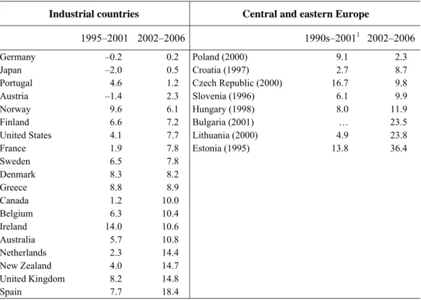
Table 1. Nominal growth of house prices
Four-quarter percentage changes, in national currency units; period averages
Industrial countries Central and eastern Europe
1995–2001 2002–2006 1990s–20011 2002–2006
Germany –0.2 0.2 Poland (2000) 9.1 2.3
Japan –2.0 0.5 Croatia (1997) 2.7 8.7
Portugal 4.6 1.2 Czech Republic (2000) 16.7 9.8
Austria –1.4 2.3 Slovenia (1996) 6.1 9.9
Norway 9.6 6.1 Hungary (1998) 8.0 11.9
Finland 6.6 7.2 Bulgaria (2001) … 23.5
United States 4.1 7.7 Lithuania (2000) 4.9 23.8
France 1.9 7.8 Estonia (1995) 13.8 36.4 Sweden 6.5 7.8 Denmark 8.3 8.2 Greece 8.8 8.9 Canada 1.2 10.0 Belgium 6.3 10.4 Ireland 14.0 10.6 Australia 5.7 10.8 Netherlands 2.3 14.4 New Zealand 4.0 14.7 United Kingdom 8.2 14.8 Spain 7.7 18.4
1 Initial years for country data samples are shown in parentheses.
Source: Authors’ calculations using house price data described in the Appendix.
The picture has changed almost completely since 2002. As income growth accelerated and real interest rates generally continued to fall, nominal house prices in most CEE countries started to grow at double-digit annual rates (Graph 1, upper right-hand panel). In Croatia, the Czech Republic, Hungary and Slovenia, nominal house prices increased by 9–12% per annum between 2002 and 2006, faster than in most industrial countries over this period (Table 1). In Bulgaria, Estonia and Lithuania, nominal house prices have surged by 24–36% per annum on average since 2002, rates unseen in the industrial world. For instance, only Spain has seen average nominal house prices grow by more than 15% per annum over the past five years (Table 1).
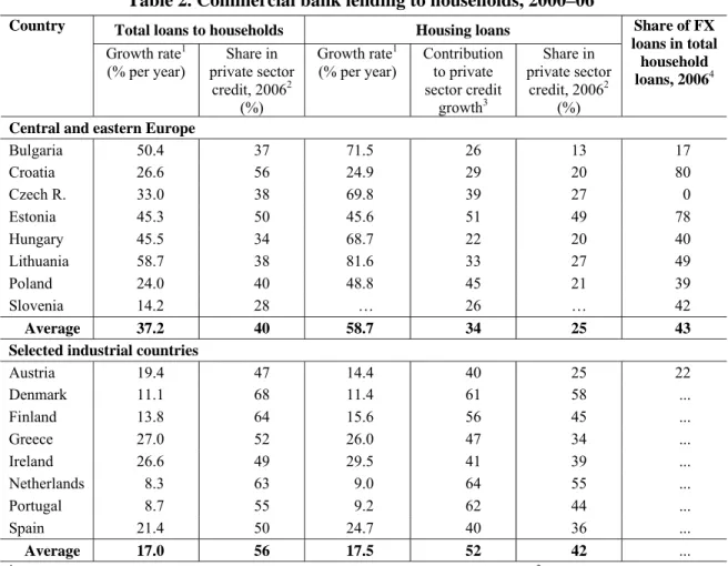
This suggests that, in addition to conventional fundamentals (income and real interest rates), other factors have also played a role in the recent acceleration of house prices. One of these factors has been growth of housing loans, which expanded on average by almost 60% per year between 2000 and 2006, contributing 34% to private sector credit growth in 2005 and 2006 despite a relatively low share in total credit (Table 2).
Graph 1. House prices and macroeconomic fundamentals CEE countries
1995-2001 -15 -5 5 15 25 35 PL HR CZ SI HU BG LT EE
House prices (% p.a.) GDP per capita (% p.a.) dRIR (pct pts, eop) 2002-2006 -15 -5 5 15 25 35 PL HR CZ SI HU BG LT EE
House prices (% p.a.) GDP per capita (% p.a.) dRIR (pct pts, eop)
Selected industrial countries 1995-2001 -15 -5 5 15 PT AT FI DK GR EI NL ES
House prices (% p.a.) GDP per capita (% p.a.) dRIR (pct pts, eop) 2002-2006 -15 -5 5 15 PT AT FI DK GR EI NL ES
House prices GDP per capita Change in real interest rates
Note: For CEE countries, real interest rates represent a weighted average of domestic and foreign currency long-term rates on household loans, deflated by the CPI.
Sources: BIS; IMF; national data; authors’ calculations.
Similar developments, albeit on a smaller scale, have been observed in some industrial countries that are similar to CEE countries in terms of size or catching-up characteristics, including Finland, Greece, Ireland, Portugal and Spain. Real GDP in these countries expanded by 5½% on average during 1995–2001, and by 4½% since 2002 (Graph 1, lower panels). As in CEE, the decline in interest rates was quite pronounced in the second half of the 1990s (–4.6 percentage points on average), as these countries prepared for membership in EMU; and it continued in the 2000s (–1.9 percentage points on average, same as in CEE).
As in CEE, the growth of house prices has accelerated in this group of countries since 2002, to about 9% on average from about 6½% in the second half of the 1990s (Graph 1, lower panels). And as in CEE, rapid credit growth, with housing loans contributing over 50% to total private sector credit growth, may have played an important role in this acceleration. One should note that credit growth in CEE has been to a large extent a transition phenomenon, whereas in industrial countries it has been mainly driven by global factors.
In addition, demographic and labour market factors may have also played a role in housing demand and house prices. Among industrial countries, these factors have promoted housing demand in Ireland, the Netherlands, Scandinavian countries and Spain, especially in the first half of the 2000s. The overall population in CEE is stagnating or declining. However, many CEE countries experienced small baby booms in the 1970s and the early 1980s. As these cohorts approach their prime earning age, they are entering the housing market and providing a strong boost to demand, especially for higher-quality housing. However, some other
institutional and transition-specific factors seem to have played an even greater role in the recent house price take-off in CEE.
Factors specific to housing markets in central and eastern Europe
Until the early 2000s, housing market institutions in most CEE countries were weak and
housing finance almost nonexistent.2 Improvements in the regulatory and institutional
framework necessary for the development of the property market have largely occurred as a result of the EU accession process. In particular, reforms in legislation and judiciary practices that make it easier for creditors to seize real estate collateral removed a key obstacle to the buying and selling of property.
Together with the restructuring of the banking sector and acquisitions of local banks by strategic foreign investors with strong retail expertise, these reforms have spurred the development of housing markets and housing finance (see Mihaljek, 2006). Many banks in CEE started to provide longer-term housing loans; the loan-to-value ratios increased; and
2 Under socialism, most urban housing was provided to workers free of charge by employers or local
authorities. For detailed descriptions of housing market institutions and housing finance in CEE, see OECD (2005) and Palacin and Shelburne (2005).
Table 2. Commercial bank lending to households, 2000–061 Total loans to households Housing loans
Country
Growth rate1
(% per year) private sector Share in
credit, 20062
(%)
Growth rate1
(% per year) Contribution to private
sector credit growth3 Share in private sector credit, 20062 (%) Share of FX loans in total household loans, 20064
Central and eastern Europe
Bulgaria 50.4 37 71.5 26 13 17 Croatia 26.6 56 24.9 29 20 80 Czech R. 33.0 38 69.8 39 27 0 Estonia 45.3 50 45.6 51 49 78 Hungary 45.5 34 68.7 22 20 40 Lithuania 58.7 38 81.6 33 27 49 Poland 24.0 40 48.8 45 21 39 Slovenia 14.2 28 … 26 … 42 Average 37.2 40 58.7 34 25 43
Selected industrial countries
Austria 19.4 47 14.4 40 25 22 Denmark 11.1 68 11.4 61 58 ... Finland 13.8 64 15.6 56 45 ... Greece 27.0 52 26.0 47 34 ... Ireland 26.6 49 29.5 41 39 ... Netherlands 8.3 63 9.0 64 55 ... Portugal 8.7 55 9.2 62 44 ... Spain 21.4 50 24.7 40 36 ... Average 17.0 56 17.5 52 42 ...
1 Annual averages, based on monthly data. CEE data for 2006 are mostly through August. 2 Private sector credit comprises
loans to households and non-financial corporations. 3 Percentage contribution of housing loans to total private sector credit
growth, average for 2005 and 2006. 4 For Croatia, including foreign currency-linked loans.
interest rates started to decline. Although mortgage penetration in CEE remains much lower than in western Europe, and access to mortgage loans is still limited to higher-income households, housing finance is highly competitive, with margins beginning to approach western European levels in some countries.
One can expect the development of housing market institutions and the lifting of credit constraints to be positively correlated with the growth of house prices on both theoretical and empirical grounds. Asset prices, including house prices, tend to rise towards equilibrium levels when markets are deregulated. Empirically, this development was observed in many countries in western Europe in the late 1980s and the early 1990s. For instance, the United Kingdom experienced a major housing boom in the late 1980s during a period of financial liberalisation (see Attanasio and Weber, 1994; and Ortalo-Magné and Rady, 1999).
Another transition-specific factor that has affected house price dynamics in CEE is the
limited supply of new homes. The public sector was for many decades the dominant supplier
of new housing in CEE, especially in the cities. However, it largely withdrew from housing construction during the 1990s due to public expenditure retrenchment. Private construction companies and property developers were slow to fill the resulting void. Even where capacity to build new private homes existed, the supply was constrained because spatial plans were often inadequate. This resulted in a shortage of new housing, so that even in 2005, the supply of new housing in countries such as Bulgaria, Estonia and Lithuania – which, as noted above, recorded the fastest growth of house prices – was far below the supply in western European countries with strong housing markets, such as Denmark, Finland and France, not to mention Ireland and Spain (Graph 2). Against this background of constrained supply, the rapid increase in house prices in some CEE countries should not come as a surprise.
Graph 2. Newly completed dwellings per 1,000 inhabitants
0 5 10 15 20 25 BG LT EE CZ PL SI HU HR IT UK DE NL DK FR FI ES IE 1995 2000 2005
Sources: National statistical offices; UN Economic Commission for Europe.
Improvements in housing quality have been a further factor affecting house price dynamics
in CEE. As recently as 2002, CEE countries scored much lower on measures of housing quality such as average size of dwellings, floor space per occupant, access to piped water, and
fixed baths compared to all but a few industrial countries (Graph 3).3 One would therefore
expect that, once better-quality housing became available on the market, house prices would grow faster on average than in countries where quality of the initial housing stock was higher.
3 The quality of housing measured by these indicators has probably improved since 2002 (the last year for
Rapid growth of house prices in CEE may thus simply reflect a composition effect, where more weight is being given to higher-quality and higher-priced housing.
Graph 3. Indicators of housing quality, 2002
Dwellings with piped water (% ) Dwellings with fixed bath (% ) Dwellings with flush toilet (% )
Source: Czech Statistical Office. 60 70 80 90 100 Po rt ug al L ith ua ni Hu ng ar y Es to ni a Bu lg ar ia Po la nd Ire la nd G re ece Sl ov en ia Fi nl an d C zech R . US De nm ar k Au st ri a S w ed en 60 70 80 90 100 Po rt ug al Es to ni a Li th ua ni a B ulg ar ia Hu ng ar y Po la nd Sl ov en ia G ree ce Ir el an d De nm ar k Cz ec h R. Ge rm an y Au st ri a Fi nl an d US S w ed en 60 70 80 90 100 B ulg ar ia Li th ua ni a Es to ni a Hu ng ar y Po la nd G ree ce Sl ov en ia Cz ec h R. Fi nl an d Ir el an d Ge rm an y De nm ar k Au st ri a US S w ed en
A new factor adding to the rising housing demand in CEE in recent years is increased
external demand. Housing is usually thought of as a non-traded good, but the removal of
restrictions on real estate ownership and increasing labour mobility within the EU are starting to give housing the characteristics of a traded good. The external demand for housing in CEE has three components: the demand for second homes by residents of EU-15 countries (usually retiring baby boomers from Northern Europe); the demand from CEE residents temporarily working abroad (reflecting increased migration and labour “commuting” from eastern to western Europe following EU enlargement in 2004); and investment demand by global real estate companies (which has so far concentrated on commercial real estate, but is increasingly turning to the residential sector).
Anecdotal evidence indicates that external demand for housing in CEE is still relatively small
compared, for instance, with Spain. Nonetheless, it plays an important role in house price
dynamics because it affects sellers’ expectations. If the supply of land for construction is limited due to slow adjustment of zoning regulations, external demand will lead to an increase in land prices. This increase can spill over to house prices for local residents, as landowners are unwilling to sell land at lower prices for local housing projects if they can obtain a higher price from foreign buyers (see Mihaljek, 2005).
Like prices of other assets, house prices can occasionally be disconnected from underlying
fundamentals. In the case of CEE, one reason for house price misalignment could be highly
distorted relative prices at the beginning of the transition, ie, the initial undershooting. The price of housing relative to the price of other consumer durables (or the level of rents relative to the price of other consumer services) was severely distorted under socialism. This distortion was not corrected immediately after the move from plan to market because the bulk of the housing stock was privatised at artificially low (non-market) clearing prices. This has led to very low turnover in the property market, given that the proportion of privately-owned
and owner-occupied housing in CEE is very high.4 Another reason for the low turnover was
the relative homogeneity of existing housing stock. As most housing was built in apartment
4 Private individuals in CEE own on average 80–95% of the housing stock, and the ratio of owner-occupied
housing in many countries exceeds 90% (OECD, 2005). In western Europe, the share of housing owned by private individuals ranges from about 60% in Austria and Sweden to 90–95% in Belgium, Greece, Spain and Portugal, while the share of owner-occupied housing ranges from 38% in Germany to 80% in Ireland.
blocks after the Second World War, there was not much opportunity for moving up the housing “ladder” as is common in western European countries.
As housing privatisation had come to a close and institutional, regulatory and housing finance reforms were being implemented, the initially distorted relative prices started to move towards equilibrium. One piece of anecdotal evidence of the magnitude of this change – and, hence, the extent of initial undershooting – is provided by the change in the price of an apartment in a typical block of CEE flats built in the 1970s relative to the price of a middle-class passenger car produced in western Europe, such as a Volkswagen Golf. In the early 1990s, this relative price was roughly 1:1. By 2006, the same unrenovated apartment was roughly four times more expensive than the VW Golf. In other words, even without any commensurate change in underlying fundamentals, the fourfold increase in the relative price of housing over the past 15 years would have been consistent with the correction of initial undershooting.
ECONOMIC AND ECONOMETRIC APPROACH
This section first describes data issues, which are of paramount importance for explaining the empirical results of this paper; then elaborates on the regressions that are used to estimate the determinants of house prices; and finally describes the econometric methodology used to obtain these estimates.
Data issues
Our dataset comprises quarterly data covering 27 countries, grouped into two main panels:
developed non-transition OECD countries and CEE transition economies.5 Based on the size
of the economy and growth rates of GDP, the OECD panel is further split into three
sub-panels: large, small and catching-up OECD countries.6 Analogously, the CEE panel, which
consists of eight transition economies, was split into CEE slow (Croatia, the Czech Republic,
Hungary, Poland and Slovenia) and CEE fast (Bulgaria, Estonia and Lithuania). The dataset is
unbalanced, as the lengths of the individual data series depend largely on data availability. The sample begins between 1975 and 1994 for the OECD countries, and between 1993 and 1998 for the transition economies, and ends in 2005.
In addition, we faced two major constraints. First, given that we cover a large number of countries in an attempt to compare the determinants of house prices in developed and catching-up economies, it was very difficult to obtain a comprehensive and comparable dataset for some of these variables. Second, given the low number of observations for transition economies, our model could include only a limited set of explanatory variables in a dynamic panel context.
The data that are of greatest interest for this study, and took the most time to collect, are those on house prices in CEE countries. When comparing different measures of house prices, one faces severe limitations because housing is very heterogeneous. Data from national sources refer to different types of residential property (new vs existing housing; apartments in different types of buildings; single vs multiple-family houses), so large differences in growth
5 CEE countries that are members of the OECD are included only in the transition economies sample.
6 The large OECD sample comprises France, Germany, Japan, the United Kingdom and the United States.
The small OECD sample comprises Austria, Belgium, Finland, Greece, Ireland, the Netherlands, Portugal and Spain from the euro area; plus Denmark, Norway, Sweden, Australia, Canada and New Zealand. The catching-up sample includes Greece, Ireland, Portugal and Spain.
rates of house prices for the same city, region or country are not unusual. These differences are even greater if the data from commercial sources (eg real estate companies) are considered, which is often necessary given the lack or inadequate coverage of the official data.
We collected the house price data from the BIS Data Bank, central banks (see eg Kiss and Vadas, 2005), and, in some cases, statistical offices. The underlying data refer either directly to prices per square metre of residential housing sold (with coverage by cities/regions and type of housing varying from country to country), or to the house price indices that are linked to the prices per square metre or to the average prices of apartments or houses. For the OECD countries, house price data were mostly obtained from the BIS Data Bank and Datastream. In regressions, all house prices are expressed in real terms, ie, as nominal prices deflated by the country’s CPI.
Other data represent standard macroeconomic variables and, together with the house price series, are described in detail in the Appendix.
Despite its obvious importance, this paper could not address the issue of equilibrium or “excessive” growth of house prices in CEE. Aside from methodological issues (see Maeso-Fernandez et al, 2005), the main problem was the lack of adequate data. In particular, the out-of-sample panel approach – ie using the estimation results obtained for the OECD countries to derive misalignments for CEE countries (as was done, for instance, in the study of equilibrium credit growth in CEE by Egert et al, 2007) – was not feasible. Among small OECD countries, which could be taken as a natural long-term benchmark for CEE, only two
countries – Finland and Ireland – publish data on house price levels, measured in euros per
square metre, that are available throughout the sample period. For instance, Australia, Austria, Belgium, Canada, Denmark, Germany, Greece, the Netherlands, Portugal and Sweden publish only time series for house price indices, and not the data on levels of house prices per square
metre at a quarterly or monthly frequency.
The empirical model
Our baseline specification tries to explain real house prices (phouse), defined as nominal house
prices deflated by the CPI, with real income and real interest rates (equation 4). We used three different specifications of real income: GDP per capita converted to euros using PPP rates (capita PPP); GDP per capita at constant prices (capita const); and cumulated real GDP
growth (gdpr). The results did not differ significantly across these specifications, so we report
only the estimates using per capita income. Real interest rates (rir) are defined in an ex-post
sense, as nominal interest rates deflated by annualised inflation rates (it/(pt− pt−4). In this simple specification, changes in real house prices are expected to be positively correlated with changes in real income and negatively correlated with changes in real interest rates:
) ,
( + −
= f capita rir
phouse (4)
We also experimented with nominal interest rates as an explanatory variable. Sutton (2002) and Tsatsaronis and Zhu (2004) show that nominal interest rates perform better than real interest rates in explaining house prices, given that banks typically make the decision to grant a housing loan based on the ratio of debt servicing costs to income, which depends on the nominal and not the real rate. However, the nominal interest rate elasticities that we obtained were either positive or statistically insignificant.
The interest rates in equation (4) are initially those on domestic currency loans to the private sector. In CEE, an important share of lending is denominated in foreign currencies. Therefore,
we use a weighted average of real interest rates on domestic and foreign currency (euro)
housing loans (rir mix), which is perhaps the most precise measure of the cost of housing
loans from the available time series data (equation 4a). )
,
( + −
= f capita rirmix
phouse (4a)
To this baseline specification we add, one by one, four complementary control variables. These are the equity price index (stock mkt), to capture the influence of equity prices on house
prices (via wealth effects induced by changes in equity prices, or as an investment alternative to real estate) (equation 5); and three variables relating to the labour market and demographic
factors – the unemployment rate (unemp) (equation 6), the share of the working-age
population in total population (pop) (equation 7), and the share of the labour force in total
population (labforc) (equation 8):
) ,
,
( + − +
= f capita rir stockmkt
phouse (5)
) ,
,
( + − −
= f capita rir unemp
phouse (6)
) , ,
( + − +
= f capita rir pop
phouse (7)
) ,
,
( + − +
= f capita rir labforc
phouse (8)
We also used credit as a percentage of GDP as one of the control variables. However, since per capita income and housing credit are strongly correlated, multicollinearity arises in empirical estimates. To tackle this problem, we estimate separately an equation excluding per
capita GDP and including only housing loans (credit hsg) (equation 9)
) ,
( − +
= f rir credithsg
phouse (9)
Collecting the data that capture the impact of transition-specific factors presented considerable problems. The impact of improved quality of housing on house prices is a tricky issue because statistical offices in CEE – as in many western European countries – do not compile quality adjusted indicators of house prices, and because it is difficult to find explanatory variables that capture improvements in housing quality. One indirect measure of changes in housing quality that can be constructed from the available data is the real value of residential construction per square metre of newly constructed dwellings. This indicator is obtained as the value of residential construction per average area of new dwellings (excluding land prices and adjusted for changes in average area) deflated by the construction cost index. While the time span is rather short, Graph 4 suggests that, measured by this indicator, housing quality increased in most, though not all, CEE economies between 2000 and 2004. Moreover, changes in real house prices during 2000–04 were generally closely correlated with this indicator of housing quality. The exceptions were countries where due to capacity constraints (in particular shortage of construction workers) real construction costs increased faster than real house prices (eg Croatia, Hungary, Estonia, Lithuania and Spain).
Graph 4. House prices and real value of newly constructed housing, 2000–04 86 93 94 103 12 1 12 4 12 5 16 4 16 7 251 26 0 384 387 94 117 12 5 104 13 7 114 117 145 111 13 5 17 3 185 25 3 0 100 200 300 400 PT FR SE SI BG DK FI CZ HR HU LT ES EE
Increase in value of residential construction per average area (in m2) of new dwellings, deflated by construction cost index, 2000=100 Increase in average house prices, deflated by CPI, 2000=100
Sources: National statistical offices; authors’ calculations.
As the underlying data series used in constructing this index were incomplete, we used real
wages in the whole economy (rwage) as a broad proxy for changes in housing quality. From
an econometric perspective, the possibility of a strong correlation between GDP per capita and real wages is an important issue – real wages can be viewed as an alternative measure of per capita income. Conversely, changes in GDP per capita could also include information about changes in housing quality. As a result, when using real wages as a proxy for housing quality, we exclude GDP per capita from our regressions.
Moreover, real wage growth also reflects the catching-up process resulting from differential productivity growth in tradable and non-tradable industries (the Balassa-Samuelson effect). In this interpretation, rising wages are a manifestation of the same catching-up phenomenon that leads to improvements in housing quality. Furthermore, real wages – to the extent reflected in wage developments in the construction sector – are an important component of construction costs. Consequently, real wage growth are associated with an increase in house prices.
) ,
( − −/+
= f rir rwage
phouse (10)
Our search for variables describing external demand for housing was unsuccessful. CEE countries do not publish data on house sales to non-residents, so we tried to proxy the effects of external demand on house prices with monetary aggregates (M2 or M3), since house sales to non-residents are typically settled in cash and should therefore be reflected in bank deposits. However, the size of coefficients we obtained was very small and there was evidence of multicollinearity between monetary aggregates and per capita income.
Regarding institutional factors, the European Bank for Reconstruction and Development (EBRD) compiles a number of transition indicators that are potentially relevant for measuring the pace of development of housing markets and housing finance. These include indicators of
banking reform and interest rate liberalisation (bkg reform) (equation 11a), and indicators of
security markets and non-bank financial institutions’ reform (nbfi reform) (equation 11b):
) ,
,
( + − +
= f capita rir bkgreform
phouse (11a)
) ,
,
( + − +
= f capita rir nbfireform
phouse (11b)
The first step was to check whether the series under study are stationary in levels. We used four panel unit root tests: the Levin, Lin and Chu (2002), the Breitung (2000), the Hadri (2000) and the Im-Pesaran-Shin (2003) tests. The first three tests assume common unit roots across panel members, whereas the Im-Pesaran-Shin test allows for cross-country heterogeneity. The Hadri test considers the null of no unit root against the alternative hypothesis of a unit root. The remaining tests take the null of a unit root against the alternative hypothesis of no unit root. The tests were carried out for level, first-differenced and second-differenced data. The results (not reported because of space constraints) usually indicated that the series were I(1) processes. Some of the tests showed that a few series were I(0) or I(2), but given no overwhelming evidence that they were really stationary in levels or in second differences, we assumed that they were stationary in first differences.
The main econometric technique used in this paper is the panel dynamic OLS, which is the mean group of individual DOLS estimates. The existence of long-term relationships that connect house prices to a set of explanatory variables is checked by using the error-correction terms derived from the error-correction specification of the panel DOLS model. If the error correction term (ρ) in equation 12 has a negative sign and is statistically significant, then one can establish a cointegrating vector:
t i n h t h i h i n h t i h i t i i i t i Y X X Y , 1 , , , 1 1 , , 1 , , =α +ρ ( − β )+ γ ∆ +ε ∆
∑
∑
= = − − (12)The coefficients of the long-term relationships are obtained using panel DOLS estimations,
which can be written for panel member i as follows:
t i n h k k j j t i j i n h t i h i i t i i i X X Y , 1 , , 1 , , , 2 , 1 , ε γ β α + + ∆ + =
∑
∑ ∑
= =− − = (13)where ki,1 and ki,2 denote, respectively, leads and lags; and the cointegrating vector β'
contains the long-term coefficients of the explanatory variables (with h=1,...,n) for each
panel member i. The Schwarz information criterion is used to determine the optimal lag
structure. The panel DOLS accounts for the endogeneity of the regressors and serial correlation in the residuals in the simple OLS setting, by incorporating leads and lags of the regressors in first differences (Kao and Chiang, 2000). This is a very useful feature as some of the explanatory variables (such as housing loans) may be endogenous (see eg Hofmann, 2001). The panel DOLS also allows for cross-country heterogeneity in both short-run and long-run coefficients.
ESTIMATION RESULTS
The estimates of long-term relationships between changes in real house prices and their determinants are presented in Tables 3–5. The tables also show the estimates of
error-correction terms (ECT) from the corresponding error-correction specifications (equation 12)
of the panel DOLS models. All error-correction terms reported fulfil the double criterion of negative sign and statistical significance necessary to establish a long-term cointegrating relationship between real house prices and the selected explanatory variables.
A striking feature of the results is the large difference in the size of the error-correction
terms for the OECD countries on the one hand, and CEE countries on the other. While the
error-correction terms range from –0.05 to –0.11 for the OECD panel (Table 3A), for the CEE panel they range from –0.15 to –0.33 (Table 3B). This indicates a much higher speed of adjustment to equilibrium growth of house prices in the case of CEE transition economies than in the case of OECD countries.
GDP per capita is highly significant and has the expected positive sign in virtually all
regressions, indicating that changes in income are strongly positively related to changes in house prices. Another important result is that income elasticities of house prices are much higher in transition countries (Table 3B) than in OECD economies (Table 3A). Among OECD countries, income elasticities of house prices are higher for the catching-up countries (up to 1.0, Table 4B) than the small countries (up to 0.8, Table 4A). Similarly, among transition countries, income elasticities are higher for CEE fast (up to 2.0, Table 5B) than CEE slow (up
to 0.8, Table 5A). The highest income elasticities of house prices thus belong to the group of
countries with the fastest growth of per capita GDP (CEE fast), and the lowest to the group
with the slowest GDP growth (small OECD).
Real interest rate coefficients in most cases have the expected negative sign and are
statistically significant, indicating that lowering of real interest rates is associated with rising real house prices. As with real income, real interest rate elasticities of house prices are much higher in transition economies (up to –0.05, Table 3B) than in OECD countries (up to –0.02, Table 3A). In other words, for the same decline in real interest rates, house prices in central and eastern Europe have tended to increase up to 2½ times faster than in OECD countries. Given that the decline in real interest rates in CEE has been much more pronounced than in OECD countries, the observed faster growth of house prices in CEE should therefore not come as a surprise.
Credit (measured by changes in the ratio of private sector credit to GDP in OECD countries,
and by the ratio of housing credit to GDP in transition economies) has a strong positive relationship to house prices, both in OECD countries and in transition economies. Interestingly, estimated credit elasticities are higher for OECD countries than for transition economies, both in the large sample (Table 3A vs 3B) and in sub-samples. For instance, in the catching-up OECD countries the estimated elasticity of house prices with respect to credit is
0.96 (Table 4B); in small OECD countries 0.76 (Table 4A); and in CEE fast 0.41 (Table 5B).
In other words, house prices respond roughly two times more strongly to changes in credit in
OECD countries than in CEE fast economies. It is also interesting to note that the explanatory
power of regressions including credit growth is not significantly different from those including per capita income, which indicates how correlated these two variables are.
Confirming the findings of earlier studies, coefficient estimates for population, labour force
and unemployment for the OECD countries are all significant and have the expected signs
(Tables 3A, 4A and 4B). In CEE slow, a clear and robust relationship exists only between
population and house prices (Table 5A). In CEE fast, the predicted relationship is confirmed
for labour force and unemployment (Table 5B). One can notice that the size of estimated coefficients is higher in CEE than in OECD countries. For instance, the labour force elasticity in CEE fast is 8.4, compared with 1.1 in small OECD countries; the unemployment elasticity
is –0.9 in CEE fast compared with –0.2 in catching-up OECD; and the population growth
elasticity is 17.0 in CEE slow, compared with 5.0 in small OECD.
House prices in OECD countries are negatively correlated with equity prices, indicating the
prevalence of substitution effects. For instance, the coefficient estimate in the OECD catching-up sample is –0.16 (Table 4B). In CEE, changes in equity prices are, by contrast,
positively correlated with changes in house prices, indicating possible wealth effects. For
instance, in CEE fast, a 1 percentage point increase in equity prices is associated with an
increase in house prices of 0.16 percentage points (Table 5B). Note, however, that this result is a bit surprising, given that only a small proportion of the population in CEE holds equities.
Estimation results – long-term relationships
Dependent variable: change in real house prices Table 3A: All OECD countries
Eq(4) Eq(9) Eq(5) Eq(6) Eq(7) Eq(8) Eq(10)
capita PPP 0.434** 0.590** 0.467** 0.507** 0.459** rir –0.003** –0.015** –0.005** 0.007 –0.005** –0.003** –0.002** credit 0.617** stock mkt –0.023** unemp –0.197** pop 4.456** labforc 1.065** rwage 0.009** ECT –0.073** –0.046** –0.077** –0.106** –0.099** –0.084** –0.057** R2 0.68 0.69 0.76 0.80 0.80 0.75 0.78
Note: ** indicates statistical significance at the 5% significance level. ECT is the error correction term.
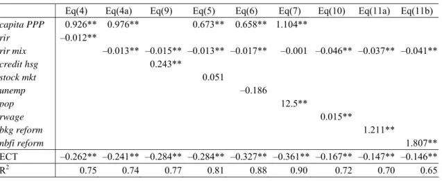
Table 3B: All CEE countries
Eq(4) Eq(4a) Eq(9) Eq(5) Eq(6) Eq(7) Eq(10) Eq(11a) Eq(11b)
capita PPP 0.926** 0.976** 0.673** 0.658** 1.104** rir –0.012** rir mix –0.013** –0.015** –0.013** –0.017** –0.001 –0.046** –0.037** –0.041** credit hsg 0.243** stock mkt 0.051 unemp –0.186 pop 12.5** rwage 0.015** bkg reform 1.211** nbfi reform 1.807** ECT –0.262** –0.241** –0.284** –0.284** –0.327** –0.361** –0.167** –0.147** –0.146** R2 0.75 0.74 0.77 0.81 0.88 0.90 0.72 0.70 0.65
Note: ** indicates statistical significance at the 5% significance level. ECT is the error correction term.
Table 4A: Small OECD countries1
Eq(4) Eq(9) Eq(5) Eq(6) Eq(7) Eq(8) Eq(10)
capita PPP 0.553** 0.751** 0.591** 0.675** 0.606** rir –0.005** –0.019** –0.006** 0.006 –0.002** –0.006** –0.009** credit 0.756** stock mkt –0.031** unemp –0.211** pop 5.011** labforc 1.113** rwage 0.011** ECT –0.091** –0.053** –0.099** –0.133** –0.126** –0.106** –0.069** R2 0.71 0.71 0.81 0.85 0.84 0.78 0.80
1 Australia, Austria, Belgium, Canada, Denmark, Finland, Greece, Ireland,
the Netherlands, New Zealand, Norway, Portugal, Spain and Sweden.
Note: ** indicates statistical significance at the 5% significance level. ECT is the error correction term.
Table 4B: Catching-up OECD countries1
Eq(4) Eq(9) Eq(5) Eq(6) Eq(7) Eq(8) Eq(10)
capita PPP 0.673** 1.004** 0.566** 0.847** 0.524** rir –0.007** 0.000 –0.003** –0.003** –0.001 0.000** –0.015** credit 0.960** stock mkt –0.157** Unemp –0.213** Pop 5.544** Labforc 1.192** Rwage 0.009** ECT –0.159** –0.107** –0.175** –0.220** –0.181** –0.165** –0.094** R2 0.80 0.74 0.82 0.91 0.88 0.81 0.89
1 Greece, Ireland, Portugal and Spain.
Note: ** indicates statistical significance at the 5% significance level. ECT is the error correction term.
Table 5A: CEE slow countries1
Eq(4a) Eq(9) Eq(5) Eq(6) Eq(7) Eq(8) Eq(10) Eq(11a) Eq(11b)
capita PPP 0.484** 0.469** 0.454** 0.812** 0.578** rir mix –0.001 –0.001 0.005 –0.012** 0.010 –0.007** 0.000 –0.010** 0.007 credit hsg 0.144** stock mkt 0.019** unemp 0.226** pop 17.01** labforc –1.166 rwage 0.006** bkg reform 0.275** nbfi reform 0.625** ECT –0.251** –0.292** –0.300** –0.282** –0.413** –0.360** –0.232** –0.170* –0.247** R2 0.64 0.65 0.82 0.826 0.86 0.84 0.59 0.57 0.48
1 Croatia, the Czech Republic, Hungary, Poland and Slovenia.
Note: * and ** indicate statistical significance at the 10% and 5% significance levels, respectively. ECT is the error correction term.
Table 5B: CEE fast countries1
Eq(4a) Eq(9) Eq(5) Eq(6) Eq(7) Eq(8) Eq(10) Eq(11a) Eq(11b)
capita PPP 1.796** 1.036** 0.997** 1.268** 1.964** rir mix –0.035** –0.037** –0.043** –0.026** 0.016**– –0.003 –0.122** –0.074** –0.105** credit hsg 0.408** stock mkt 0.155** unemp –0.873** pop 14.477 labforc 8.355** rwage 0.031** bkg reform 3.193** nbfi reform 3.383** ECT –0.225** –0.272** –0.258** –0.403** –0.271** –0.059* –0.116* –0.012 R2 0.91 0.97 0.96 0.98 0.98 0.94 0.87 0.88
1 Bulgaria, Lithuania and Estonia.
Note: * and ** indicate statistical significance at the 10% and 5% significance levels, respectively. ECT is the error correction term.
Real wages, used as a broad proxy for housing quality, are positively correlated with real
house prices. This result holds for all country sub-groups. The estimated real wage elasticity
of house prices is highest in CEE fast (0.031; Table 5B), followed by OECD small (0.011;
Table 4A) and catching-up 4 (0.009; Table 4B). To the extent that real wages, as an important
component of construction costs, adequately reflect improvements in housing quality, these results support the view that better housing quality had a stronger impact on house prices in those countries where housing quality was initially lower.
EBRD transition indicators, used as proxies for the development of the housing market and
housing finance institutions, perform fairly well. An increase in the banking reform
indicator by one unit adds as much as 3.2 percentage points to the real growth of house prices in CEE fast in the long run (Table 5B) and 0.3 percentage points in CEE slow (Table 5A). The
improvement in the non-bank financial institutions’ indicator has an even stronger effect,
adding 3.4 percentage points to the growth of real house prices in CEE fast and 0.6 points in
CEE slow. These results provide support to the view that the development of housing markets
and housing finance institutions has had a major impact on the dynamics of house prices in central and eastern Europe.7
CONCLUSIONS
This paper studied the determinants of house price dynamics in eight transition economies of central and eastern Europe and 19 OECD countries using panel DOLS techniques. We analysed the role played in house price dynamics by the traditional fundamentals such as real income, real interest rates and demographic factors; and the importance of some transition-specific factors, such as improvements in housing quality and in housing market institutions and housing finance. We also analysed how these various factors affected house price dynamics across different groups of OECD and transition economies.
Notwithstanding serious problems regarding the quality of data on house prices and their determinants, one can on the whole conclude that the fundamentals have played an important role in explaining house prices in both CEE and OECD countries. We established a strong positive relationship between per capita GDP and house prices. We also established robust relationships between real interest rates and house prices, as well as between housing (or private sector) credit and house prices, in both CEE and OECD countries. House prices in central and eastern Europe have tended to increase twice as fast for an equivalent drop in real interest rates than house prices in OECD countries. On the other hand, house prices in OECD countries seem to respond roughly two times more strongly to credit growth compared with CEE economies. The observed rapid credit growth in central and eastern Europe may therefore have smaller impact on the growth of house prices than is usually extrapolated from relationships obtained for the OECD countries.
Demographic factors and labour market developments also play an important role in house price dynamics. They seem to affect house prices more strongly in central and eastern Europe than in OECD countries.
Finding appropriate indicators to assess the impact of transition-specific factors on house price dynamics in CEE proved to be challenging. As a broad proxy for improvements in housing quality we used the growth of real wages. We could establish that house prices responded more strongly to increases in real wages in those countries where housing quality was initially lower.
7 As in the case of credit and real wages, regression estimates with EBRD indicators exclude GDP per capita
Similarly, the development of housing markets and housing finance institutions (proxied by EBRD indicators of bank and non-bank financial institutions’ reform) seems to have a fairly strong impact on real house price dynamics in central and eastern Europe. Countries that have implemented greater and faster improvements in these institutions have also tended to experience faster growth of house prices.
Our dataset did not allow us to investigate fully all the economically interesting issues related to house price developments in central and eastern Europe. In particular, because of the lack of reliable data on levels of house prices in OECD countries (measured in euros per square metre of residential housing), we were not in a position to assess the possible degree of house price misalignments in CEE countries vis-à-vis comparable OECD economies.
Nevertheless, we could shed some light on the question of adjustment from initial undershooting by looking at the estimates of coefficients on per capita GDP. These estimates were very high (up to 2.0) for those CEE countries that experienced the fastest growth of house prices (Bulgaria, Estonia and Lithuania), as well as for the catching-up OECD countries (Greece, Ireland, Portugal and Spain) (up to 1.0). Separately, we obtained much higher error correction terms for CEE countries, indicating much faster adjustment to equilibrium growth of house prices in CEE.
These results might also partly reflect correction from initial undervaluation of house prices in CEE countries, given that they were highly distorted relative to prices of other consumer durables at the start of the transition. But they might also indicate potential overshooting. Nevertheless, if house prices in these countries had been completely disconnected from fundamentals, we should have established the absence of any statistical relationship between house prices and GDP per capita and other fundamentals.
Appendix
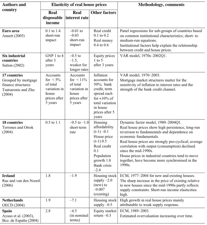
Table A1. Selected recent empirical studies on the determinants of house prices Elasticity of real house prices
Authors and country Real disposable income Real interest rate Other factors Methodology, comments Euro area Annett (2005) 0.1 to 1.4 short-run impact –0.01 to –0.03 short-run impact Real credit 0.1 to 0.2 Real money 0.4 to 0.6
Panel regressions for sub-groups of countries based on common institutional characteristics; short- to medium-run equations.
Institutional factors help explain the relationship between credit and house prices.
Six industrial countries Sutton (2002) GNP 1 to 4 after 3 years –0.5 to –1.5, weaker for longer rates Equity prices 1 to 5 after 3 years VAR model, 1970s–2002Q1. 17 countries Grouped by mortgage finance structures Tsatsaronis and Zhu (2004) Accounts for < 5% of total variation in house prices after 5 years Accounts for < 11% of total variation in house prices after 5 years Inflation accounts for 50%; bank credit, term spread each for ≈10% of total variation in house prices after 5 years VAR model, 1970–2003.
Mortgage market structures matter for the sensitivity of inflation to interest rates and the strength of the bank credit channel.
18 countries
Terrones and Otrok (2004) 0.5 to 1.1 –0.5 to –1.0 short-term rate Housing affordability (t-1) –0.1 House price (t-1) 0.5 Real credit 0.1 Population growth 1.8 Bank crisis –2.4
Dynamic factor model, 1980–2004Q1.
Real house prices show high persistence, long-run reversion to fundamentals and dependence on economic fundamentals.
Real house prices are strongly pro-cyclical; average correlation with output (consumption) declined since the mid-1990s.
House prices in industrial countries tend to move together, have become more synchronised in the 1990s.
Ireland
Rae and van den Noord (2006) 1.8 –1.9 Housing stock supply –2.0 (new) to –0.007 (existing)
ECM, 1977–2004 for new and existing houses. The sharp increase in the price of existing relative to new houses since the mid-1990s partly reflects supply constraints. Short-run income elasticities high.
Netherlands
OECD (2004)
1.9 –7.1 Housing stock
supply –0.5 High growth in real house prices mainly attributable to weak supply response.
Spain Ayuso et al. (2003), Bco. de España (2004) 2.8 –4.5 (in nominal terms) Equity market
return –0.3 ECM, 1989–2003. Estimated overvaluation increasing over time. Source: Adapted from Girouard et al (2006), pp 11–15.
Box 1
House prices in CEE and OECD economies
House prices are considerably lower in central and eastern Europe than in western Europe. Real estate company data collected by the European Council of Real Estate Professions indicate that in 2005 average house prices in euros per square metre in Bulgaria, Estonia and Lithuania were about four times lower than those in Italy, Finland, the Netherlands and Sweden; and six to seven times lower than those in Spain and France (Graph A1).
Graph A1
Ave rage house price s, 2005 In EUR/ m2 77 0 89 0 1,11 0 1, 20 0 1, 27 0 1, 31 0 1, 50 0 1, 52 0 1, 60 0 1, 90 0 2, 00 0 2,80 0 2, 88 0 2, 88 0 2, 90 0 3, 40 0 4,04 0 4, 30 0 5,00 0 5,56 0 0 1,000 2,000 3,000 4,000 5,000 6,000 Bu lg ar ia L ithua ni a H unga ry Po la nd E st oni a C ze ch R ep. Ge rm an y Be lg iu m Au st ri a Cro at ia Sl ove ni a N eth er la nd s Sw ed en It al y Fi nl an d No rw ay De nm ar k Ir el an d Sp ai n Fr an ce Capital city Second largest city
Source: European Council of Real Estate Professions.
However, when house prices are compared across some capital cities, these differences narrow significantly and sometimes even disappear. In 2005, a square metre of housing in Budapest, Prague or Warsaw cost just 20–30% less than in Berlin, Brussels or Vienna; in Ljubljana and Zagreb, average house prices were the same or higher than in the latter three western capitals (Graph A1). This is the result of increasing concentration of economic activity, especially the booming service industries, in urban areas in CEE countries. Urban land prices – and, by extension, urban house prices – thus often increase much faster than house prices in the countryside.
Data description8
House prices OECD economies
AU: residential property prices, existing dwellings, 8 cities, per dwelling nsa, weighted average of eight state
capitals: Sydney, Melbourne, Brisbane, Adelaide, Perth, Hobart, Darwin, Canberra; house price indices, established houses. BIS code: Q:VSKA:AU:25, 86:q3-06:q1
AT: residential property prices, all dwellings, Vienna, per square metre, quarterly average, nsa; index, 2000 =
100; price per square metre of usable space; new and existing flats and single-family houses; OeNB, original source: Austria Real Estate Exchange, Vienna University of Technology, Institute for Urban and Regional Research. BIS code: Q:VSJA:AT:40, 86:q3-05:q4
BE: all dwellings, whole country, per dwelling, monthly average, nsa; index, 1988 = 100; existing and new
dwellings. BIS code: Q:VSJA:BE:05, 88:q1-05:q4
CA: national monthly residential average price, actual Canadian real estate association, existing dwellings. BIS
code: M:VSKA:CA:05, monthly, 80:q1-06:q2
DE: 2000 = 100; units and prices weighted with population of each city in 2000; good quality new flats in 100
cities; calculated by the central bank BIS code: A:VSLA:DE:54, 75-05
DK: all dwellings, Denmark, per dwelling, nsa; index, 1980 = 100; cash price of new and existing one-family
dwellings sold. Price measure: purchase price at cash value in percentage of officially appraised cash value in 1992, ordinary free trade, quarterly. BIS index: Q:VSJA:DK:05, 71:q1 – 05:q4
FR: Banque de France,80:q4-05:q1
FI: residential property prices, urban areas block of flats and terraced houses, existing dwellings, price euro per
square metre. Datastream code: FNHOUSEAA, 83:q1-05:q4
GR: all dwellings, urban Greece excluding Athens, per dwelling, nsa; covers 13–17 cities with more than 10,000
inhabitants; Bank of Greece. BIS code: Q:VSJA:GR:55, 94:q1-06:q1
IE: new residential property, average of observations through period, price per house, annual. BIS code:
A:VSLA:IE:06A, 71-05
JP: average mansion price per household-capital area, monthly. Datastream code: JPTOMAAPA, 77:q1 – 06:q2
NL: MEES PIERSON real estate price index, monthly. Datastream code: NLMHREPI, 70:q1 – 06:q2
PT: residential property prices, all houses, urban areas, per square metre, nsa-disc. Index, 1988 Jan = 100,
average supply values per square metre usable areas covers old and new houses in over 30 distinct locations in medium/large towns of Portugal mainland, monthly. BIS code: M:VSJA:PT:91, 88:q1-05:q2
ES: For 1987–1998, average price per square metre for appraised housing in municipalities > 500,000
inhabitants, weighted by 1991 population; Banco de Espana estimates based on Ministerio de Fomento and INE; BIS code: q:vska:es:93. For 1999–2004, average price per square metre for appraised housing in municipalities > 500,000 inhabitants, weighted by 1991 population; Banco de Espana estimates based on Ministerio de Fomento and INE; BIS code: Q:VSKA:ES:32, 87:q1-04:q4
NO: residential property prices, existing dwellings (Norway) per dwelling, nsa index, 2000 = 100. Units
registered, purchase price of the building. BIS code: Q:VSKA:NO:05, 91:q1-06:q1
SE: residential property prices, all owner-occupied dwellings, Sweden, per dwelling, nsa; index; based on the
legal registrations; adjusted for rateable values and weighted to represent the actual stock of houses; covers existing stock of one- and two-dwelling buildings; price index of owner-occupied new and existing dwellings for permanent use; Statistics Sweden. BIS code: Q:VSJA:SE:05, 87:q1-05:q4
NZ: residential property prices, all houses, big cities, per house, q-all nsa-disc. BIS code: Q:VSJA:NZ:91,
70:q1-06:q1
UK: nationwide house price index of all properties. Datastream code: UKNWALLP, 70:q1-06:q1
US: median price of new one-family houses sold during month. Datastream code: USHOUSEM, 70:q1-06:q1
CEE economies
BG: National Statistical Institute, end of period, Bulgarian lev per square metre, statistical survey based on real
contracts for existing flats in regional centres, National Statistical Institute, average quarter market prices of dwellings. BIS code: Q:VSKA:BG:24, 00:q1-06:q2
8 Yearly data are linearly interpolated to quarterly frequency. Monthly data are transformed to quarterly
CZ: Czech Statistical Office, average of observations through period. Index 2000 = 100, index of residential property prices from data compiled from tax returns. Covers classic building site or land, but not farm land, free or developed. BIS code: Q:VSWA:CZ:01, 99:q1- 06:q2
EE: for 1993–1996, Bank of Estonia. For 1997–2001, Statistical Office, purchase-sale contracts of movable
assets. Since 2002, purchase-sale contracts of real estate, dwellings in satisfactory condition. Prices of 2-room flats, average purchase-sale price per square metre of dwellings of satisfactory condition, Estonia kroon per square metre. BIS code: Q:VSKA:EE:44, 93:q1–2006:q1
HU: data used in Kiss and Vadas (2005): Central Statistical Office, weighted average (by number of
transactions) prices of purchase-sale contracts registered at the regional Land Registry Offices, HUF per square metre, yearly data (see Kiss and Vadas for the interpolation to quarterly frequency). 97:q1-05:q2
HR: hedonic price index of residential property (HICN), average transactions prices, semi-annual data;
calculated by Croatian National Bank (see HNB Bulletin, December 2006); 1997_h1=100, 97:h1-06:h1
LT: State register, quarterly data, 98:q4- 06:q2
PL: Central Statistical Office, price of a square metre of usable floor space of a residential building, established
on the basis of outlays incurred by investors other than individual in construction of new residential buildings, excluding one-dwelling buildings
SI: Bank of Slovenia, 2-room flat in Ljubljana, SIT per square metre, 95:q2-06:q2
GDP
GDP per capita, AMECO, yearly data, full coverage
GDP at constant market prices per head of population, at 2000 market prices, in national currency (code: 1.1.0.0.RVGDP)
GDP at current market prices per head of population, at PPS (code: 1.0.212.0.HVGDP) Real cumulated GDP growth: IFS, quarterly
Nominal GDP, AMECO, 1.0.0.0.UVGD, yearly data, full coverage
Interest rates OECD economies
Bank lending rates (IFS line 60p); where not available, long-term government bond yields (IFS line 61) CEE economies
Bank lending rates (IFS line 60p); where not available, long-term government bond yields (IFS line 61) Bank lending rate on new housing loans to households: BG (95:q1-), EE (97q1-), HU(95q1-), LT (99:q1-), PL (02:q1), SI (95:q1-), HR: central bank (95:q3-)
Inflation rates
CPI from IMF’s IFS (line 64), quarterly, full coverage
Private sector credit OECD economies
IFS lines 22d and 22g, quarterly data, full coverage CEE economies
BG, CZ, EE: housing loans(96:q1-)
PL:central bank; housing loans
HU: central bank; private credit -99:q4; housing loans: 00:q1-
HR:central bank; loans to households -98:q4; housing loans:
99:q1-LT, SI:central bank; lending to households
Equity prices OECD economies
Eurostat, table spy_mo, otp: avg, unit: i95. AT (ATX), DK (Københavns Fondsbørs Indeks), DE (DAX-30), FI
Stock Exchange Equity Overall Index, start: 83:q1), NO (Oslo Bors All-Share Index, start: 96:q1), ES (IBEX
35), AU (All Ordinaries Share Price Index, Datastream code: AUSHRPRCF), BE (Brussels Stock Exchange
Cash Market Return Index, Datastream code: BGSHRPRCF), CA (Toronto Stock Exchange Composite Share
Price Index, Datastream code: CNSHRPRCF), FR (Share Price Index - SBF 250, Datastream code:
FRSHRPRCF), JP (Tokyo Stock Exchange – TOPIX, Datastream code: JPSHRPRCF), NL (Amsterdam Se All
Share Stock Price Index, Datastream code: NLSHRPRCF), NZ (NZX ALL - Price Index, Datastream code:
NZSEALL, start: 90:q1), SE (Stockholm Stock Exchange Affarsvarlden Index, Datastream code: SDSHRPRCF,
start: 80:q1), UK (FT All Share Index, Datastream code: UKSHRPRCF), US (Dow Jones Industrials,
Datastream code: USSHRPRCF) CEE economies
Eurostat, table spy_mo, otp: avg, unit:i95
CZ (PX-50), HU (BUX), LT(VSE General Stock Index), PL (Wrasawzki Indeks Giedowy – WIG), SI
(Slovenski Borzni Indeks), BG (BSE – SOFIX Datastream code: BSSOFIX), EE (Tallin stock exchange,
Datastream: ESARIPA, start: 95:q1)
Unemployment OECD economies
AU: UNEMPLOYMENT RATE (LABOUR FORCE SURVEY ESTIMATE), Datastream: AUUN%TOTQ
AT: Datastream: OEUN%TOTR, quarterly
BE: Datastream: BGUN%TOTR, start: 95:q1, quarterly
CA: Datastream: CNUN%TOTQ, quarterly
DK: Datastream: DKUN%TOTQ, quarterly
DE: Datastream: BDUN%TOTR, quarterly
FR: AMECO: 1.0.0.0.ZUTN, 80:q1 to 84:q4, yearly; Datastream: FRUN%TOTQ, 85:q1- , quarterly
FI: Datastream: FNUN%TOTR, quarterly
GR: Datastream: GRUN%TOT, yearly.
IE: AMECO: 1.0.0.0.ZUTN, 70:q1-82:q4; Datastream: IRUN%TOTQ, 83:q1-, quarterly
JP: Datastream: JPUN%TOTQ, quarterly
NL: AMECO, 1.0.0.0.ZUTN, yearly
NO: Datastream: NWUN%TOTR, quarterly
NZ: Datastream: NZUN%TOTQ, quarterly
PT: Datastream: PTUN%TOTR, quarterly
ES: Datastream: ESUN%TOTQ, quarterly
SE: AMECO: 1.0.0.0.ZUTN, 70:q1-79:q4, yearly; Datastream: SDUN%TOTR, 81:q1-, quarterly
UK: Datastream: UKUN%TOTQ, quarterly
US: Datastream: USUN%TOTQ, quarterly
CEE economies
BG: Datastream: BLUN%TOTR, quarterly
CZ: Datastream: CZUN%TOTR, quarterly
EE: Statistical Office, yearly
HU: WIIW, registered unemployment, monthly
HR: Datastream: CTUN%TOTR, quarterly
PL: Datastream: POUN%TOTR, quarterly
LT: Datastream: LNUN%TOTR, quarterly
SI: Datastream: SJUN%TOTR, quarterly
Population and labour force
AMECO, 1.0.0.0.NPTN, yearly, full coverage
Population between ages 15 and 64: AMECO, 1.0.0.0.NPAN, yearly, full coverage