Housing
and
Debt
over
the
Life
Cycle
and
over
the
Business
Cycle
Matteo
Iacoviello
Marina
Pavan
Housing and Debt over the Life Cycle and over the Business Cycle
Matteo Iacoviello Federal Reserve Board [email protected]
Marina Pavan Universitat Jaume I & LEE
2011 / 04
Abstract
We study housing and debt in a quantitative general equilibrium model. In the cross-section, the model matches the wealth distribution, the age profiles of homeownership and mortgage debt, and the frequency of housing adjustment. In the time-series, the model matches the procyclicality and volatility of housing investment, and the procyclicality of mortgage debt. We use the model to conduct two experiments. First, we investigate the consequences of higher individual income risk and lower downpayments, and find that these two changes can explain, in the model and in the data, the reduced volatility of housing investment, the reduced procyclicality of mortgage debt, and a small fraction of the reduced volatility of GDP. Second, we use the model to look at the behavior of housing investment and mortgage debt in an experiment that mimics the Great Recession: we find that countercyclical financial conditions can account for large drops in housing activity and mortgage debt when the economy is hit by large negative shocks.
Keywords: Housing, Housing Investment, Mortgage Debt, Life-cycle Models, Income Risk, Homeownership, Precautionary Savings, Borrowing Constraints JEL Classification: E22, E32, E44, E51, D92, R21
Housing and Debt over the Life Cycle
1and over the Business Cycle
2Matteo Iacoviello
yFederal Reserve Board
Marina Pavan
zUniversitat Jaume I & LEE
3September 19, 2011
4
Abstract
5
We study housing and debt in a quantitative general equilibrium model. In the cross-section, the
6
model matches the wealth distribution, the age pro…les of homeownership and mortgage debt, and
7
the frequency of housing adjustment. In the time-series, the model matches the procyclicality and
8
volatility of housing investment, and the procyclicality of mortgage debt. We use the model to conduct
9
two experiments. First, we investigate the consequences of higher individual income risk and lower
10
downpayments, and …nd that these two changes can explain, in the model and in the data, the reduced
11
volatility of housing investment, the reduced procyclicality of mortgage debt, and a small fraction of the
12
reduced volatility of GDP. Second, we use the model to look at the behavior of housing investment and
13
mortgage debt in an experiment that mimics the Great Recession: we …nd that countercyclical …nancial
14
conditions can account for large drops in housing activity and mortgage debt when the economy is hit
15
by large negative shocks.
16
Keywords: Housing, Housing Investment, Mortgage Debt, Life-cycle Models, Income Risk,
17
Homeownership, Precautionary Savings, Borrowing Constraints.
18
Jel Codes: E22, E32, E44, E51, D92, R21.
19
We thank Massimo Giovannini and Joachim Goeschel for their invaluable research assistance. We thank Chris Carroll, Kalin Nikolov, Dirk Krueger, Makoto Nakajima, as well as various seminar and conference participants for helpful comments on various drafts of this paper. Pavan aknowledges …nancial support from the Spanish Ministry of Education (Programa de Movilidad de Jovenes Doctores Extranjeros). Supplementary material is available at the websitehttps://www2.bc.edu/~iacoviel/.
yMatteo Iacoviello, Division of International Finance, Federal Reserve Board, 20th and C St. NW, Washington,
DC 20551. Email: [email protected].
1. Introduction
20This paper studies the business cycle and the life-cycle properties of housing investment and 21
household mortgage debt in a quantitative general equilibrium model. To this end, we modify a 22
life-cycle model with uninsurable individual income risk to allow for aggregate uncertainty and 23
for an explicit treatment of housing. We introduce housing by modeling its role as collateral, its 24
lumpiness, and the choice of renting versus owning; these features have, to a large extent, eluded 25
existing business cycle models of housing. 26
At the cross-sectional level, our model accurately reproduces the U.S. wealth distribution, 27
and replicates the life-cycle pro…les of housing and nonhousing wealth. The young, the old and 28
the poor are renters and hold few assets; the middle-aged and the wealth-rich are homeowners. 29
For a typical household, the asset portfolio consists of a house and a large mortgage. The model 30
also reproduces frequency and size of individual housing adjustment: because of nonconvex 31
adjustment costs, homeowners change house size infrequently but in large amounts when they 32
do so; renters change house size often, but in smaller amounts. Over the business cycle, the 33
model replicates two empirical characteristics of housing investment: its procyclicality and its 34
high volatility. In addition, the model matches the procyclical behavior of household mortgage 35
debt. To our knowledge, no previous model with rigorous micro-foundations for housing demand 36
has reproduced these regularities in general equilibrium. 37
We use the model to look at the role of the housing market in two events of the recent U.S. 38
macroeconomic history: the Great Moderation and the Great Recession. 39
Debt and Housing in the Great Moderation. We study how higher household income risk 40
and lower downpayments a¤ect the sensitivity of debt and housing to macroeconomic shocks. 41
Higher risk and the reduction in downpayments occurred around the 1980s, around the beginning 42
of the Great Moderation,1 and are potentially important determinants of housing demand and
43
housing tenure: higher risk should make individuals reluctant to buy large items that are costly 44
1 Campbell and Hercowitz (2005) and Gerardi, Rosen and Willen (2010) discuss the role of …nancial reforms, and Dynan, Elmendorf and Sichel (2007) discuss the evolution of household income volatility.
to sell in bad times; lower downpayments should encourage and smooth housing demand. Their 45
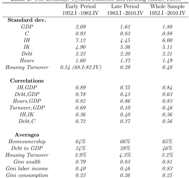
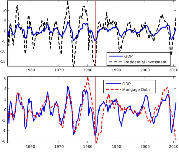
role could be relevant given two observations on the post-1980s period (see Figure 1 and Table 1). 46
First, the volatility of housing investment has fallen more than proportionally relative to GDP; 47
second, the correlations between mortgage debt and GDP and mortgage debt and aggregate 48
consumption have roughly halved, from0:78 to0:43and from 0:72 to0:37respectively.2 In line 49
with the data, we …nd that lower downpayments and larger idiosyncratic risk reduce the volatility 50
of housing investment, and reduce the correlation between mortgage debt and economic activity. 51
Lower downpayments provide a cushion to smooth housing demand; increase homeownership 52
rates, raising the number of people who do not change their housing consumption over the cycle 53
(relative to an economy with a large number of renters who can become …rst-time buyers); lead 54
to higher debt, creating a mechanism that weakens the correlation between output and hours. 55
Higher idiosyncratic risk makes wealth-poor individuals more cautious: these individuals adjust 56
consumption, hours, and housing by smaller amounts in response to aggregate shocks. This 57
mechanism is pronounced for housing purchases, since a house is a large item that is costly 58
to purchase and sell; and is reinforced by low downpayments, since low downpayments allow 59
people to borrow more, increasing the utility cost of buying and selling when net worth is lower. 60
Together, lower downpayments and higher risk can explain about15 percent of the reduction in 61
the variance of GDP,60 percent of the reduction in the variance of housing investment, and the 62
decline in the correlation between debt and GDP. 63
Debt and Housing in the Great Recession. During the 2007–2009 period, changes in …-64
nancial conditions are likely to have made the recession worse. In particular, the housing market 65
appears to have been held back – more than other sectors – by tighter credit conditions and 66
higher borrowing costs. In hindsight, it looks like housing did not stabilize the economy during 67
the recession. We use the model to determine the extent to which housing can smooth regular 68
business cycle shocks but amplify extremely negative ones, by de…ning “Normal Recessions” as 69
periods of low aggregate productivity, and “Great Recessions”periods of low aggregate produc-70
2 If one excludes the 2008-2010 period from the time-series, the decline in the volatility of housing investment and the decline in the correlation between debt and GDP are slightly larger.
tivity coupled with tight credit conditions. When we do so, we …nd an interesting nonlinearity: 71
higher risk and lower downpayments can make housing and debt more stable in response to 72
small positive and negative shocks (as in the Great Moderation), but can make it more fragile 73
in response to large negative shocks (as in the Great Recession). 74
Previous Literature. Two strands of literature study the role of housing in the macroecon-75
omy. On the one hand, business cycle models with housing –Greenwood and Hercowitz (1991), 76
Gomme, Kydland and Rupert (2001), Davis and Heathcote (2005), Fisher (2007) and Iacoviello 77
and Neri (2010) – match housing investment well, but abstract from a detailed modeling of 78
the microfoundations of housing demand; these models feature no wealth heterogeneity, no dis-79
tinction between owning and renting, and unrealistic transaction costs. On the other hand, 80
incomplete markets models with housing – Gervais (2002), Fernandez-Villaverde and Krueger 81
(2004), Chambers, Garriga and Schlagenhauf (2009), and Díaz and Luengo-Prado (2010) –have 82
a rich treatment of the microfoundations of housing demand, but ignore aggregate shocks: how-83
ever, because these papers model individual heterogeneity, they are better suited to study issues 84
such as debt, risk, and wealth distribution. 85
Our model combines both strands of literature. Others have also done so, albeit with a 86
di¤erent focus. Silos (2007) studies the link between aggregate shocks and housing choice, but 87
does not model the own/rent decision and assumes convex costs for housing adjustment.3 Fisher
88
and Gervais (2007) …nd that the decline in housing investment volatility is driven by a change 89
in the demographics of the population together with an increase in the cross-sectional variance 90
of earnings. Their approach sidesteps general equilibrium considerations. Kiyotaki, Michaelides 91
and Nikolov (2011) use a stylized life-cycle model of housing tenure to study the interaction 92
between borrowing constraints, housing prices, and economic activity. Favilukis, Ludvigson and 93
Van Nieuwerburgh (2009) use a two-sector RBC model with housing that also considers the 94
interaction between borrowing constraints and aggregate activity, but address a di¤erent set of 95
3 Under convex costs, housing adjustment takes the form of a series of small adjustments over a number of periods. Under our speci…cation, the homeowner’s housing stock follows an(S; s)rule, remaining unchanged over a long period and ultimately changing by a potentially large amount. See Carroll and Dunn (1997) for an early partial equilibrium model with(S; s)behavior for housing.
questions than we do. Finally, Campbell and Hercowitz (2005) study the impact of …nancial 96
innovation on macroeconomic volatility in a model with two household types. In their model, 97
looser collateral constraints weaken the connection between constrained households’ housing 98
investment, debt accumulation and labor supply through a mechanism that shares some features 99
with ours; however, their model does not study the interaction between life cycle, risk and housing 100
demand, which are important elements of our story. 101
2. The Model
102Our economy is a version of the stochastic growth model with overlapping generations of hetero-103
geneous households, extended to allow for housing investment, collateralized debt and a housing 104
rental market. Aggregate uncertainty is introduced in the form of a shock to total factor pro-105
ductivity. Individuals live at most T periods and work until age T < T:e Their labor endowment 106
depends on a deterministic age-speci…c productivity and a stochastic component. After retire-107
ment, people receive a pension. Each period, the probability of surviving from age a to a+ 1
108
is a+1. Each period a generation is born of the same measure of dead agents, so that the
to-109
tal population, which we normalize to 1; is constant. When an agent dies, he is replaced by a 110
descendant who inherits his assets. 111
At each point in time, agents di¤er by their age and productivity; moreover, we assume that 112
agents di¤er in their degree of impatience. We do so for two reasons: …rst, a large literature (see 113
Guvenen, 2011) suggests that preference heterogeneity may be an important source of wealth in-114
equality. For example, Venti and Wise (2001) study wealth inequality at the onset of retirement 115
among households with similar lifetime earnings and conclude that the dispersion must be at-116
tributed to di¤erences in the amount that households choose to save.4 Second, we want a model
117
that generates average debt and wealth dispersion as in the data, and a model with discount 118
factor heterogeneity works remarkably well in this regard (our robustness analysis discusses the 119
properties of the model with a single discount factor). 120
4 Krusell and Smith (1998) explore a heterogeneous-agents setting with discount rate heterogeneity which replicates key features of the data on the distribution of wealth.
Household Preferences and Endowments. Households receive utility from consumption 121
c, leisure l l (where l is the time endowment), and service ‡ows s from housing, which are 122
proportional to the housing stock owned or rented. The momentary utility function is: 123
u c; s; l l = logc+jlog ( s) + log l l . (1)
Above, = 1 if s = h > 0 (the individual owns), while < 1 if h = 0 (the individual rents). 124
The assumption for implies that a household experiences a utility gain when transitioning from 125
renting to owning, as in Rosen (1985) and Poterba (1992). We also assume that homeowners 126
need to hold a minimum size house h, and that rental units may come in smaller sizes than 127
houses, allowing renters to consume a smaller amount of housing services, as in Gervais (2002). 128
The log speci…cation over consumption and housing services follows Davis and Ortalo-Magné 129
(2011) who …nd that, over time and across cities, the expenditure share on housing is constant. 130
Time supplied in the labor market is paid at the wagewt. The productivity endowment of an
131
agent at ageais given by az;where ais a deterministic age-speci…c component andz is a shock 132
to the e¢ ciency units of labor, z 2 Ze fz1; :::; zn
g. The shock follows a Markov process with 133
transition matrix z;z0 = Pr (zt+1 =z0jzt =z) and stationary distribution (z) = Pr (zt=z) .
134
The total amount of labor e¢ ciency units Pni=1zi (zi) and of age-speci…c productivity values 135
PTe
a=1 a a are constant and normalized to one. From Te+ 1 onwards labor e¢ ciency is zero
136
(z = 0) and agents live o¤ their pension P and their accumulated wealth. Pensions are fully 137
…nanced through the government’s revenues from a lump-sum tax paid by workers.5 Total net
138
income at age a in period t is denoted by yat. Then:
139
yat =wt aztlt if a Te; yat =P if a >Te. (2)
Households start their life with endowmentsb0 and h0;the accidental bequests left by a dead
140
agent. They can trade a one–period bond b which pays a gross interest rate of Rt. Positive
141
amounts of this bond denote a debt position.6 Households cannot borrow more than a fraction
142
5 We crudely assume that the pension is the same for everyone. Allowing pensions to mimic something that looks like the actual Social Security system in the U.S. would make our model computationally intractable, since it would enlarge the state variables in the household problem to encompass their entire income history.
6 We refer to b as …nancial liabilities, and to b as …nancial assets. Because bonds are claims on aggregate capital, their return varies with the aggregate state.
mH <1 of their housing stock and a fractionmY of their expected earnings: 143 bt minfmHht; mY<t(yat;Rt; wt)g. (3) Above, <t(yat;Rt; wt) = yat + PT s=a+1 Et(ysjyat;wt)
(Rt)s a approximates the present discounted value of
144
lifetime labor earnings and pension.7 The motivation for this borrowing constraint is realism:
145
we want to study mortgage debt and we want to have a constraint which prevents the elderly 146
from borrowing too much late in life (when the present discounted value of earnings is low), 147
as in the data. The constraint is also consistent with typical lending criteria in the mortgage 148
market that take into account minimum downpayments, ratios of debt payments to income, 149
current and expected future employment conditions.8 Finally, we assume that an owner incurs a
150
transaction cost whenever he adjusts the housing stock: (ht; ht 1) = ht 1 if jht ht 1j > 0.
151
This assumption captures common practices in the housing market that require, for instance, 152
fees paid to realtors to be equal to a fraction of the value of the house being sold. Summing up, 153
households maximize expected lifetime utility: 154 E1 PT a=1 a 1 i a( Qa 1 =1 +1)u ca; sa; l la ; (4)
whereE1 denotes expectations at age a= 1, a is a deterministic preference shifter that mimics
155
changes in household size, and i is a household-speci…c discount factor. In the calibration, we
156
assume that households are born either impatient (low ) or patient (high ). 157
Financial Sector and Housing Rental Market. A competitive …nancial sector collects 158
deposits from households who save, lends to …rms and households who borrow, and buys capital 159
to be rented in the same period to tenants. The …nancial sector can convert the …nal good into 160
housing and capital at no cost. This assumption ensures that the consumption prices of housing 161
and capital are constant. Let pt be the price of one unit of rental services. Then a no-arbitrage
162
condition holds such that the net revenue from lending one unit of …nancial capital must equal 163
7 To compute<
t, we …x interest and wages at current values. To computeyat;we assumelt=l fort Te.
8 In the United States, lending institutions typically send a “Veri…cation of Employment” (VOE) form to the borrower’s employer to determine start date of employment, current and previous salary, and the probability of continued employment among other things.
the net revenue from renting one unit of housing capital, 164
pt = 1 Et((1 H)=Rt+1) (5)
at anyt; where H is the depreciation rate of the housing stock.9
165
Production. The goods market is competitive and characterized by constant returns to scale, 166
so that we consider a single representative …rm. Output is produced according to 167
Yt=AKt 1L 1
t ; (6)
whereKandLare total capital and labor input; is the capital share, andA2Ae fA1; ::; AnAg
168
is a shock to total factor productivity. This shock follows a Markov process with transition matrix 169
A;A0 = Pr (At+1 =A0jAt=A). The aggregate feasibility constraint requires that production of
170
the good Yt equals the sum of aggregate consumption Ct; investment in the stock of aggregate 171
capital Kt; investment in the stock of aggregate housing Ht = Hto+Htr; and total transaction
172
costs incurred by homeowners for changing housing stock, denoted by t:
173
Ct+Ht (1 H)Ht 1+ t+Kt (1 K)Kt 1 =Yt; (7)
with H and K denoting the depreciation rates of housing and capital, respectively.
174
The Household Problem and Equilibrium. Denote with t t(zt; bt 1; ht 1; ; a) the
175
distribution of households over earnings shocks, asset holdings, housing wealth, discount factors 176
and ages in period t: Without aggregate uncertainty, the economy would be in a stationary 177
equilibrium, with an invariant distribution and constant prices. Given aggregate volatility, this 178
distribution will change over time. When solving their dynamic optimization problem, agents 179
need to predict future wages and interest rates. Both variables depend on future productivity 180
and aggregate capital-labor ratio, which in turn are determined by the overall distribution of 181
9 One can interpret the marginal cost of one house to be 1 for the …nancial sector, since loanable funds can be converted into housing costlessly; and the marginal bene…t to be the sum of the current rental income, pt,
plus expected return next period,Et((1 H)=Rt+1), whereRtis the opportunity cost of funds for the …nancial
individual states. As a consequence, the distribution t –and its law of motion –is one of the
182
aggregate state variables that agents need to know in order to make their decisions (together 183
with total factor productivity). This distribution is an in…nite-dimensional object, and its law 184
of motion maps an in…nite-dimensional space onto itself, which imposes a crucial complication 185
for the solution of the model economy. To circumvent this problem, we adopt the strategy of 186
Krusell and Smith (1998) and let agents use one moment of the distribution –the aggregate 187
capital stock K – in order to forecast future prices. As documented in Appendix A, using one 188
moment only allows us to obtain a fairly precise forecast, as measured by theR2of the forecasting
189
equations, which are between 0:99 and 1.10
190
We write the household optimization problem recursively. The individual states are pro-191
ductivity zt; debt bt 1; and housing wealth ht 1. We assume that agents observe beginning of
192
period capital Kt 1 and approximate the evolution of aggregate capital and labor with linear
193
functions that depend on the aggregate shockAt:Denotext (zt; bt 1; ht 1; At; Kt 1)the vector
194
of individual and aggregate states. The dynamic problem of an age a household is: 195 Va(xt; i) = max Ih2f0;1gfI hVh a (xt; i) + 1 I h Vr a (xt; i)g; (8)
where Vah and Var are the value functions if the agent owns and rents, respectively, and Ih = 1
corresponds to the decision to own. The value of being a homeowner solves:
Vah(xt; i) = max ct;bt;ht;ltf au ct; ht; l lt + i a+1 P z0;A0 A;A0 z;z0Va+1(xt+1; i)g (9) s.t. ct+ht+ (ht; ht 1) =yat+bt Rtbt 1+ (1 H)ht 1; bt minfmHht; mY<tg; ct>0; lt2 0; l ; Kt=zK(Kt 1; At); Lt =zL(Kt 1; At). HerezK and
zLare linear functions inK
t 1;whose parameters depend on theAt. They denote
196
10 We have examined the robustness of our results by letting agents use both the aggregate capital stockK and the housing stockH in forecasting future prices, with nearly identical results, but at a higher computational cost. It is possible that higher moments of the wealth distribution could be both relevant in predicting future prices and yield di¤erent aggregate dynamics, so that our decision rules would describe a bounded rationality equilibrium, rather than a good approximation to the rational expectations equilibrium. Yet the evidence that adding H to the set of the state variables does not change aggregate dynamics leads us to be skeptical of this interpretation. See Young (2010) for an insightful discussion of these issues.
the law of motion of the aggregate state, which agents take as given. 197
The value of renting a house is determined by solving the problem:
Var(xt; i) = max ct;bt;st;ltf au ct; st; l lt + i a+1 P z0;A0 A;A0 z;z0Va+1(xt+1; i)g (10) s.t. ct+ptst+ (0; ht 1) = yat +bt Rtbt 1+ (1 H)ht 1; bt 0; ct >0; lt2 0; l ; ht= 0; Kt=zK(Kt 1; At); Lt =zL(Kt 1; At):
At the agent’s last age, VT+1(xT+1; ) = 0 for any (xT+1; ).
198
We are now ready to de…ne the equilibrium for this economy. 199
De…nition 2.1. A recursive competitive equilibrium consists of value functionsfVa(xt; )ga=1;::;T;t=1;::;1;
200
policy functions fIh
a(xt; ); ha(xt; ); sa(xt; ); ba(xt; ); ca(xt; ); la(xt; )g for each ; age
201
and period t, prices Rt, wt and pt; aggregate quantities Kt; Lt; Hto and Htr for each t; taxes
202
and pensions P;and laws of motionzK and
zL such that at anyt:
203
Agents optimize: Given Rt, wt; pt; and the laws of motion zK and zL, the value functions
204
solve the individual’s problem, with the corresponding policy functions.
205
Factor prices and rental prices satisfy:
Rt 1 + K = At(Kt 1=Lt) 1; (11) wt = (1 )At(Kt 1=Lt) ; (12) pt = 1 Et((1 H)=Rt+1). (13) Markets clear: Lt= R la(xt; ) aztd t (labor market), (14) Ct+Ht (1 H)Ht 1 + t+Kt (1 K)Kt 1 =Yt (goods market) (15)
where Ht and t are de…ned as: Ht =Hto+Htr= R Iah(xt; )ha(xt; )d t+ R (1 Iah(xt; ))sa(xt; )d t, (16) t = R (ha(xt; ); ht 1)d t: (17)
The government budget is balanced: 206 PTe a=1 a = PT a=Te+1 aP. (18)
The laws of motion for the aggregate capital and aggregate labor are given by
207
Kt=zK(Kt 1; At); Lt =zL(Kt 1; At). (19)
Appendix A provides the details on our computational strategy. 208
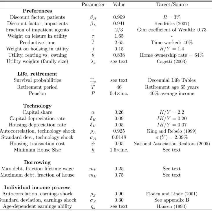
3. Calibration
209Our calibration is summarized in Table 2. One period is a year. Agents enter the model at 210
age21; retire at age 65; and die no later than age 90. The survival probabilities correspond to 211
the survival probabilities for men aged 21-90 from the U.S. Decennial Life Tables for 1989-1991. 212
Each period, the measure of those who are born is equal to the measure of those who die. The 213
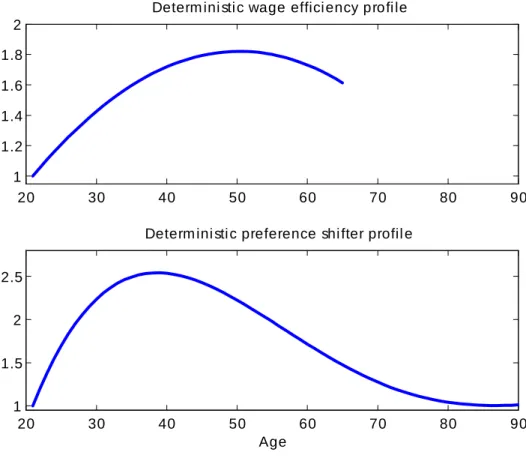
age polynomial a, which captures the e¤ect of demographic variables in the utility function,
214
is taken from Cagetti (2003) and approximated using a fourth-order polynomial (see Figure 2). 215
After normalizing the household size to 1 at age 21, the household size peaks at 2:5 at age 40, 216
and declines thereafter. 217
We take the deterministic pro…le of e¢ ciency units of labor for males aged21 65from Hansen 218
(1993) and approximate it using a quadratic polynomial (see Figure 2). Upon retirement, an 219
agent receives a pension equal to 40 percent of the average labor income.11 The idiosyncratic
220
shock to labor productivity is speci…ed as: 221
logzt= Zlogzt 1+ Z 1 2Z
1=2
"t; "t N ormal(0;1), (20)
which we approximate with a three-state Markov process following Tauchen (1986). There is 222
a vast literature on the nature and speci…cation of a parsimonious yet empirically plausible 223
income process: the bulk of the studies (see Guvenen, 2011) look at earnings (rather than wages) 224
11 Queisser and Whitehouse (2005) report that average pensions for males in the United States are 40 percent of the economy-wide average earnings.
and estimate persistence coe¢ cients ranging from0:7 to 0:95. Exception are Floden and Lindé 225
(2001), who use PSID data to estimate an AR(1) process for wages similar to ours and …nd 226
an autocorrelation coe¢ cient of 0:91; and Card (1991), who …nds an AR(1) coe¢ cient of 0:89. 227
Based on this evidence, we set Z = 0:9; and conduct robustness analysis in Section 8, based 228
on evidence from other studies that we review in Appendix B. The standard deviation of the 229
labor productivity process is set at Z = 0:30(see Appendix B). Later, we increase Z to 0:45
230
to capture the increased earnings volatility of the 1990s, and to study the consequences for 231
macroeconomic aggregates of increased risk at the household level, as emphasized by Mo¢ tt and 232
Gottschalk (2008) and Dynan, Elmendorf and Sichel (2007). 233
We assume that there are two classes of households, a “patient”group with a discount factor 234
of 0:999 (one third of the population) and an “impatient” group with a discount factor of0:941
235
(two thirds of the population). The high discount factor pins the average real interest rate down 236
to 3 percent. The low discount factor is in the range of estimates in the literature (see, for 237
instance, Hendricks, 2007). The gap between discount rates and the relative population shares 238
deliver a Gini coe¢ cient for wealth around 0:75, close to the data. In Section 8 we discuss the 239
properties of the model when we assume that all people have identical discount rates. We set 240
= 1:65and the endowment of time l = 2:65; these parameters imply that time spent working 241
is40 percent of the agents’time. 242
We set the weight on housing in utility at j = 0:15; and the depreciation rate for housing 243
H = 0:05. These parameters yield average housing investment to private output ratios around
244
7 percent, and a ratio of the housing stock to output 1:4. These values are in accordance with 245
the National Income and Product Accounts and the Fixed Assets Tables.12 Finally, the housing 246
transaction cost is set at = 5% based on estimates from the National Association of Realtors 247
12 The NIPA Fixed Asset Tables indicate depreciation rates for housing ranging from 1.2 to 4.5 percent, depending on the type of structure and its use (see Fraumeni, 1997). We choose a slightly higher value because we want to account for unmeasured labor time that is used to repair, renovate, or maintain or improve the quality of housing at a given location (Peek and Wilcox, 1991); because higher values are typically considered in the existing literature, especially when housing is broadly interpreted to include consumer durables (Chambers, Garriga and Schlagenhauf, 2009, Gervais 2002, and Díaz and José Luengo-Prado, 2010); and because a higher depreciation rate (5 percent instead of 2 percent, say) reduces the extent to which aggregate housing tends to decrease on impact following a positive aggregate technology shock in a model with two capital goods.
(2005).13 Section 8 conducts robustness analysis for alternative values of and
H.
248
We set = 0:26 and K = 0:09: These values yield an average capital to output ratios
249
around2:2 and average business investment to output ratios around20 percent. The aggregate 250
shock is calibrated to match the standard deviation of output in the data for the period 1952-251
1982. We use a Markov-chain speci…cation with seven states to match the following …rst-order 252
autoregression for the log of total factor productivity: 253
logAt= AlogAt 1+ A 1 2A
1=2
"t; "t N ormal(0;1). (21)
We set A = 0:925 and A = 0:0148. After rounding, the …rst number mimics a quarterly
254
autocorrelation rate of productivity of0:979;as in King and Rebelo (1999). The second number 255
is chosen to match the standard deviation of model output to its data counterpart. 256
Our baseline calibration sets the maximum loan-to-value ratio mH at 0:75. We increase mH
257
to 0:85 in the calibration for the late period. The value of mY is set at 0:25 in the baseline
258
and raised to 0:5 in the late period: with these numbers, the income constraint only binds 259
late in life, preventing old homeowners from borrowing. Aside from this, our choice for mY is of
260
small importance for the model dynamics. Lastly, the minimum-size house available for purchase 261
(h) costs1:5times the average annual pre-tax household income.14 Together with the minimum
262
house size, the parameter that has a large impact on homeownership is the utility penalty for 263
renting ( ). We set = 0:838 to obtain a homeownership rate of 64percent, as in the data for 264
the period 1952-1982. 265
4. Steady-State Results
266Household Behavior. At each stage in the life, the household chooses consumption, saving, 267
hours, and housing investment by taking into account current and expected income, and liquid 268
13 The National Association of Realtors estimates that average commission rates (excluding houses sold without brokers, which account for about 10 to 25 percent of existing home sales, according to media reports, reports of the National Association of Realtors, and academic studies) range from4:3 to 5:4 percent, based on 2004 data documenting a $65 billion brokerage industry and an existing home sales volume of $1.35 trillion.
14 According to the 2009 American Housing Survey, only 20 percent of total owner-occupied units have a ratio to current income less than 1.5.
assets and housing position at the beginning of the period. Here, we mostly focus on housing 269
decisions, since other features of the model are in line with existing models of life-cycle consump-270
tion and saving behavior. We defer illustrating labor supply behavior to the next section, when 271
we discuss the model dynamics in response to aggregate shocks. 272
It is simple to characterize the behavior of agents depending on whether they start the period 273
as renters or homeowners. For renters, the housing choice is as follows: given the initial state, 274
there is a threshold amount of liquid assets ( b in our notation) such that, if assets exceed the 275
threshold, renters become homeowners. Also, the larger initial liquid assets are, the less likely a 276
household is to borrow to …nance its housing purchase. 277
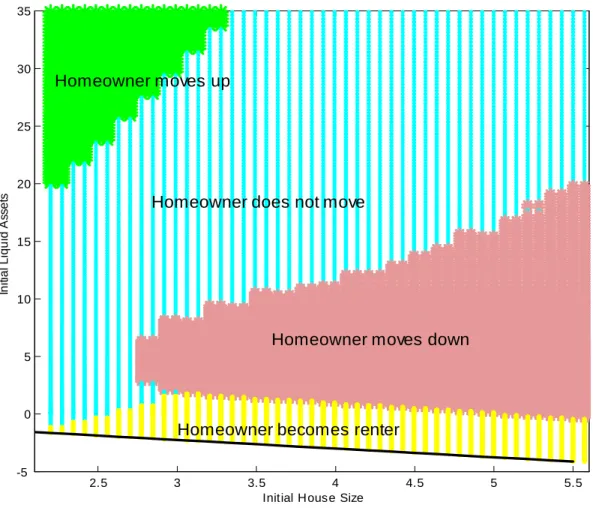
Homeowners can stay put, increase house size, downsize or switch to renting. Figure 3 plots 278
optimal housing choice as a function of initial house size and liquid wealth.15 The downward
279
sloping line plots the borrowing constraint that restricts debt from exceeding a fraction mH
280
of its housing stock. As the …gure illustrates, larger liquid assets trigger larger housing. In 281
addition, buying and selling costs create a region of inaction where the household keeps its 282
housing constant. If liquid wealth falls, the household either downsizes or switches to renting. 283
One feature of the model is that, for a household with very small liquid assets, the housing 284
tenure decision is non-monotonic in the initial level of housing wealth. Consider, for instance, a 285
homeowner with liquid assets equal to about one. If the initial house size is small, the homeowner 286
does not change house size, since, given the small amount of assets, the house size is closer to 287
its optimal choice. If the initial house is medium-sized, the homeowner pays the adjustment cost 288
and, because of his low liquid assets, switches to renting. If the initial house size is large, it is 289
optimal to downsize, and to buy a smaller house. 290
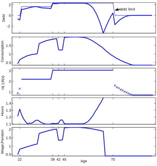
Life-Cycle Pro…les. Figure 4 plots a typical individual life-cycle pro…le in our model. We 291
choose an agent with a low discount factor since the behavior of an agent with low assets and 292
often close to the borrowing constraint best illustrates the main workings of the model. The 293
agent starts life as a renter, with little assets and low income. At the age of 22; he is hit by a 294
15The …gure is plotted for a patient agent who is entering retirement (65 years old), when aggregate productivity and the capital-labor ratio are equal to their average value.
positive income shock, saves in order to a¤ord the downpayment and buys a house a year after. 295
Prior to buying a house, the individual works more: the positive income shock raises the incentive 296
to work; and such incentive is reinforced by need to set resources aside for the downpayment. 297
Following a series of above average income shocks beginning at the age of 32; the agent buys a 298
larger house at the age of 39. This time, in order to a¤ord the larger house, the individual is 299
much closer to his borrowing limit. In particular, while he owns and is close to the borrowing 300
limit, hours move in the opposite direction to wage shocks, rising in bad times (age42), falling 301
in good times (age45): such mechanism is explained in detail in the next Section. As retirement 302
approaches, the agent pays back part of the mortgage, and works more. After retirement, at the 303
age of 70;he switches to a small rental unit, before dying at the age of 90. 304
One dimension where it is illustrative to compare the model with the data is the frequency 305
of housing adjustment for homeowners.16 Using the 1993 Survey of Income and Program Partic-306
ipation, Hansen (1998) reports that the median homeowner stays in the same house for about 8 307
years. Anily, Hornik, and Israeli (1999) estimate that the average homeowner lives in the same 308
residence for 13 years. The corresponding number for our model is 15 years.17 309
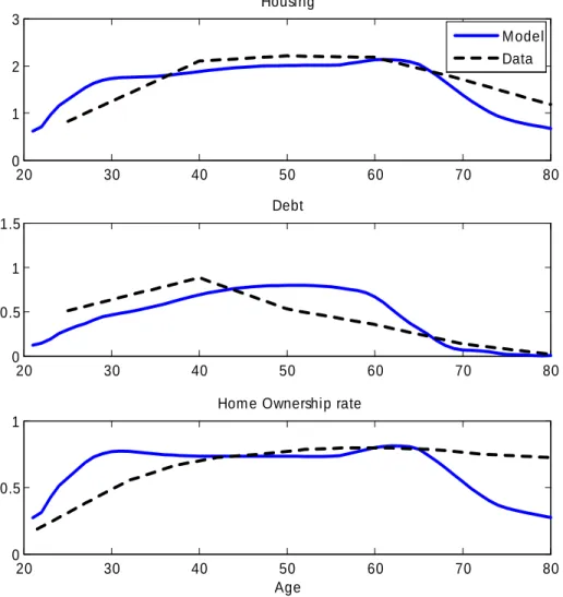
Figure5 compares the age pro…les of housing, debt and homeownership with their empirical 310
counterparts. Like the data, the model is able to capture the hump-shaped pro…les of these 311
variables. There are two discrepancies: as for mortgage debt, the model slightly underpredicts 312
debt early in life, and overpredicts debt later in life. The model also underpredicts homeownership 313
later in life: we believe that, late in life, the absence of any bequest motive and the need to 314
…nance consumption expenditure by selling the house more than o¤set the adjustment costs, 315
thus generating a sharp decline in homeownership. 316
The Wealth Distribution. Our model reproduces the U.S. wealth distribution quite well. 317
The Lorenz curves for the U.S. economy and for our model economy are reported in …gure 6. 318
16 In the model, renters change their housing position every period, since they face no cost in doing so. This assumption is in line with the data, that show that on average renters move about every two years.
17 We are aware, of course, of the di¢ culty in comparing the model with the data along this dimension: in the data, 15 percent of the moves are associated with a move to a di¤erent state, and 35 percent of the moves are associated with a move to a di¤erent county. Most of these moves are probably “moving shocks” rather than movements along the housing ladder.
The Gini coe¢ cient for wealth in the model is 0:73, and is about the same as in the data (equal 319
to 0:79). Our model still underpredicts wealth inequality at the very top of the distribution, 320
both for housing and for total wealth. However, the model does well at matching the fraction 321
of wealth (both housing wealth and overall wealth) held by the poorest 40 percent of the U.S. 322
population, which has essentially no assets and no debt. Instead, a model without preference 323
heterogeneity would do much worse: in Section 8we show that the Gini coe¢ cient for wealth in 324
the model with a single discount factor is0:53, much lower than in the data. 325
In the same vein, the model predicts a mortgage debt to GDP ratio that is roughly in line 326
with the data (0:31vs. 0:34) and a fraction of liquidity constrained agents that is consistent with 327
the available empirical estimates. Following Hall (2011), we take a model agent to be liquidity-328
constrained if the holdings of net liquid assets are less than two months (16.67% on an annual 329
basis) of income.18 Using this de…nition, 45% of households are liquidity constrained.19 Jappelli 330
(1990) estimates the share of liquidity constrained individuals to be 20%. Studies that have 331
combined self–reported measures of credit constraints from the Survey of Consumer Finances 332
with indirect inference from other datasets (such as the PSID), have typically found that 20
333
percent is more likely to be a lower bound. For instance, using evidence on the response of 334
spending to changes in credit card limits, Gross and Souleles (2002) argue that the overall 335
fraction of potentially constrained households is over two thirds. 336
5. Business Cycle Results
337We now illustrate the propagation mechanism of aggregate shocks. There are two aspects of 338
heterogeneity that matter for aggregate dynamics: one is exogenous, and re‡ects the assump-339
tion that individuals have di¤erent abilities, planning horizons, and utility weights. Because 340
other papers have studied these features in life-cycle models with aggregate shocks, we do not 341
18 Liquid assets are de…ned aslqas m
Hh0 b0:According to this de…nition, an owner(h0 >0)is not liquidity
constrained so long as it saves su¢ ciently more (borrows less) than the minimum downpayment in the house (lqas >0:1667y); a renter (h0 = 0) is not constrained if …nancial assets are su¢ ciently large (b0< 0:1667y).
19The baseline model predicts that70percent of renters and31percent of homeowners are liquidity constrained; and that67percent of impatient agents and2 percent of patient agents are liquidity constrained.
explore them in detail here.20 Instead, we focus on the endogenous component of heterogeneity,
342
which re‡ects the fact that individuals with di¤erent ages and income histories accumulate dif-343
ferent amounts of wealth over time; in turn, heterogeneity in wealth implies di¤erent individual 344
responses to the same shock. 345
Workings of the Model. We focus on the response of aggregate hours to a technology shock, 346
since movements in hours are the key element of the propagation mechanism in models that 347
rely on technology shocks as sources of aggregate ‡uctuations. In particular, we study how 348
the wealth distribution and its composition shape agents’ responses to shocks. To …x ideas, 349
consider a stripped-down version of the budget constraint of a working individual that keeps 350
wealth constant between two periods: bt = bt 1 and ht = ht 1.21 Abstracting from taxes and
351
pensions, this implies the following budget constraint: 352
ct=wt aztlt+ t; (22)
where t = (Rt 1)bt 1 Hht 1 measures the resources besides wages that can be used to
353
…nance consumption:22 the term(1 R)bis net interest income; the term Hhis the maintenance
354
cost required to keep housing unchanged. Di¤erent values of map into di¤erent positions of the 355
agents along the wealth distribution. For a wealthy homeowner (negative b), is positive and 356
large, and wage income is a small fraction of consumption c. For a renter, h = 0; in addition, 357
assuming that the renter is not saving, b = 0, so that = 0 too. For a homeowner with a 358
mortgage (positive b), is negative. Normalize a = 1 and set aside idiosyncratic shocks, so
359
that zt = 1 at all times. Assuming that stays constant, the log-linearized budget constraint
360
becomes, denoting with bx xt x
x ; where x is the steady-state value of a variable:
361
b
c= wl
c wb+bl . (23)
20 See for instance the work of Ríos-Rull (1996) and Gomme et al. (2004).
21 Obviously, the optimal decisions involve the joint choice of (1)consumption, (2) housing,(3) debt and(4) hours worked. By assuming that housing and debt remain constant across two subperiods, we can study the joint determination of consumption and hours by focusing on the budget constraint and the Euler equation for labor supply only. This is a reasonable assumption for small shocks (such as aggregate shocks).
22 Renters have constant shares of housing and nonhousing consumption, so thatc
t= (wt aztlt+ t)=(1 +j);
wherejis the ratio of housing expenditure to nondurable consumption. With minor modi…cations, the arguments in the text carry over to this case, since cannot be negative for renters:
This constraint can be interpreted as an equation dictating how much the household needs to 362
work to …nance a given consumption stream, given the wage. The larger the desired consumption 363
b
c; the larger the required hoursbl needed to …nance the consumption stream, with an elasticity 364
of hours to consumption given by consumption–wage income ratio (c=wl) . For a wealthy 365
individual, is high and larger than one, since labor income is a small share of total earnings; 366
for a renter without assets, = 1; for an indebted homeowner, <1, re‡ecting the need to use 367
part of the earnings to …nance maintenance costs and to service the mortgage. In other words, 368
a wealthy person needs to increase hours by more than 1 percent to …nance a 1 percent rise 369
in consumption, since labor income is less than consumption; an indebted homeowner needs to 370
increase hours by less than1 percent to …nance a 1 percent rise in consumption, because of the 371
leverage e¤ect; a renter without assets needs to increase hours1 for 1with consumption. 372
The other key equation determining hours is the standard labor supply schedule. Letting 373
denote the steady-state Frisch labor supply elasticity, this curve reads as 374
b
l = (wb bc). (24)
Combining equations 23 and 24 yields: 375
b
l = 1
+ wb. (25)
Take the wage as the exogenous driving force of the model, since an exogenous rise in productivity 376
exerts a direct e¤ect on the wage. Whether the rise in the wage leads to an increase in hours 377
depends on whether the consumption–wage income ratio, ; is smaller or larger than one. In 378
other words, all else equal, borrowers ( <1) are more likely to reduce hours following a positive 379
wage shock, whereas savers ( >1) are more likely to increase them. 380
For the economy as a whole, the response of total hours to a wage change will be an average 381
of the labor supply responses of all households. If individual labor schedules were linear in 382
net wealth, the aggregate labor supply response would be linear in average wealth, and wealth 383
distribution would not a¤ect labor supply. There are, however, two main forces that undo the 384
linearity. First, retirees do not work, so any transfer of wealth to and from them could a¤ect how 385
the workers respond to wage shocks. Second, the interaction between borrowing constraints and 386
housing purchases creates an interesting nonlinearity. Above, we have assumed that households 387
do not change wealth in response to a shock in the wage. However, if households switch from 388
renting to owning (or if they increase their house size) in good times, they typically need to 389
save for the downpayment. This increases the incentive to work: intuitively, if the individual 390
wants to keep consumption constant when he buys the house, he needs to work more hours. This 391
e¤ect creates comovement between hours and housing purchases.23 In particular, it reinforces the
392
correlation between hours and housing demand in periods when a large fraction of the population 393
has, all else equal, low net worth. 394
Business Cycle Statistics. In HP-…ltered U.S. data, the variability of housing investment is 395
large, with a standard deviation that is between three and four times that of GDP (in the period 396
1952-1982). Also, housing investment is procyclical, with a correlation with GDP around 0:9. 397
Together, these two facts imply that the growth contribution of housing investment to the busi-398
ness cycle is larger than its share of GDP. Household mortgage debt is strongly procyclical from 399
1952to1982, but it becomes less procyclical after, with a correlation with GDP that drops from 400
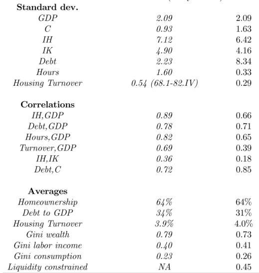
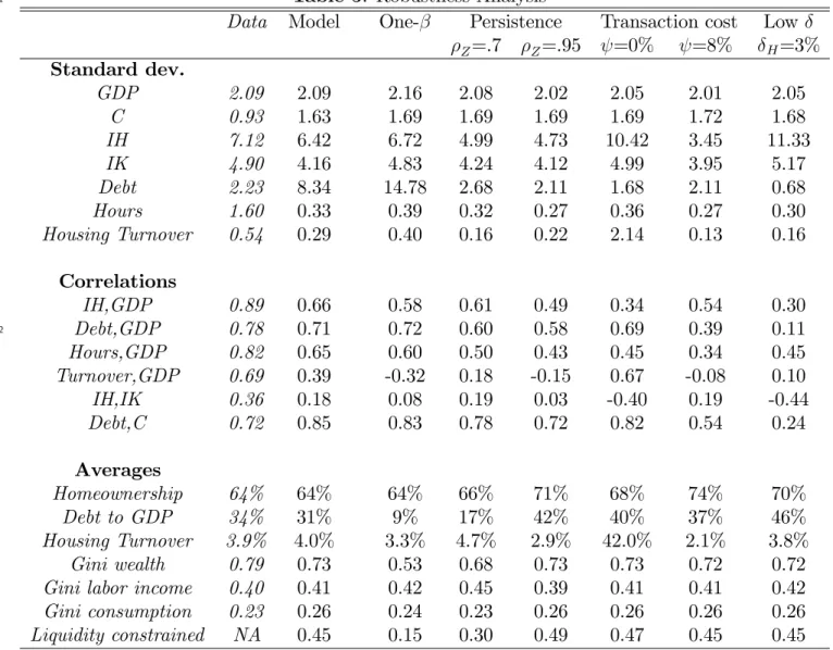
0:78to0:43. Table 3compares the benchmark model with the data. Overall, our baseline model 401
does a good job in reproducing the relative volatility of each component of aggregate demand. 402
In particular, it can account for about three quarters of the variance of housing investment. On 403
the contrary, the model overpredicts the volatility of aggregate consumption. The volatility of 404
business investment is only slightly lower than in the data. As in many RBC models without an 405
extensive margin of work and without direct shocks to the labor supply, our model underpredicts 406
the volatility of hours (0:33percent in the model, 1:6percent in the data). 407
Turning to debt, the model does well in reproducing its cyclical behavior.24 The key to this
408
result is that the bulk of the debt holders (mostly impatients) upgrades housing in good times 409
23 The limiting case of zero forced savings would be the case in which no downpayment is needed to buy a house. In that case the individual can keep consumption constant at the time of the purchase without increasing hours worked if transaction costs are zero. If the individual has to pay the transaction cost, this provides an incentive to work more at the time of the purchase. Campbell and Hercowitz (2005) propose a similar argument to discuss the relationship between hours and durable purchases.
24 We de…ne household debt asD
t=
R
by taking out a (larger) mortgage. At the same time, the model overpredicts the volatility of 410
debt itself: the standard deviation of the model variable is about four times larger than in the 411
data. We suspect that the reason for the higher volatility of debt in the model has to do with 412
the simplifying assumption that only one …nancial asset is available, whereas in the data some 413
households (especially the wealthy) own simultaneously a mortgage and other …nancial assets. If 414
debt of low-wealth households is more volatile than debt of high-wealth households, our model 415
variable can exhibit more volatility than its data counterpart. 416
One dimension where it is useful to compare the model with the data pertains to home sales. 417
In our model, we count a sale as every instance in which a household pays the transaction cost to 418
change its housing: this involves own-to-own, rent-to-own and own-to-rent transitions. By this 419
metric, the average turnover rate in the model (the ratio of sales to total houses) is 4 percent, 420
a number that matches the3:9 percent in the data.25 Moreover, the model correlation between 421
turnover rate and GDP is0:39, and the standard deviation is 0:29. The corresponding numbers 422
from the data are 0:69 and 0:54. The positive correlation between sales and economic activity 423
that the model captures re‡ects the presence of liquidity constraints: when the economy is in 424
recession and household balance sheets have deteriorated, the potential movers in the model …nd 425
their liquidity so impaired, whether they are owners or renters, that they are better o¤ staying 426
in their old house rather than attempting to move and paying the transaction cost. 427
6. E¤ects of Lower Downpayments and Higher Risk
428Having shown above that the model roughly captures postwar U.S. business cycles, we now 429
consider the implications of two experiments. In the …rst, we lower the downpayment from25to 430
15 percent. In the second, we increase the idiosyncratic risk faced by households, changing the 431
unconditional standard deviation of income Z from 0:30 to 0:45. Our experiment is intended
432
to mirror two of the main changes that have occurred in the U.S. economy since the mid 1980s. 433
25 The turnover rate in the data is constructed as the sum of sales of existing single-family homes (source: National Association of Realtors) plus new single-family homes sold (from Census Bureau), divided by the total housing stock (from Census Bureau). The series starts in 1968.
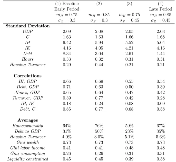
The model results are in Table 4. 434
A Decline in Downpayments. Lower downpayments (column 2 in Table 4) lead to an in-435
crease in the homeownership rate (from64to 76percent) and to a higher level of debt (from 31
436
to50percent of GDP). Smaller downpayments allow more housing ownership among the portion 437
of the population with very little net worth. While debt is higher, the increase in homeowner-438
ship works to keep total wealth inequality unchanged: …nancial wealth inequality is higher, but 439
housing wealth inequality is lower. Turning to business cycles, the rise inmH tends to reduce the
440
volatility of housing investment, from6:42to 5:94percent, for two reasons. The …rst reason has 441
to do with adjustment costs: on average, because of adjustment costs, homeowners modify their 442
housing little over time relative to renters. The second motive operates through the interaction 443
of labor supply and housing purchases. As we explained above, indebted homeowners are more 444
likely, compared to renters, to reduce hours in response to positive technology shocks, so their 445
presence dampens aggregate shocks. Therefore, the higher homeownership rate induced by looser 446
borrowing constraints reduces aggregate volatility.26
447
An Increase in Individual Earnings Volatility. Column 3 in Table 4 shows that, following 448
a rise in Z, the homeownership rate falls from 64 to 59percent: higher risk makes individuals
449
more reluctant to buy an asset that is costly to change. All else equal, the lower homeownership 450
rate would tend to increase the volatility of housing investment, since renters change housing 451
consumption more often. However, this e¤ect is more than o¤set by the behavior of those who 452
remain homeowners: these people are now more reluctant to change their housing consumption 453
(relative to a world with less individual risk). This occurs because modifying housing, in the 454
26 A similar intuition has been proposed in Campbell and Hercowitz (2005), who show that …nancial innovation alone can explain more than half of the reduction in aggregate volatility in a model with borrowers and lenders and downpayment constraints. Aside from modeling di¤erences (our model considers the owning/renting margin and addresses issues related to life cycle, lumpiness and risk that are absent in their setup), the intuition they o¤er for their result carries over to our model, but we …nd that the e¤ect of lower downpayment requirements is quantitatively smaller. We conjecture that the di¤erences depend on one modeling assumption: in our setup, indebted homeowners mitigate aggregate volatility, but this e¤ect is partly o¤set by the wealthier homeowners (the creditors) who tend to increase aggregate volatility by working relatively more in response to positive aggregate shocks; instead, Campbell and Hercowitz assume that labor supply of wealthy homeowners is constant, thus killing this o¤setting mechanism.
presence of transaction costs, depletes holdings of liquid assets and increases the utility cost of 455
a negative idiosyncratic shock, thus increasing the option value of not adjusting the stock for 456
given changes in net worth. Quantitatively, the higher earnings volatility reduces the standard 457
deviation of housing investment from 6:42 to 5:52 percent. Moreover, higher income volatility 458
also reduces the sensitivity of debt to aggregate shocks, since debt is used to …nance housing 459
purchases, and housing purchases respond less to shocks. 460
Combining Lower Downpayments and Higher Volatility. The last column of Table 4
461
shows the e¤ects of combining lower downpayments and higher volatility. The two forces together 462
predict an increase in homeownership rates from 64 to 67 percent. The data counterpart is a 463
two percentage points rise, from64 to66 percent. Moreover, the joint e¤ect of these two forces 464
makes debt less procyclical, as in the data. The correlation between debt and output falls from 465
0:71 to 0:39; a change that is remarkably similar to the data (from 0:78 to 0:43, see Table 1).27 466
Together, lower downpayments and high idiosyncratic volatility reduce the standard deviation 467
of GDP from2:09 to2:03 percent, and the standard deviation of housing investment from 6:42
468
to5:04. percent. When these numbers are compared to the data, the two changes combined can 469
account for 13 percent of the variance reduction in GDP and about 60 percent of the variance 470
reduction in housing investment. 471
Our interpretation of these results is as follows: in response to lower downpayments and higher 472
income volatility, leveraged households become more cautious in response to aggregate shocks, 473
thus changing less borrowing and housing demand when aggregate productivity changes.28 This
474
is especially true for housing, relative to other categories of expenditure, since housing is a highly 475
durable good and is subject to adjustment costs. Because individuals are reluctant to adjust their 476
housing consumption during uncertain times, the sensitivity of hours to aggregate shocks falls 477
27 Likewise, the correlation between debt and consumption falls in the model from0:85to0:58;a decline similar to the data (from0:72to 0:37).
28 Higher uncertainty in itself reduces the willingness to borrow, whereas lower downpayments lead to an increase in debt. In our baseline calibration, the second e¤ect dominates –as shown in table 4, the ratio of debt to GDP rises from0:31to 0:35when both changes are present. As a consequence, in the late period individuals are more cautious, even if they hold more debt. For this reason, the fraction of liquidity constrained households in the model falls from45to38percent.
too. As a consequence, even if the volatilities of consumption and business investment are not 478
changing, total output is less volatile. 479
In Figure 7, each panel shows average debt, hours and housing positions by age in the lowest 480
and the highest aggregate state. The top panel plots the calibration with high downpayments 481
and low idiosyncratic risk (the period 1952-1982): changes in the aggregate state generate large 482
di¤erences in debt, housing and hours. The bottom panel plots the case with low downpayments 483
and high idiosyncratic risk (the period 1983-2010): changes in the aggregate state generate 484
smaller di¤erences in debt, housing, and hours, thus illustrating how these variables become less 485
volatile and less procyclical. 486
Figure 8 plots the model dynamics when technology switches from its average value to a 487
higher value (about 1 percent rise) in period 1. The responses are larger in the earlier period. 488
On impact, housing falls before rising strongly in period 1. This result is well known in the 489
household production literature (see, for instance, Greenwood and Hercowitz 1991 and Fisher 490
2007). In models with housing and business capital, business capital is useful for producing more 491
types of goods than housing capital. Hence, after a positive productivity shock, the rise in the 492
marginal product of capital implies that there is a strong incentive to move resources out of the 493
housing to build up business capital, and only later is housing accumulated. The key aspect 494
to note here is that higher idiosyncratic risk and lower downpayment requirements dampen the 495
incentive to adjust housing capital, so that housing investment becomes less volatile. 496
Our result that higher individual uncertainty reduces the volatility of aggregate housing 497
investment echoes the results of papers that study how durable purchases respond to changes 498
in income uncertainty in (S; s) models resulting from transaction costs. Eberly (1994), using 499
data from the Survey of Consumer Finances, considers automobile purchases in presence of 500
transaction costs: she …nds that higher income variability broadens the range of inaction, and 501
that the e¤ect is larger for households that are liquidity constrained. Foote, Hurst and Leahy 502
(2000) …nd a similar result using data on car holdings from the Consumer Expenditure Survey, 503
and o¤er an explanation that involves the presence of liquidity constraints and precautionary 504
saving: adjusting the capital stock for people with low levels of net worth depletes holdings of 505
liquid assets and increases the utility cost of a negative idiosyncratic shock, thus increasing the 506
option value of not adjusting the stock for given changes in net worth. 507
7. Debt and Housing in a Great Recession Experiment
508The …nding that housing and debt are less sensitive to aggregate shocks when downpayments are 509
low and idiosyncratic risk is high can account for part of the Great Moderation, but is at odds 510
with the events of the 2007-2009 …nancial crisis, when both housing and debt fell substantially. 511
Explaining the crisis is beyond the scope of this paper, but in this section we show that our 512
model expanded to take into account the “credit crunch” can generate, at least qualitatively, 513
the observed response of housing and debt in the Great Recession. We extend the stochastic 514
structure of the model so that, when the worst technology shocks hit, credit standards get tighter 515
too, in the form of lower loan-to-value ratios and higher costs of …nancial intermediation (higher 516
borrowing interest rates). In other words, consistent with the post-2007 evidence,29 recessions are
517
now a combination of negative …nancial and negative technology shocks occurring simultaneously. 518
We implement this scenario by assuming that the maximum loan-to-value ratiomH changes over
519
time as a function of total factor productivity,At: formally, mH;t =mH(At):Moreover, we also
520
introduce an additional cost of …nancial intermediation in the form of an interest rate premium 521
rpt =rp(A
t)to be paid by debtors. The budget constraint for a home buyer become respectively:
522
ct+ht+ (ht; ht 1) =yat+bt (Rt+I(bt 1 >0)rpt)bt 1+ (1 H)ht 1 (26)
523
with bt min (mH;tht; mY<t); ct>0; lt2 0; l ; (27)
where I(bt 1 > 0) is the indicator function equal to 1 if the household is a net debtor, 0
oth-524
erwise. The state vector xt remains unchanged with respect to the benchmark model, and so
525
does the equilibrium de…nition. In the calibration, we let mH drop by 6 percentage points in
526
correspondence of the two lowest values of At, and leave it constant for all other values of At.30
527
29Jermann and Quadrini (forthcoming) document that credit shocks have played an important role in capturing U.S. output during the last decades.
30 Total factor productivity is discretized using a 7-state Markov chain (see Appendix). For the lowest two aggregate productivity levels: in the period 1952-1982,mH;t= 0:70, and in the period 1983-2010,mH;t= 0:80.
We set the values of the interest rate premium at0:75%for the two lowest aggregate productivity 528
realizations, in both periods (rp is equal to zero for all other values of A t).
529
We …nd that this simple modi…cation of the model can qualitatively account for the behavior 530
of housing and debt in the most recent events. Figure9 shows the impulse responses to positive 531
and negative productivity shocks, comparing the early period with the late period (de…ned as in 532
the baseline exercise). In the late period, debt, housing and GDP respond less to positive shocks, 533
so that one …nds evidence of the Great Moderation so long as the economy is lucky enough not 534
to be hit by (too negative) negative shocks. When the worst recessionary shocks hit, however, 535
the decline in debt and in housing purchases are considerably larger in the late period than in 536
the early period. In other words, when leverage is high, the housing sector can better absorb 537
“small”business-cycle shocks, but becomes more vulnerable to large negative shocks that result 538
in a credit crunch: these shocks cause highly-leveraged households to sharply reduce their debt 539
and housing purchases.31
540
8. Sensitivity Analysis
541We discuss in this section four alternative versions of the model where we modify the calibration 542
used in our benchmark. 543
Discount Factor. To analyze the model with homogeneous discounting, we modify the cali-544
bration for the discount factor ( = 0:978) and for the relative utility from renting ( = 0:922) 545
in order to achieve the same homeownership rate and interest rate as in our baseline. As shown 546
in Table5; the volatilities of housing investment and output are now slightly higher than in the 547
baseline calibration, but the correlations of housing investment and of hours with output fall: this 548
result occurs because fewer people are close to the borrowing limit (only 15 percent of households 549
are liquidity–constrained) and in need of increasing hours to …nance the downpayment in good 550
times. In addition, with a single discount factor, very few people hold debt in equilibrium, and 551
the distribution of wealth is more egalitarian than in the data: the Gini coe¢ cient for wealth is 552
0:53, lower than in the data and in the benchmark model. The model predicts, unlike the data, 553
a negative correlation between turnover and GDP: with a single discount rate, more housing 554
capital reallocation occurs in bad times. 555
Persistence of the Income Process. One key parameter is the persistence of income shocks. 556
Our benchmark sets Z = 0:9. The robustness analysis in Table 5 shows that, holding total
557
income risk constant, some of the model properties are a non–monotonic function of Z. When 558
the shocks are not very persistent ( Z = 0:7), the equilibrium level of debt is relatively low,
559
fewer people are at the liquidity constraint, and debt and housing investment are less volatile 560
and slightly less cyclical. Conversely, when income shocks are highly persistent ( Z = 0:95), 561
more people are liquidity constrained, but more people are lucky for a spell long enough to 562
a¤ord the downpayment for a house and to keep housing and debt relatively unchanged in 563
response to shocks.32 In other experiments not reported in the Table, we have found that only 564
for intermediate values of the persistence coe¢ cient (between 0:85 and 0:92), can the model 565
account for both the high volatility of housing investment and the high correlation of debt with 566
economic activity. Moreover, for values of Z above0:95;housing turnover is negatively correlated
567
with GDP, and housing is negatively correlated with business investment. 568
Housing Transaction Costs. We consider two polar cases, zero and high transaction costs. 569
With no transaction costs, the standard deviation of housing investment, which is6:42percent in 570
the baseline, rises to10:42percent (see Table 5).33 Because houses are less risky, homeownership 571
rises, from64 to 68 percent. Aggregate volatility falls: housing and nonhousing capital become 572
closer substitutes as means of saving, and the higher volatility of housing investment is o¤set 573
by the reduced covariance between housing and nonhousing investment. The correlation between 574
32 To keep our experiments simple and easier to interpret, we do not attempt here at recalibrating some of the other parameters in order to match the same targets as in the benchmark model.
33 Thomas (2002) argues that lumpiness of …xed investment at the level of a single production unit bears no implications for the behavior of aggregate quantities in an otherwise standard RBC model. Her argument rests on the representative household’s desire to smooth consumption over time, a desire that undoes any lumpiness at the level of the individual …rm. Our sensitivity analysis shows that there are di¤erences between the models with and without adjustment cost. Adjustment costs imply smaller housing adjustment at the aggregate level, but larger housing adjustments (when they occur) at the individual level.