Using Unsupervised Deep Learning Technique
for Monocular Visual Odometry
QIANG LIU , RUIHAO LI, HUOSHENG HU , (Senior Member, IEEE), AND DONGBING GU School of Computer Science and Electric Engineering, University of Essex, Colchester CO4 3SQ, U.K.
Corresponding author: Qiang Liu ([email protected])
ABSTRACT Deep learning technique-based visual odometry systems have recently shown promising results compared to feature matching-based methods. However, deep learning-based systems still require the ground truth poses for training and the additional knowledge to obtain absolute scale from monocular images for reconstruction. To address these issues, this paper presents a novel visual odometry system based on a recurrent convolutional neural network. The system employs an unsupervised end-to-end training approach. The depth information of scenes is used alongside monocular images to train the network in order to inject scale. Poses are inferred only from monocular images, thus making the proposed visual odometry system a monocular one. The experiments are conducted and the results show that the proposed method performs better than other monocular visual odometry systems. This paper has made two main contributions: 1) the creation of the unsupervised training framework in which the camera ground truth poses are only deployed for system performance evaluation rather than for training and 2) the absolute scale could be recovered without the post-processing of poses.
INDEX TERMS Monocular visual odometry, unsupervised deep learning, recurrent convolutional neural networks.
I. INTRODUCTION
Visual odometry (VO) has drawn enormous attentions from both robotics and computer vision communities during the last decades. It studies how a robot can estimate its move-ment relative to a rigid scene through a camera (monocular, stereo or omnidirectional) attached to it [1]. The traditional VO systems consist of image correction, feature extraction and representation, feature matching, transformation estima-tion and pose graph optimizaestima-tion. They have shown some outstanding performance through careful design and adjust-ment step by step, which are very costly [2]. The technique has been widely applied to augmented reality (AR), mobile robots, wearable devices, etc.
Deep learning based VO systems developed in recent years [3]–[6] have already shown promising performance in terms of both translation and rotation estimation accuracy. Ground truth poses of each input frame need be acquired beforehand and fed into these networks for training. However, ground truth poses are difficult and expensive to obtain. In some systems, ground truth poses are even inferred
The associate editor coordinating the review of this manuscript and approving it for publication was Yu-Huei Cheng.
and obtained by labeling collected images with traditional VO or SLAM algorithms, which is an ill-posed problem.
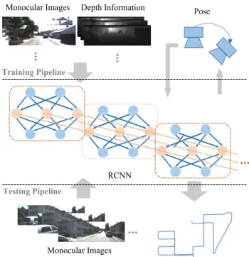
This paper proposes an unsupervised training framework which does not require the ground truth poses of a camera in any form for training. Instead, the ground truth poses of the camera are only used for performance evaluation. Therefore, such unsupervised training eliminates the need of the labor-intensive image labeling process. In addition, the performance of our system can be easily improved by further training with larger unlabeled dataset. Fig.1gives an overview of our proposed VO system. The training dataset includes a pair of monocular and depth images. Transforma-tion matrices generated by the network are used to calculate losses. Parameters in the network are then optimized by min-imizing these losses. We use consecutive monocular images for testing. The network directly yields poses on an absolute scale.
Monocular VO is one of the most popular VO cate-gories depending on the camera setup. However, the absolute scale cannot be obtained based solely on monocular images. Either external information or prior knowledge (ground truth pose) is required at some stage during reconstruction or/and training. In robotics, one typical way of obtaining scale
18076
2169-35362019 IEEE. Translations and content mining are permitted for academic research only.
FIGURE 1. Overview of the proposed visual odometry system.
during reconstruction is by combining a monocular cam-era with other sensors such as Inertial Measurement Unit (IMU) and optical encoder. Another solution is by providing depth information of the scene in some way. This can be achieved via employing RGB-D sensors (Microsoft Kinect, Asus Xtion Pro, etc.) [7]–[9], stereo cameras [10], [11] or 3D LiDARs [12], [13]. This solution has been widely deployed in self-driving cars and smart phones. In this paper, we feed monocular images and depth information obtained from 3D LiDARs into the training pipeline to inject abso-lute scale and only use monocular images during testing. We focus on the problem of continuously localizing a monoc-ular camera on an absolute scale for the purpose of locating people or robots.
As the global pose graph is obtained from a sequence of images gradually rather than through a single calculation, the deep learning network should consider the previous com-putations before it outputs the pose of the current frame. Thus, this paper proposes the use of a Recurrent Convolutional Neural Network (RCNN) to meet such requirements, which is based on the methodologies presented by Wanget al.[4] and Liet al. [14]. More specifically, it is a combination of a Convolutional Neural Network (CNN) for differentiating patterns across space and a Recurrent Neural Network (RNN) for recognizing patterns across time. Our RCNN is trained based on an unsupervised end-to-end manner. Experiments have been carried out on KITTI [15] odometry dataset and results have shown that our VO system can be compared to other state-of-the-art monocular VO systems in terms of both translation and rotation accuracy even without scale post-processing.
The rest of the paper is organized as follows. SectionII reviews related literatures. The proposed network
architecture and the methodologies are detailed in SectionIII. Training and experiment results are subsequently presented and evaluated in SectionIV. Finally, a brief conclusion and future work are given in the last section.
II. RELATED WORKS
In this section, we review the previous works related to visual odometry (VO) systems in terms of the traditional feature based VO systems and the recent deep learning based VO systems.
A. FEATURE BASED VO SYSTEM
In general, visual odometry tackles the problem of recov-ering the position and orientation of an agent or a robot in 3D world from associated images. Based on the type of camera employed, VO systems can be divided into sev-eral categories, namely monocular VO [16], stereo VO [17] and omnidirectional VO [18]. Additional sensors are some-times incorporated to boost the performance, such as depth sensors [19] (LiDAR or RGB-D camera) and IMU [20].
Most traditional VO systems are feature based. More specifically, after certain image features are extracted and represented by descriptors, they are matched across a sequence of images to calculate transformation matrices between frames. The performance of these systems depends heavily on the image features deployed. Speeded Up Robust Features (SURF) and Scale Invariant Feature Transform (SIFT) features were used by Kittet al.[21] and Barfoot [22] in their stereo VO systems respectively. Mur-Artalet al.[23] and Mur-Artal and Tardós, [24] modified Oriented FAST and rotated BRIEF (ORB) feature and proposed one of the state-of-the-art SLAM systems.
ORB-SLAM is superbly fine-tuned and can be operated in real-time without GPUs. Such systems are built on the idea of parallel tracking and mapping (PTAM) [25]. They are computationally efficient since a whole image is represented by a sparse set of feature observations and only the features are involved in calculation. An alternative to feature based method was brought up by Newcombe et al. [26], [27], namely dense tracking and mapping (DTAM), which can be viewed as a direct method. DTAM relies on pixel intensity and minimizes an error directly in sensor space. Therefore, feature extraction and matching are not required.
However, due to the high computational demand of pro-cessing every pixel in an image, GPUs inevitably need to be employed to make the system run in real-time. Engelet al.proposed a hybrid semi-dense system, namely LSD-SLAM, which is operated in real-time with only a CPU while maintaining the accuracy and robustness of dense approaches [28], [29]. LSD-SLAM first builds up an inverse depth map of an image for camera motion estimation. The inverse depth map is semi-dense, which is estimated from the image regions with severe gradient changes rather than a whole image. In this way, the texture of the image is pre-served and the computational complexity can be significantly reduced. These systems usually need to be carefully designed
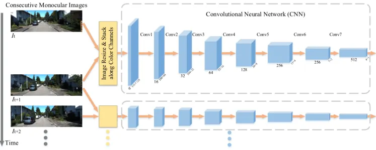
FIGURE 2. Architecture of the convolutional neural network with input images.
and fine-tuned. In contrast, our method adopts an end-to-end training framework and requires less engineering effort.
B. DEEP LEARNING BASED VO SYSTEM
In recent years, deep neural networks have been widely used in the robotics and computer vision domain and have shown remarkable robustness in challenging environments [30]. This is due to the more descriptive features extracted and the extremely large and diverse data used for training. PoseNet proposed by Kendallet al.[3] shows the first implementation on pose estimation, which directly generates the six degrees of freedom (6-DoF) of a camera from a single RGB input image. The model GoogLeNet pre-trained on other classifica-tion tasks is leveraged for pose regression [31]. The softmax layers that originally output classification results are removed and replaced by a seven-dimensional pose vector. The last fully connected layers are also modified.
Since CNNs extracts more robust features than traditional feature detectors, the system can achieve a high accuracy even under some extreme conditions, such as intense lighting and blur images. PoseNet can also be easily generalized to other scenes through transfer learning technique. The model on the new task can thus be trained with smaller dataset and shorter time. Liet al.[5] incorporated another CNN stream to PoseNet and fed depth images into this stream to enhance the re-localization accuracy. ORB-SLAM is used to label the collected images as ground truth. However, all of these deep learning based methods require ground truth for training, which can be quite expensive and labor-intensive.
Attentions have been recently drawn to the unsupervised field due to the shortcomings of the aforementioned super-vised methods. Zhou et al.[13] presented an unsupervised deep learning framework for depth and camera motion esti-mation. Their depth prediction and the pose estimation results
were promising. However, this method failed to recovery absolute scale due to the limitation caused by using monoc-ular images only. A scale factor needs to be calculated from ground truth each time when a pose is estimated and the value of the scale factor is non-constant.
RCNNs were first introduced by Liang and Hu [32] and Renet al.[33] for object recognition and detection, respec-tively. Donahue et al. [34] also proposed a RCNN model for activity recognition, image and video description tasks. All of these works use video as input data. Wanget al.[4] first employed a RCNN for pose estimation, which however needs ground truth poses for training. In contrast, this paper is focused on the unsupervised aspect, following our previous work [14]. Instead of stereo vision, we use data from a monocular camera and a LiDAR for training.
III. THE PROPOSED APPROACH
In this section, we discuss the proposed VO system in detail. The network architecture is given first. The loss functions used to penalize the system output are subsequently intro-duced. Finally, the implementations of the network and loss functions are presented.
A. SYSTEM ARCHITECTURE
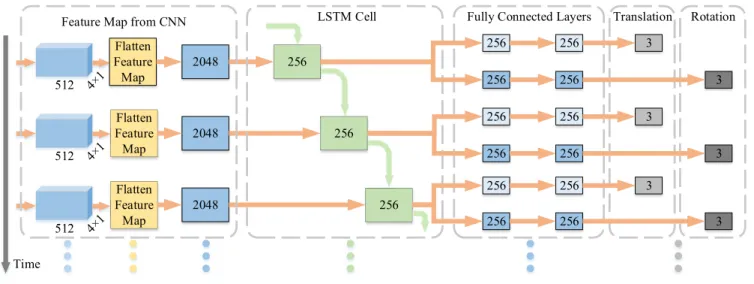
The proposed RCNN is presented in Fig.2and Fig.3. More specifically, Fig. 2 shows the architecture of the Convolu-tional Neural Network, which can be viewed as a feature extractor. We take two consecutive monocular images each time and feed them into the network for training. The images are resized to 416×128×3 and then stacked along color chan-nels.Convrepresents convolutional layers. The blue cubes represent feature maps with shapes under them. Fig.3shows the architecture of the Recurrent Neural Network, which can be viewed as a pose estimator. The network takes the last
FIGURE 3. Architecture of the recurrent neural network with output poses.
TABLE 1. Specifics of the convolutional layers.
feature maps from the CNN and directly outputs translation and rotation matrices. The numbers in blue and gray boxes represent the size of vectors.
The number of hidden units in a LSTM cell was selected arbitrarily or empirically in past works [4], [14], [34]. Since our training dataset is relatively small, we decrease the value to 256 to avoid over-fitting. The CNN takes two raw RGB images as input and generates a feature map. The feature map is then fed into the RNN which finally generates a transformation matrix between the input images.
It becomes clear that CNNs that are originally trained for a specific task can be modified and reused for other related but different tasks [35], [36] since the generic features learned by a model, especially from lower convolutional layers, are versatile and transferable [30]. Recently, several models have been proposed and shown promising performance such as AlexNet [37], GoogLeNet [31] and ResNet [38]. Our CNN is based on the network originates from Visual Geometry Group neural network (VGG) [39]. Table1lists the specifics of each modified convolutional layer.
Fig. 2 uses KITTI dataset as an example input. The CNN model can be regarded as an image feature extractor and descriptor. Assume thatI1,I2, ...,It, ...,INare a sequence
of monocular images used for training. The CNN takes every two consecutive images as input and yieldsN−1 feature maps with the size of which are 4×1×512. The input images are first resized to 416×128×3, stacked along color channels and then fed into the network. There are 7 convolutional layers in the CNN.
We use stride 2 to regulate the movement of all of the convolutional filters (receptive field or kernel) for pixel-wise operations across image space. This leads to lower output volume. Since neighboring pixels are strongly correlated in lower layers, the sizes of the filters in the first two convolu-tional layers are 7×7 and 5×5, respectively. The size drops to 3×3 for the rest layers to capture fine details. The zero-padding decreases along with the kernel size from 3 to 2 and then 1 so that the spatial dimension of the input volume can be preserved.
Each convolutional layer is followed by a Rectified Linear Unit (ReLU) nonlinear activation function. Batch normal-ization, which is a commonly used technique for improving performance of neural networks is not employed in our CNN. Instead, it results in slow and unstable loss convergence in our experiments. One possible reason is because batch nor-malization normalizes the input layer by adjusting and scal-ing the activations. The absolute differences between image pixels or features are ignored and only relative differences are taken into consideration. In this way, batch normalization can reduce the training difficulty for classification tasks since it can retain the structure of an image while highlighting the inconspicuous regions. However, the contrast information of an image needs to be preserved rather than stretched for VO tasks. Thus, batch normalization is not applied in our system.
The feature maps generated from the CNN are reshaped and flattened toN−1 chronological vectors. The RNN takes these vectors as input and learns connections in the sequence
of image. However, in practice, it is difficult to train a stan-dard RNN to solve problems that require learning long-term temporal dependencies, since the gradient of the loss function decays exponentially with time until vanishes or explodes. Thus, we adopt a popular solution by incorporating Long Short-Term Memory (LSTM) units [40] into the RNN.
Compared to standard RNNs, LSTM networks introduce three gates, namely input, forget and output gates, which allow for a better control over the gradient flow and preser-vation of long-term temporal dependencies. The key to an LSTM network is updating the cell state through time, which is represented by the green arrows in Fig. 3. Only one LSTM layer is applied in the RNN. We follow Kawakami’s suggestion [41] and set the biases of the forget gate to 1 to reduce the scale of forgetting at the beginning of training. The projection layer is not used in the LSTM cell, thus the dimension of the output is also 256.
The output vectors from the RNN represents high-level features of the transformation information between two con-secutive frames. We then follow the idea proposed in [4] and feed them into two fully connected layers to learn nonlinear combinations of these features. The fully connected layers have connections to all activations in the previous layer, thus can realize high-level meaningful reasoning. Unlike other deep learning based methods which output a single vector representing 6-DoF, two parallel streams are introduced in our system to infer translation and rotation independently. This is due to the fact that rotation is highly nonlinear and always harder to be trained.
A traditional solution based on practical experience is by raising the weight of rotation loss. We further extend this idea and use two separate streams to collect different features for estimation. The dimension of the fully connected layers is 256 which is the same as the output dimension of the LSTM. Each layer is followed by a Exponential Linear Unit (ELU) activation function. Finally, the translation and rotation (rep-resented by Euler angles) vectors are generated and used for back-propagation.
B. LOSS FUNCTIONS
In this section, we introduce how the loss functions are designed in our system. The loss functions or cost functions describe how far off the pose our RCNN produced is from the expected result. The loss indicates the magnitude of error our model made on its inaccurate prediction. We minimize the loss in order to make the output of the network closer to the truth. In our system, the total loss consists of 2D and 3D spatial losses. The loss is calculated by using transforma-tion matrices generated by our RCNN and pairs of consecu-tive monocular images and point clouds.
Assume that I1,I2, ...,It,It+1, ...,IN is a sequence of
monocular images in chronological order used for training and D1,D2, ...,Dt,Dt+1, ...,DN are the associated depth
images. It and It+1,(1 ≤ t < t + 1 ≤ N) are two
consecutive frames in this image sequence. To compute 2D spatial loss, we first project a point from It to It+1
using the transformation matrix and its depth value. A new frameIˆt can then be reconstructed from the projected point
inIt+1. Finally, we compareIˆt withIt for loss calculation.
In terms of 3D spatial loss, we directly swap a point cloud to its neighboring frame through the transformation matrix and compare their difference.
1) 2D SPATIAL LOSS
Pairs of consecutive RGB images and point clouds are used to compute 2D spatial loss. We first rescale the voxel values of the point clouds to 0-255 and project the point clouds to single-channel 2D depth images. Thus, each pixel in a calibrated depth image represents the depth value of the corresponding point in the associated monocular image.
Let pt(ut,vt) and dt denote a point in It and its depth
value inDt, respectively. We then try to project pt to the
frame It+1 at time t + 1. Assume the projected point in It+1ispˆt+1(uˆt+1,vˆt+1). Based on the pinhole camera model,
a scene view can be formed by projecting 3D points in the world coordinate system into the image 2D plane using a perspective transformation dtpt =KPt (1) or dt ut vt 1 =K xt yt zt , (2)
whereK is the camera intrinsic matrix, Pt(xt,yt,zt) is the
voxel in the world coordinate system projected from pointpt.
Note that in Equation2,dt =zt.
On the other hand, based on 3D linear transformation theory, we have ˆ Pt+1= ˆRt−>t+1Pt+ ˆtt−>t+1 (3) or ˆ Pt+1= ˆRt−>t+1dtK−1pt + ˆtt−>t+1, (4)
where Pˆt+1 is the voxel in the world coordinate system
projected frompˆt+1.Rˆt−>t+1(converted from Euler angles)
and ˆtt−>t+1 are the rotation matrix and translation vector
generated by the RCNN, respectively. The size of rotation matrixRˆt−>t+1is 3×3, whereas the size of translation vector ˆ
tt−>t+1is 3×1. We can then projectPˆt+1(xˆt+1,yˆt+1,zˆt+1)
to the image 2D plane through
ˆ dt+1 ˆ ut+1 ˆ vt+1 1 =K ˆ xt+1 ˆ yt+1 ˆ zt+1 , (5)
wheredˆt+1is the depth value ofpˆt+1(uˆt+1,vˆt+1) anddˆt+1= ˆ
zt+1. In this way, we can derivepˆt+1frompt by ˆ pt+1= 1 ˆ zt+1 K(Rˆt−>t+1dtK−1pt+ ˆtt−>t+1). (6)
We then use the framework proposed by Jaderberg et al. [42] to reconstruct It. More specifically,
the value ofpt in the reconstructed imageIˆt is generated by
the top left, top right, bottom left and bottom right neighbors ofpˆt+1inIt+1. Similarly, we can reconstruct imageIt+1by
ˆ pt = 1 ˆ zt K(Rˆt+1−>tdt+1K−1pt+1+ ˆtt+1−>t), (7)
wherept+1is a point inIt+1,pˆt is the projected point in It, dt+1is the depth value ofpt+1,Pˆt(xˆt,ˆyt,zˆt) is the voxel in
the world coordinate system projected frompˆt,Rˆt+1−>t = ˆ
R−t−1>t+1,ˆtt+1−>t = − ˆR−t−1>t+1ˆtt+1−>t.
Finally, the 2D spatial loss can be represented by
L2D= N−1 X t=1 |It− ˆIt| + |It+1− ˆIt+1| . (8) 2) 3D SPATIAL LOSS
3D spatial loss is computed by using point clouds and trans-formation matrices generated from the RCNN. AssumeCt
andCt+1,(1 ≤ t < t+1 ≤ N) are two consecutive point
clouds which are inverse-projected fromDt andDt+1to the
world coordinate system. Letctdenote a point inCt, we then
project this point to Ct+1 through transformation matrix.
Based on 3D linear transformation theory, the projected point can be derived by
ˆ
ct+1= ˆRt−>t+1ct+ ˆtt−>t+1. (9)
The reconstructed point cloudCˆt+1can thus be obtained.
We can also reconstructCˆtfromCt+1by ˆ
ct = ˆRt+1−>tct+1+ ˆtt+1−>t, (10)
wherect+1is a point inCt+1 andcˆt is the projected point
inCˆt.
Finally, we employ a strategy similar to Iterative Closest Point (ICP) algorithm proposed by Chen and Medioni [43] for 3D spatial loss calculation. Similar strategy is also adopted by Mahjourianet al.[44]. L3D= N−1 X t=1 |Ct− ˆCt| + |Ct+1− ˆCt+1| . (11) The total loss can thus be acquired by
L =λ2DL2D+λ3DL3D, (12)
whereλ2D andλ3D are the weights for 2D and 3D spatial
losses, respectively. C. IMPLEMENTATION
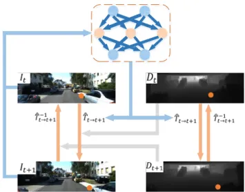
Fig.4presents an overview of the network and loss function implementations and how back-propagation operates in the proposed RCNN. In the figure, we use two pairs of consecu-tive monocular and depth images for illustration. No ground truth poses are used for training. The transformation matrix generated from the network is used for loss calculation. The transformation matrix Tˆt−>t+1 directly generated from the
network and its inverseTˆt−−1>t+1are used for loss calculation.
FIGURE 4. Overview of the training process.
Specifically, we use the monocular imageIt, depth
infor-mationDt at timet and the transformation matrixTˆt−>t+1
to reconstruct the monocular imageIˆt+1at timet+1.
Sim-ilarly, the reconstructed monocular image Iˆt at time t can
be obtained by the monocular imageIt+1, depth information Dt+1 at time t + 1 and the inverse of the transformation
matrixTˆt−−1>t+1. The 2D spatial lossL2Dcan thus be
calcu-lated by Equation8. We then use the depth informationDt at
timetand the transformation matrixTˆt−>t+1to reconstruct
the depth informationDˆt+1at timet+1.
Similarly, the depth information Dˆ
t at time t can be
obtained by the depth informationDt+1at timet+1 and the
inverse of the transformation matrixTˆt−−1>t+1. The 3D spatial loss L3D can thus be calculated by Equation 11. We then
calculate the total loss L based on Equation 12. The total loss is then back propagated through the network, adjusting its weights and making it closer to the truth in the next round. The orange arrows show how a pixel or a voxel can be projected to its neighboring frame. Depth images are used for both 2D and 3D spatial loss calculation, thus the abso-lute scale can be recovered. Algorithm1presents a detailed implementation scheme.
IV. EXPERIMENTS
In this section, we first present the training details and then compare the performance of our VO system with other state-of-the-art algorithms in terms of both translation and rotation accuracy.
A. TRAINING
We trained the proposed RCNN on a DELL workstation with an Intel Core i7-4790K @4.0GHz CPU and a Nvidia GeForce GTX Titan X 12GB Memory GPU. The model implemen-tation environment is TensorFlow [45], which is an open source software library originating from Google’s Machine Intelligence research organization for numerical computation using data flow graphs. For fair comparison in SectionIV-B,
Algorithm 1 Implementations of the RCNN and Loss Functions
Input : Consecutive monocular images{I1,I2, ...,IN}
Associated depth images{D1,D2, ...,DN}
Output: Trained RCNN functionprepare_Training_Data
fori in(1:N+1)do
ifi>(Nseq−1)/2and i<N−(Nseq−1)/2
then
resizeIito 416×128×3;
project Velodyne point cloud to depth image
Di;
resizeDito 416×128×1;
stackIiandDihorizontally;
save camera intrinsics matrix file; end
end
split data into two parts for training and testing; end
functionbuild_Training_Graph
prepare training data and camera intrinsics matrix path;
design data augmentation based on luminanceγ, scalesx,syand rotationrd;
design the RCNN;
design total lossL =λ2DL2D+λ3DL3D;
end
functionTrain
load hyper parameters;
setthres_Epoch=30 based on experimental experience;
ifepoch<thres_Epochthen
feed training data into the RCNN; computeL;
adjust the RCNN parameters; ifstep%500=0then collect summary; save network; end else break end end
we adopted the same training dataset presented by Zhouet al.[13] based on KITTI dataset only.
Before training, we resized the monocular images to 416 ×128 with 3 RGB channels and projected associated 3D point clouds to 2D single-channel depth images. Each point in a depth image represents the depth value of the cor-responding point in the monocular image. Since KITTI data is relatively limited, online data augmentation technique is applied to enlarge the dataset and the results are shown in Fig. 5. More specifically, the augmentation processing includes:
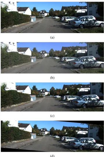
FIGURE 5. Data augmentation. (a) Original monocular image without data augmentation. (b) Luminance correction. (c) Image rescale and cropping. (d) Clockwise image rotation.
• Luminance: The input monocular images are randomly corrected by gammaγ ∈[0.7,1.3].
• Scale: The input monocular and depth images are ran-domly scaled by scale factors sx ∈ [1,1.2] andsy ∈
[1.0,1.2] along X-axis and Y-axis, respectively. The images are then randomly cropped to 416×128.
• Rotation: The input monocular and depth images are
randomly rotated by r ∈ [−5,5] degrees. Nearest-neighbor interpolation is used.
Note that the camera equipped on the KITTI car has a wider field-of-view than the LiDAR sensor, thus we only used the cropped region presented in [46] for loss calculation, as shown in Fig.6.
We then fed pairs of monocular and depth images into the RCNN and trained the network from scratch. No ground truth poses were used during training. We employed the Adam optimization algorithm [47], which is an extension to Stochastic Gradient Descent (SGD) method and has recently been widely adopted in deep learning. We followed their idea and set the exponential decay rates for the first and second moment estimatesβ1 = 0.9 andβ2 = 0.999, respectively.
FIGURE 6. Region of interest for loss calculation. Ignored region is grayed out. X-axis: from 15 to 401. Y-axis: from 53 to 126.
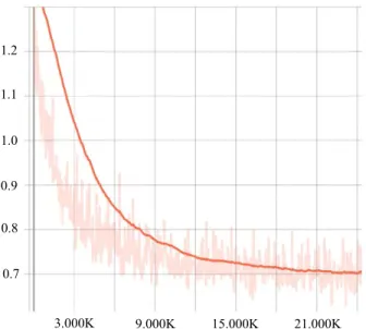
FIGURE 7. Training loss. X-axis: training steps. Y-axis: total loss.
We set N = 5 and trained the RCNN for 40 epochs in total. The batch size is 32. Our learning rate schedule is step-decay based. The initial learning rate was set to 0.0002 and dropped to 0.0001 after 3/4 of the total training steps to allow more fine-grained weight updates. No batch normalization was used since we found that it resulted in slow and unstable loss convergence in our experiments.
The total loss against training steps is shown in Fig.7. The noisy light line represents the raw data of the total loss and the dark line is the smoothing result of the total loss. The smoothing algorithm we use is a moving average. Given a pointplossat stepsp, it replacesplosswith an average of the
points in the range of [sp −5000,sp +5000]. The range
is reduced on both sides ofsp to fit exactly the number of
elements available if there are less than 5,000 steps to the left. This means that the smoothed value is higher than its true value and gradually becomes close to its true value until the desired range is reached. We have removed the data after step 24,000 since the smoothed total loss remains almost constant. As can be seen from Fig.7, the total loss dropped rapidly before 9,000 steps and then reduced slowly. Finally, it reached 0.7 at step 24,000.
At the same time, the disparity image between a monocular image and its projected image were used to visualize and monitor the training process. Fig.8(a) shows the disparity at the beginning of training and Fig. 8(b) shows the disparity
FIGURE 8. Change of disparity during training. (a) Disparity at the beginning of training. (b) Disparity at the end of training.
at the end of training. It is clear that the images grew darker during training, i.e., the disparity was narrowed.
B. PERFORMANCE EVALUATION
Performance evaluation was carried out on a desktop with an Intel Core i7-3370 @3.4GHz CPU and a Nvidia GeForce GTX 980 4GB Memory GPU. Our proposed VO system was compared with other state-of-the-art VO systems based on KITTI Odometry dataset. The benchmark includes 22 stereo sequences and ground truth poses are provided for 00-10 sequences. The images were captured on a vehicle at 10 Hz which was moving in a city, rural areas and on highways at speed ranging from 0 km/h to 90 km/h. The scenes in the dataset are not static. Moving objects include cars and pedestrians. All these factors produce disturbance to VO systems and make the task more challenging.
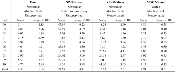
Our system can generate VO on an absolute scale without data post-processing. During testing, the network took only consecutive monocular images as input and directly gener-ated poses. Thus our system is still a monocular VO sys-tem. We compare the proposed method to other state-of-the-art monocular VO systems, namely SfMLearner [13], VISO2-Mono. VISO2-Stereo [48] which is a stereo VO sys-tem is also used as a reference. No loop-closure detection (automatic or manual tagging) was applied and the same parameter set was used for all sequences.
Our system and SfMLearning are unsupervised deep learn-ing based, whereas VISO2-Mono and VISO2-Stereo are feature based. Since SfMLearning relies on ground truth poses for scale recovery, we post-processed the SfMLearn-ing results for comparison. VISO2-Mono recovers absolute scale through a fixed camera height. VISO2-Stereo directly outputs poses on an absolute scale since it employs stereo sequences for testing. The input image resolution of our system and SfMLearning is 416×128, whereas VISO2-Mono and VISO2-Stereo adopt a 1242×376 setting.
Fig. 9 shows the trajectories of KITTI Odometry from Sequence 02 to Sequence 10. The results were generated by our system, SfMLearner and VISO2-Mono. Ground truth trajectories are provided as a reference. Sequence 01 is omit-ted since the sequence was captured on a highway with
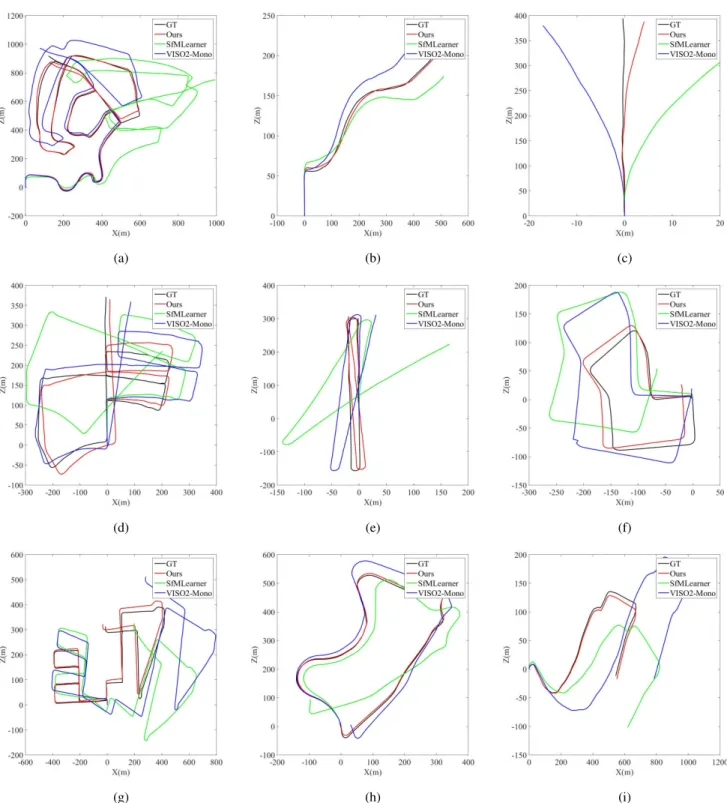
FIGURE 9. Trajectories of KITTI Odometry sequence 02-10 which are produced by our system, SfMLearner and VISO2-Mono. Ground truth trajectories are provided as a reference. SfMLearner results are post-processed with ground truth poses for scale recovery. Only 2D trajectories (X-axis and Z-axis) are provided for clearer presentation. The vertical Y-axis is omitted. Note that Sequence 09 and 10 are not used for training. (a) Sequence 02. (b) Sequence 03. (c) Sequence 04. (d) Sequence 05. (e) Sequence 06. (f) Sequence 07. (g) Sequence 08. (h) Sequence 09. (i) Sequence 10.
rare features. Thus, all methods including VISO2-Stereo failed to recover the absolute scale. As can be seen from Fig. 9, the proposed method outperforms other monocular VO systems. The generated trajectories are the closest to the ground truth ones. It should be noticed that Sequence 09
and 10 are not used for training. However, the results of these two sequences show the pre-trained model can be generalized and applied to other similar scenes.
The detailed translational and rotational errors are listed in Table 2. We adopt Root Mean Square Error (RMSE)
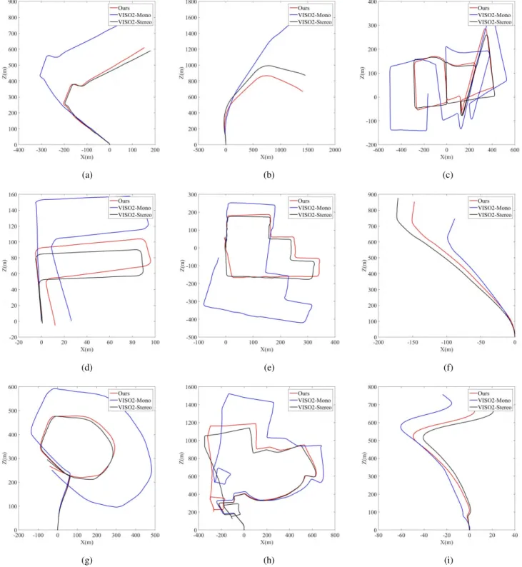
FIGURE 10. Trajectories of KITTI Odometry sequence 11-15 and 17-20 which are produced by our system and VISO2-Mono. VISO2-Stereo trajectories are provided as a reference. No ground truth poses are provided for these sequences. Only 2D trajectories (X-axis and Z-axis) are provided for clearer presentation. The vertical Y-axis is omitted. (a) Sequence 11. (b) Sequence 12. (c) Sequence 13. (d) Sequence 14. (e) Sequence 15. (f) Sequence 17. (g) Sequence 18. (h) Sequence 19. (i) Sequence 20.
recommended by KITTI for evaluation. The translational errors are measured in percent (%), whereas the rotational errors are measured in degrees per meter (◦/m). Each value in the table was obtained by averaging errors of all possible subsequences of length 100, 200,..., 800 meters. From the
table we can see our method generated lower errors than other monocular systems in terms of both translation and rotation and can be compared to a stereo VO system. We can further reduce the rotational errors by manually increasing the ratio of the training images captured when the vehicle is turning.
TABLE 2. Translational and rotational errors. VISO2-Stereo results are provided as a reference. SfMLearner poses are post-processed with ground truth poses for scale recovery. Sequence 09 and 10 are not used for training.
Since KITTI dataset is relatively small, the overall perfor-mance of our network can also be improved by employing larger dataset for training.
The trajectories of KITTI Odometry from Sequence 11 to 15 and from Sequence 17 to 20 are presented in Fig. 10. VISO2-Stereo trajectories are also provided as a reference. No ground truth poses are provided for these sequences. Thus, quantitative evaluation cannot be carried out. We can see the performance of our method is close to VISO2-Stereo (our tra-jectories are closer to VISO2-Stereo than VISO2-Mono). The deviations of the estimated rotation and translation matrices inevitably exist due to significant speed changes and sharp turns. In addition, in the case when the car bumps, the distance from the camera to the ground changes. Therefore, using a fixed value to recover absolute scale is not reliable. From the figures we can tell our method generally outperforms VISO2-Mono in terms of translation estimation (Figure 10a, 10d, 10e, 10f, 10g) and rotation estimation (Figure 10b, 10c, 10h).
Although the proposed method outperforms other monoc-ular VO systems in terms of translation and rotation accuracy, the processing time is longer. We set batch size to 1 for pose generation. The processing time is 0.09 second per pose based on a Nvidia GeForce GTX 980 GPU and the input image size being 416 ×128 ×3, whereas Mono and VISO2-Stereo systems require only a CPU to achieve a similar speed. Compared to other deep learning based methods, we require no ground truth poses for training or scale post-processing, but still need depth information for injecting the scale.
V. CONCLUSION
This paper proposed a monocular visual odometry sys-tem based on deep learning technique. The syssys-tem oper-ates in an unsupervised end-to-end training manner.
Consecutive monocular images and depth information are used for training. As no ground truth pose labeling is needed, the proposed system requires less human effort and is cheap to run. For testing, the proposed system takes only monocular images as input and directly generates poses on an absolute scale. Experiments were carried out on KITTI dataset. Results have shown that our system outper-forms other monocular VO systems in terms of translation and rotation accuracy and can be compared to stereo VO sys-tems. The pre-trained model can also be generalized to other scenes. The performance of the system can be improved by further training.
The proposed method requires high computing power and is difficult to achieve real-time performance. In the future, we will continue improving its computing efficiency based on the unsupervised training manner. Depth information will be incorporated during testing in order to boost system per-formance for real-time navigation of autonomous robots and the visual guidance of blind people.
ACKNOWLEDGMENTS
The authors would like to thank Robin Dowling and Ian Dukes for their technical support.
CONFLICT OF INTEREST
The authors declare that they have no conflict of interest. REFERENCES
[1] F. Fraundorfer and D. Scaramuzza, ‘‘Visual odometry: Part II: Matching, robustness, optimization, and applications,’’IEEE Robot. Autom. Mag., vol. 19, no. 2, pp. 78–90, Jun. 2012.
[2] S. Wang, R. Clark, H. Wen, and N. Trigoni, ‘‘DeepVO: Towards end-to-end visual odometry with deep recurrent convolutional neural net-works,’’ inProc. IEEE Int. Conf. Robot. Autom. (ICRA), May/Jun. 2017, pp. 2043–2050.
[3] A. Kendall, M. Grimes, and R. Cipolla, ‘‘PoseNet: A convolutional net-work for real-time 6-DOF camera relocalization,’’ inProc. IEEE Int. Conf. Comput. Vis. (ICCV), Dec. 2015, pp. 2938–2946.
[4] S. Wang, R. Clark, H. Wen, and N. Trigoni, ‘‘End-to-end, sequence-to-sequence probabilistic visual odometry through deep neural networks,’’ Int. J. Robot. Res., vol. 37, nos. 4–5, p. 0278364917734298, 2017. [5] R. Li, Q. Liu, J. Gui, D. Gu, and H. Hu, ‘‘Indoor relocalization in
challeng-ing environments with dual-stream convolutional neural networks,’’IEEE Trans. Autom. Sci. Eng., vol. 15, no. 2, pp. 651–662, Apr. 2018. [6] A. Kendall and R. Cipolla, ‘‘Geometric loss functions for camera pose
regression with deep learning,’’ inProc. IEEE Conf. Comput. Vis. Pattern Recognit. (CVPR), Jul. 2017, pp. 6555–6564.
[7] P. Henry, M. Krainin, E. Herbst, X. Ren, and D. Fox, ‘‘RGB-D mapping: Using depth cameras for dense 3D modeling of indoor environments,’’ inProc. 12th Int. Symp. Exp. Robot. (ISER). Berlin, Germany: Springer, Dec. 2010, pp. 477–491.
[8] F. Steinbrücker, J. Sturm, and D. Cremers, ‘‘Real-time visual odometry from dense RGB-D images,’’ inProc. IEEE Int. Conf. Comput. Vis. Work-shops (ICCV WorkWork-shops), Nov. 2011, pp. 719–722.
[9] A. S. Huanget al., ‘‘Visual odometry and mapping for autonomous flight using an RGB-D camera,’’ inRobotics Research. Cham, Switzerland: Springer, 2017, pp. 235–252.
[10] J. Engel, J. Stückler, and D. Cremers, ‘‘Large-scale direct SLAM with stereo cameras,’’ inProc. IEEE/RSJ Int. Conf. Intell. Robots Syst. (IROS), Sep./Oct. 2015, pp. 1935–1942.
[11] R. Wang, M. Schwörer, and D. Cremers, ‘‘Stereo DSO: Large-scale direct sparse visual odometry with stereo cameras,’’ inProc. IEEE Int. Conf. Comput. Vis. (ICCV), Oct. 2017, pp. 3903–3911.
[12] J. Zhang and S. Singh, ‘‘Visual-lidar odometry and mapping: Low-drift, robust, and fast,’’ inProc. IEEE Int. Conf. Robot. Autom. (ICRA), May 2015, pp. 2174–2181.
[13] T. Zhou, M. Brown, N. Snavely, and D. G. Lowe, ‘‘Unsupervised learning of depth and ego-motion from video,’’ inProc. IEEE Conf. Comput. Vis. Pattern Recognit. (CVPR), Jul. 2017, pp. 6612–6619.
[14] R. Li, S. Wang, Z. Long, and D. Gu, ‘‘UnDeepVO: Monocular visual odometry through unsupervised deep learning,’’ inProc. IEEE Int. Conf. Robot. Autom. (ICRA), May 2018, pp. 7286–7291.
[15] A. Geiger, P. Lenz, C. Stiller, and R. Urtasun, ‘‘Vision meets robotics: The KITTI dataset,’’Int. J. Robot. Res., vol. 32, no. 11, pp. 1231–1237, 2013. [16] D. Nistér, O. Naroditsky, and J. Bergen, ‘‘Visual odometry,’’ in Proc.
IEEE Comput. Soc. Conf. Comput. Vis. Pattern Recognit., vol. 1, Jun./Jul. 2004, pp. 1–8.
[17] A. Howard, ‘‘Real-time stereo visual odometry for autonomous ground vehicles,’’ in Proc. IEEE/RSJ Int. Conf. Intell. Robots Syst. (IROS), Sep. 2008, pp. 3946–3952.
[18] P. Corke, D. Strelow, and S. Singh, ‘‘Omnidirectional visual odometry for a planetary rover,’’ inProc. IEEE/RSJ Int. Conf. Intell. Robots Syst. (IROS), vol. 4, Sep. 2004, pp. 4007–4012.
[19] P. Henry, M. Krainin, E. Herbst, X. Ren, and D. Fox, ‘‘RGB-D mapping: Using Kinect-style depth cameras for dense 3D modeling of indoor environments,’’Int. J. Robot. Res., vol. 31, no. 5, pp. 647–663, 2012. [20] L. Kneip, M. Chli, and R. Y. Siegwart, ‘‘Robust real-time visual odometry
with a single camera and an IMU,’’ inProc. Brit. Mach. Vis. Conf., 2011, pp. 1–12.
[21] B. Kitt, A. Geiger, and H. Lategahn, ‘‘Visual odometry based on stereo image sequences with RANSAC-based outlier rejection scheme,’’ inProc. IEEE Intell. Vehicles Symp., Jun. 2010, pp. 486–492.
[22] T. D. Barfoot, ‘‘Online visual motion estimation using FastSLAM with SIFT features,’’ inProc. IEEE/RSJ Int. Conf. Intell. Robots Syst. (IROS), Aug. 2005, pp. 579–585.
[23] R. Mur-Artal, J. M. M. Montiel, and J. D. Tardós, ‘‘ORB-SLAM: A versatile and accurate monocular SLAM system,’’IEEE Trans. Robot., vol. 31, no. 5, pp. 1147–1163, Oct. 2015.
[24] R. Mur-Artal and J. D. Tardós, ‘‘ORB-SLAM2: An open-source slam system for monocular, stereo, and RGB-D cameras,’’IEEE Trans. Robot., vol. 33, no. 5, pp. 1255–1262, Oct. 2017.
[25] G. Klein and D. Murray, ‘‘Parallel tracking and mapping for small AR workspaces,’’ in Proc. 6th IEEE ACM Int. Symp. Mixed Augmented Reality, Nov. 2007, pp. 225–234.
[26] R. A. Newcombeet al., ‘‘KinectFusion: Real-time dense surface mapping and tracking,’’ inProc. IEEE Int. Symp. Mixed Augmented Real. (ISMAR), Oct. 2011, pp. 127–136.
[27] R. A. Newcombe, S. J. Lovegrove, and A. J. Davison, ‘‘DTAM: Dense tracking and mapping in real-time,’’ inProc. IEEE Int. Conf. Comput. Vis. (ICCV), Nov. 2011, pp. 2320–2327.
[28] J. Engel, J. Sturm, and D. Cremers, ‘‘Semi-dense visual odometry for a monocular camera,’’ inProc. IEEE Int. Conf. Comput. Vis. (ICCV), Dec. 2013, pp. 1449–1456.
[29] J. Engel, T. Schöps, and D. Cremers, ‘‘LSD-SLAM: Large-scale direct monocular SLAM,’’ inProc. Eur. Conf. Comput. Vis.Cham, Switzerland: Springer, 2014, pp. 834–849.
[30] N. Sünderhauf, S. Shirazi, F. Dayoub, B. Upcroft, and M. Milford, ‘‘On the performance of ConvNet features for place recognition,’’ in Proc. IEEE/RSJ Int. Conf. Intell. Robots Syst. (IROS), Sep./Oct. 2015, pp. 4297–4304.
[31] C. Szegedyet al., ‘‘Going deeper with convolutions,’’ inProc. IEEE Conf. Comput. Vis. Pattern Recognit. (CVPR), Jun. 2015, pp. 1–9.
[32] M. Liang and X. Hu, ‘‘Recurrent convolutional neural network for object recognition,’’ inProc. IEEE Conf. Comput. Vis. Pattern Recognit. (CVPR), Jun. 2015, pp. 3367–3375.
[33] S. Ren, K. He, R. Girshick, and J. Sun, ‘‘Faster R-CNN: Towards real-time object detection with region proposal networks,’’ inProc. Adv. Neural Inf. Process. Syst., 2015, pp. 91–99.
[34] J. Donahueet al., ‘‘Long-term recurrent convolutional networks for visual recognition and description,’’ inProc. IEEE Conf. Comput. Vis. Pattern Recognit. (CVPR), Jun. 2015, pp. 2625–2634.
[35] P. Ren, W. Sun, C. Luo, and A. Hussain, ‘‘Clustering-oriented multiple convolutional neural networks for single image super-resolution,’’Cogn. Comput., vol. 10, no. 1, pp. 165–178, 2017.
[36] M. Oquab, L. Bottou, I. Laptev, and J. Sivic, ‘‘Learning and transferring mid-level image representations using convolutional neural networks,’’ inProc. IEEE Conf. Comput. Vis. Pattern Recognit. (CVPR), Jun. 2014, pp. 1717–1724.
[37] A. Krizhevsky, I. Sutskever, and G. E. Hinton, ‘‘ImageNet classification with deep convolutional neural networks,’’ in Proc. Adv. Neural Inf. Process. Syst., 2012, pp. 1097–1105.
[38] K. He, X. Zhang, S. Ren, and J. Sun, ‘‘Deep residual learning for image recognition,’’ inProc. IEEE Conf. Comput. Vis. Pattern Recognit. (CVPR), Jun. 2016, pp. 770–778.
[39] K. Simonyan and A. Zisserman. (2014). ‘‘Very deep convolutional networks for large-scale image recognition.’’ [Online]. Available: https://arxiv.org/abs/1409.1556
[40] S. Hochreiter and J. Schmidhuber, ‘‘Long short-term memory,’’Neural Comput., vol. 9, no. 8, pp. 1735–1780, 1997.
[41] K. Kawakami, ‘‘Supervised sequence labelling with recurrent neural networks,’’ Ph.D. dissertation, Dept. Lang. Technol. Inst., Tech. Univ. Munich, Munich, Germany, 2008.
[42] M. Jaderberg, K. Simonyan, A. Zisserman, and K. Kavukcuoglu, ‘‘Spatial transformer networks,’’ inProc. Adv. Neural Inf. Process. Syst., 2015, pp. 2017–2025.
[43] Y. Chen and G. Medioni, ‘‘Object modelling by registration of multiple range images,’’Image Vis. Comput., vol. 10, no. 3, pp. 145–155, Apr. 1992. [44] R. Mahjourian, M. Wicke, and A. Angelova, ‘‘Unsupervised learning of depth and ego-motion from monocular video using 3D geometric constraints,’’ inProc. IEEE Conf. Comput. Vis. Pattern Recognit. (CVPR), Jun. 2018, pp. 5667–5675.
[45] TensorFlow. Accessed: May 29, 2018. [Online]. Available: https://www. tensorflow.org/
[46] D. Eigen, C. Puhrsch, and R. Fergus, ‘‘Depth map prediction from a single image using a multi-scale deep network,’’ inProc. Adv. Neural Inf. Process. Syst., 2014, pp. 2366–2374.
[47] D. P. Kingma and J. Ba. (2014). ‘‘Adam: A method for stochastic optimization.’’ [Online]. Available: https://arxiv.org/abs/1412.6980 [48] A. Geiger, J. Ziegler, and C. Stiller, ‘‘StereoScan: Dense 3D reconstruction
in real-time,’’ in Proc. IEEE Intell. Vehicles Symp. (IV), Jun. 2011, pp. 963–968.
QIANG LIU received the B.Eng. and M.Eng. degrees in automation and control engineering from the Harbin Institute of Technology, Harbin, China, in 2012 and 2014, respectively, and the Ph.D. degree in computer science from the Uni-versity of Essex, Colchester, U.K., in 2019. His research interests include robotics, deep learning, semantic mapping and localization, and place and object recognition.
RUIHAO LIreceived the B.Sc. degree in automa-tion from the Beijing Institute of Technology, Beijing, China, in 2012, the M.Sc. degree in con-trol science and engineering from the National University of Defense Technology, Changsha, China, in 2014, and the Ph.D. degree in robotics from the University of Essex, U.K. His research interests include robotics, SLAM, deep learning, and semantic scene understanding.
HUOSHENG HU (M’94–SM’01) received the M.Sc. degree in industrial automation from Cen-tral South University, China, in 1982, and the Ph.D. degree in robotics from the University of Oxford, U.K., in 1993. He is currently a Pro-fessor with the School of Computer Science and Electronic Engineering, University of Essex, U.K., leading the Robotics Research Group. His research interests include behavior-based robotics, human– robot interaction, embedded systems, multi-sensor data fusion, machine learning algorithms, mechatronics, pervasive comput-ing, and service robots. He has authored over 500 papers in journals, books, and conferences in these areas. He is a fellow of the Institute of Engineering and Technology and the Institute of Measurement and Control, U.K., and a Chartered Engineer. He received a number of best paper awards. He has been the Program Chair or a member of the Advisory Committee of many IEEE international conferences, such as the IEEE ICRA, IROS, ICMA, and ROBIO. He currently serves as the Editor-in-Chief of theInternational Journal of Automation and Computing and theOnline Robotics Journal and the Executive Editor of theInternational Journal of Mechatronics and Automation.
DONGBING GU received the B.Sc. and M.Sc. degrees in control engineering from the Beijing Institute of Technology, Beijing, China, and the Ph.D. degree in robotics from the University of Essex, Colchester, U.K. He was an Academic Vis-iting Scholar with the Department of Engineering Science, University of Oxford, Oxford, U.K., from 1996 to 1997. In 2000, he joined the University of Essex as a Lecturer, where he is currently a Professor with the School of Computer Science and Electronic Engineering. His current research interests include robotics, multiagent systems, cooperative control, model predictive control, visual SLAM, wireless sensor networks, and machine learning.