What is FRAGSTATS? Scale Considerations Computer Requirements

(1)

F

RA

R

AG

GS

ST

TA

AT

TS

S

SP

S

P

AT

A

TI

IA

AL

L

P

AT

A

TT

TE

ER

RN

N

AN

A

NA

AL

LY

YS

SI

IS

S

PR

P

RO

OG

GR

RA

AM

M

D

OOCCUUMMEENNTTWWAASSWWRRIITTTTEENNBBYY

D

RR

K

EEVVIINN

M

CC

G

AARRIIGGAALL A ANNDDCCAANNBBEEFFOOUUNNDDAATT h httttpp::////wwwwww..uummaassss..eedduu//llaannddeeccoo//rreesseeaarrcchh//ffrraaggssttaattss//ffrraaggssttaattss..hhttmmll

(2)

What is FRAGSTATS?

FRAGSTATS is a spatial pattern analysis program for categorical maps. The landscape subject to analysis is user-defined and can represent any spatial phenomenon. FRAGSTATS simply quantifies the areal extent and spatial configuration of patches within a landscape; it is incumbent upon the user to establish a sound basis for defining and scaling the landscape (including the extent and grain of the landscape) and the scheme upon which patches are classified and delineated. We strongly recommend that you read the FRAGSTATS Background document on landscape pattern metrics (also available at this web site). The output from FRAGSTATS is meaningful only if the landscape mosaic is meaningful relative to the phenomenon under consideration.

Scale Considerations

FRAGSTATS does not limit the scale (extent or grain) of the landscape subject to analysis. However, the distance- and area-based metrics computed in FRAGSTATS are reported in meters and hectares, respectively. Thus, landscapes of extreme extent and/or resolution may result in rather cumbersome numbers and/or be subject to rounding errors. However, FRAGSTATS outputs data files in ASCII format that can be manipulated using any database management program to rescale metrics or to convert them to other units (e.g., converting hectares to acres).

Computer Requirements

FRAGSTATS version 3 is a stand-alone program written in Microsoft Visual C++ for use in the Windows operating environment. FRAGSTATS was developed and tested on the Windows NT and 2000 operating systems, although it should run under all Windows operating systems. Note, FRAGSTATS is highly platform dependent, as it was developed in the Microscroft environment, so portability to other platforms is not easily accomplished. FRAGSTATS is a compute-intensive program; its performance is dependent on both processor speed and computer memory (RAM). Ultimately, the ability to process an image is dependent on the availability of sufficient memory, the speed of processing that image is dependent on processor speed. Of particular note is the memory constraint. FRAGSTATS loads the input grid into memory and then computes all requested calculations. Thus, you must have sufficient memory to load the grid and then enough leftover for processing and other operating system needs. To determine whether you have sufficient memory to load a particular grid, you can use the following formula: #cells*4bytes. Thus, if you have a 256 rows by 256 columns grid, the memory requirement to simply load the grid is 256 kb (256*256*4/1024 bytes/kb). Plus you need sufficient memory to process the grid, and this requirement depends on the number of patches and classes. These memory requirement are not particularly constraining in a standard analysis, unless you are working with huge images on an older computer. The solution to this problem if it arises–unfortunately–is to get a new machine with as much memory as possible. The memory requirement, however, is very constraining in the moving window analysis because FRAGSTATS requires enough memory for the input grid plus one output grid, plus enough leftover for other processing needs and system needs. If the moving window analysis is selected, FRAGSTATS checks to see if it can allocate enough memory for three grids (i.e., 1 input grid + 1 output grid + enough leftover to insure performance). In the above example, you would need at least 768 kb of

(3)

memory to conduct a moving window analysis. Not too terribly constraining for most computers when analyzing relatively small landscapes. However, consider a 10,000x10,000 input grid; to conduct a moving window analysis you would need at least 1.14 Gb of RAM.

Data Formats

FRAGSTATS accepts raster images in a variety of formats, including ArcGrid, ASCII, BINARY, ERDAS, and IDRISI image files. FRAGSTATS does not accept Arc/Info vector coverages like the earlier version 2. All input data formats have the following common requirements:

• All input grids should be signed integer grids containing all non-zero class values (i.e., each cell should be assigned an integer value corresponding to its class membership or patch type). Note, FRAGSTATS assumes that the grids are ‘signed’ integer grids; inputting an ‘unsigned’ integer grid may cause problems. In addition, note that assigning the zero value to a class is allowable, but can cause problems in the moving window analysis if it is not specified as the background class. Specifically, if zero is specified as the background class, FRAGSTATS will reclassify all zero cell values to a new class value equal to 1 plus the largest class value in the input landscape. This procedure is necessary because a zero background class value will cause problems in the moving window analysis because a background value of zero in the output grid cannot be distinguished from a computed metric value of zero. In addition, a zero class value will cause problems when the landscape contains a border because zero cannot be negative, yet all cells in the border must be negative integers). Thus, all zero cells are assumed to be interior (i.e., inside the landscape of interest). If a moving window analysis is selected and the input grid contains zeros and zero is NOT specified as the background class, then execution will be stopped and an error message reported to the log file. For these reasons, it is best to avoid the use of zero class values altogether.

• All input grids should consist of square cells with cell size specified in meters. For certain input formats (ASCII and BINARY), this is not an issue because cells are assumed to be square and you are required to enter the cell size (in meters) in the graphical user interface. However, FRAGSTATS assumes that all other image formats (ArcGrid, ERDAS, and IDRISI) include header information that defines cell size. Consequently these images must have a metric projection (e.g., UTM) to ensure that cell size is given in metric units.

There are some additional special considerations for each input data format, as follows: (1) Arc Grid created with Arc/Info. Note, to use Arc Grids you must have ArcView Spatial Analyst or ArcGIS installed on your computer and FRAGSTATS must have access to a certain .dll file found either in the ArcView Bin32 directory (for ArcView Spatial Analyst users) or the ArcGIS Bin directory (for ArcGIS users). Specifically, a path to the corresponding dll library file should be specified in the environmental settings

(4)

under NT or Windows 2000 operating systems, or a path statement included in the autoexec.bat file, e.g., under Windows 98, as follows:

Windows NT: You can add the necessary Path variable or edit the existing one via the Control panel - System Properties - Environment tab. Add a new variable or edit the existing Path variable in the system variables, not the user variables (this will require administrative privileges). Add the full path to the appropriate .dll file. If you are using ArcView Spatial Analyst, the required file is the avgridio.dll file and it is typically installed in the following path: \esri\av_gis30\arcview\bin32. If you are using ArcGIS, the required file is the aigridio.dll file and it is typically installed in the following path: \esri\arcinfo\arcexe81\bin. Note, your software version number and path may be different so be sure to locate the .dll file on your computer and enter the correct path. If you are using both Spatial Analyst and ArcGIS, then you can enter either or both paths to the Path system variable.

Windows 2000/XP: You can add the necessary Path variable or edit the existing one via the Control panel - System Properties - Advanced tab - Environment Variables button. Add a new variable or edit the existing Path variable in the system variables, not the user variables (this will require administrative privileges). Then, following the instructions above for Windows NT.

Windows 95/98: You must add the necessary Path statement to the autoexec.bat file. First, search your computer for the autoexec.bat file and open it using any text editor. Then, either add a Path statement or edit the existing one. Add the full path to the appropriate .dll file. If you are using ArcView Spatial Analyst, the required file is the avgridio.dll file and it is typically installed in the following path: \esri\av_gis30\arcview\bin32. If you are using ArcGIS, the required file is the aigridio.dll file and it is typically installed in the following path: \esri\arcinfo\arcexe81\bin. Thus, the path statement should look something like: PATH c:\esri\av_gis30\arcview\bin32. Note, your software version number and path may be different so be sure to locate the .dll file on your computer and enter the correct path. If you are using both Spatial Analyst and ArcGIS, then you can enter either or both paths to the Path system variable. If you are adding the path to an existing path, simple use a semicolon to separate the unique paths in the Path statement. After saving the file you will need to reboot your machine for the change to take effect.

(2) ASCII file, no header. Each record should contain 1 image row. Cell values should be separated by a comma or a space(s). Note, it will be necessary to strip (delete) the header information from the image file if it exists, but be sure to keep it for later reference regarding background cell value, # rows, and # columns.

(3) 32-bit binary file, no header; no other limitations.

(4) 16-bit binary file, no header. Patch ID output file, if selected, will be output in signed

(5)

moving window analysis requires floating points, if moving window analysis is selected, the output grids produced will be 32-bit floating point grids.

32-bit integer format to accommodate a greater number of patches. In addition, because

(5) ERDAS image files (.gis, .lan, and .img). FRAGSTATS accepts images from both ERDAS 7 (.gis and .lan) and ERDAS 8 (.gis, .lan, and .img), but the limitations are somewhat different, as follows:

ERDAS 8 Files.–FRAGSTATS accepts .gis, .lan, and .img files used by current versions of ERDAS IMAGINE, including signed 8-, 16-, and 32-bit integer grids. While .gis and .lan file formats are supported, their limitations make them less practical than .img (see discussion of ERDAS 7 files below). Care should be taken when preparing the data to be used with FRAGSTATS, especially when importing data from other formats (for instance from Arc Grid). Be sure to set the import options to ‘signed integer’. Regardless of the input integer format (8-, 16-, or 32-bit), the patch ID output file created by FRAGSTATS will be a signed 32-bit integer, and if moving window analysis is selected, all output grids will be 32-bit floating point. Multi-layered files are not rejected, but only layer one is processed and the outputs are all single layered. As noted above, cells must be square, not rectangular, and the measurement unit should be meters. If the measurement unit is not specified, then it is assumed to be meters. The cell size and measurement unit specification can be changed within ERDAS Imagine using the ImageInfo tool -> Change Map Model from the Edit menu. The projection information existing in the input file is passed unchanged to the output files. FRAGSTATS does not use this information internally.

ERDAS 7 files.-- FRAGSTATS accepts .gis and .lan files used by ERDAS 7, which are limited to unsigned 8- or 16-bit integer grids. FRAGSTATS will accept both 8-bit and 16-bit integer files and it will reject multi-layered files. While .gis and .lan file formats are supported, their limitations make them less practical than .img. In particular, ERDAS 7.x files are limited to unsigned integers (i.e., only positive integers), therefore landscape borders (which require negative class values) cannot be represented. Another consequence of this particular limitation is that FRAGSTATS-generated patch ID files will not fill the non-landscape cells (i.e., no data cells) with the usual value (minus the background class value), but with zero values. The restriction to 8- or 16-bit integers imposes some limitations when using the FRAGSTATS on large grids. Specifically, unsigned 16-bit integers can only take on values up to 65,534. Thus, class ID values are limited to integers within this range (note, this should not be a problem, since it is unlikely that anyone would have more than 65,534 patch types). Similarly, patch ID values in the patch ID output grid optionally produced by FRAGSTATS are limited to the same range, effectively limiting the number of patches in this output grid to 65,534. If the grid contains more than this number of patches, FRAGSTATS will not be able to output a unique ID for

(6)

each patch and the user will have to somehow distinguish among patches with the same ID. Finally, because the moving window analysis requires 32-bit output files (in order to output floating point values), moving window analysis is not supported with ERDAS 7 files.

(6) IDRISI image files (.rdc). IDRISI currently supports signed 8- or 16-bit integers and

32-bit floating point grids. This imposes some limitations when using the FRAGSTATS

on large grids. Specifically, signed 16bit integers can only take on values between -32,768 and 32,767. Thus, class ID values are limited to integers within this range (note, this should not be a problem, since it is unlikely that anyone would have more than 32,767 patch types). Similarly, patch ID values in the patch ID output grid optionally produced by FRAGSTATS are limited to the same range, effectively limiting the number of patches in this output grid to 37,767. If the grid contains more than this number of patches, FRAGSTATS will not be able to output a unique ID for each patch and the user will have to somehow distinguish among patches with the same ID. Fortunately, IDRISI supports 32-bit floating point grids, which are produced in a moving window analysis.

Raster Considerations

It is important to realize that the depiction of edges in raster images is fundamentally constrained by the lattice grid structure. Consequently, raster images portray lines in stair-step fashion. The result is an upward bias in the measurement of edge length; that is, the measured edge length is always more than the true edge length. The magnitude of this bias depends on the grain or resolution of the image (i.e., cell size), and the consequences of this bias with regards to the use and interpretation of edge-based metrics must be weighed relative to the phenomenon under investigation.

Vector to Raster Conversion

In some investigations, it may be necessary to convert a vector coverage into a raster image in order to run FRAGSTATS. It is critical that great care be taken during the rasterization process and that the resulting raster image be carefully scrutinized for accurate representation of the original image. During the rasterization process, it is possible for disjunct patches to join and vice versa. This problem can be quite severe (e.g., resulting in numerous 1-cell patches) if the cell size chosen for the rasterization is too large relative to the minimum patch dimension in the vector image. In general, a cell size less than ½ the narrowest dimension of the smallest patches is necessary to avoid these problems.

Levels of Metrics

FRAGSTATS computes 3 groups of metrics. For a given landscape mosaic, FRAGSTATS computes several metrics for: (1) each patch in the mosaic; (2) each patch type (class) in the mosaic; and (3) the landscape mosaic as a whole. These metrics are described in detail in the FRAGSTATS Metrics documentation. In addition, FRAGSTATS computes the adjacency matrix (i.e., tally of the number of cell adjacencies between each pairwise combination of patch types, including like-adjacencies between cells of the same class), which is used in the computation of several class- and landscape-level metrics.

(7)

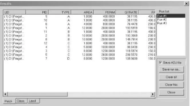
Output Files

Depending on which metrics are selected by the user, FRAGSTATS creates 4 output files corresponding to the three levels of metrics and the adjacency matrix. The user supplies a "basename" for the output files and FRAGSTATS appends the extensions .patch, .class, .land and .adj to the basename. All files created are comma-delimited ASCII files and viewable. These files are formatted to facilitate input into spreadsheets and database management programs:

• "basename".patch file.–Contains the patch metrics; the file contains 1 record (row) for each patch in the landscape; columns represent the selected patch metrics. If a batch file is analyzed, the file contains 1 record for each patch in each landscape specified in the batch file. The first record is a column header consisting of the acronyms for all the metrics that follow. For a single landscape, the patch output file would be structured as follows:

LID, PID, TYPE, AREA, PERIM, GYRATE, CORE D:\testgrid, 9, forest, 1.0000, 400.0000, 38.1195, 0.1600 D:\testgrid, 0, shrub, 4.0000, 800.0000, 76.4478, 1.9600

Etc.

• "basename".class file.–Contains the class metrics; the file contains 1 record (row) for each class in the landscape; columns represent the selected class metrics. If a batch file is analyzed, the file contains 1 record for each class in each landscape specified in the batch file. The first record is a column header consisting of the acronyms for all the metrics that follow. For a single landscape, the class output file would be structured as follows:

LID, TYPE, CA, PLAND, NP, PD, LPI D:\testgrid, forest, 8.0000, 22.5000, 4, 5.0000, 15.000 D:\testgrid, shrub, 21.0000, 26.2500, 3, 3.7500, 12.500

Etc.

• "basename".land file.–Contains the landscape metrics; the file contains 1 record (row) for the landscape; columns represent the selected landscape metrics. If a batch file is analyzed, the file contains 1 record for each landscape specified in the batch file. The first record is a column header consisting of the acronyms for all the metrics that follow. For a single landscape, the landscape output file would be structured as follows:

LID, TA, NP, PD, LPI, TE, ED D:\testgrid, 80.0000, 12, 15.0000, 15.0000, 7800.0000, 97.500

• “basename”.adj file.–Contains the class adjacency matrix; the file contains a simple header in addition to 1 record (row) for each class in the landscape, and is given in the form of a 2-way matrix. Specifically, first record contains the input file name, including the full path. The second record and first column contain the class IDs (i.e., the grid integer values associated with each class), and the elements of the matrix are the tallies of cell adjacencies for each pairwise combination of classes. For a single landscape, the adjacency output file would be structured as follows:

D:\testgrid

Class ID / ID, 2, 3, 4, 5, Background 2, 6840, 130, 120, 10, 0

(8)

3, 120, 7960, 160, 40, 10 4, 100, 140, 9880, 40, 20 5, 10, 40, 30, 3080, 16

Note, the adjacency tallies are generated from the double-count method in which each cell side is counted twice–at least for all positively-valued nonbackground cells–and only the 4 orthogonal neighbors are considered. In addition, the matrix may not be symmetrical if a landscape border is present because landscape boundary edges are only counted once. For example, a cell of class 3 (inside the landscape) adjacent to a cell of class -5 (in the landscape border) results in an adjacency for class 3; specifically, a 3 (row) -5 (column) adjacency. It does not result in an adjacency for class 5 (row), because the border cells themselves are not evaluated. For this reason, the adjacency matrix must be read as follows: each row represents the adjacency tallies for cells of that class, and the sum of adjacencies across all columns represents the total number of adjacencies for that class. These row totals should equal the number of positively-valued cells (i.e., inside the landscape) of the corresponding class times 4 (i.e., 4 surfaces for each cell). These row totals are used in several of the contagion metrics. Note that the adjacency matrix includes a column for background adjacencies, which represent cell surfaces of the corresponding class adjacent to designated background. If there is no specified background in the input landscape and a landscape border is not present, then the background adjacencies represent the cell surfaces along the landscape boundary–which are treated as background in the absence of a border. If a border is provides and no background is specified, then the background adjacencies with equal zero because every cell surface, including those along the landscape boundary, will be adjacent to a real non-background class. If a batch file is analyzed, the adjacency matrices corresponding to each landscape specified in the batch file are appended to the same file.

Backgrounds, Borders, and Boundaries

FRAGSTATS accepts images in several forms, depending on whether the image contains

background, and whether the landscape contains a border outside the landscape boundary (Fig. 1). The distinction among background, border, and boundary and how

they affect the landscape analysis and the calculations of various metrics is a source of great confusion. Care should be taken to fully understand these distinctions before trying to run FRAGSTATS. We strongly suggest that you read through this section twice, once to familiarize yourself with the terminology and a second time to understand the implications.

(9)

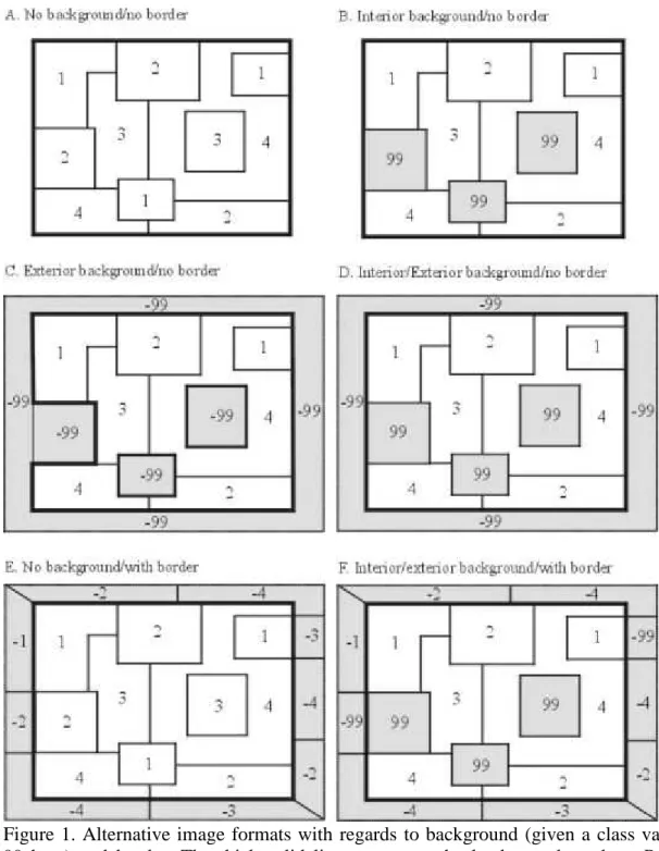
Figure 1. Alternative image formats with regards to background (given a class value of 99 here) and border. The thick solid line represents the landscape boundary. Positive values are ‘inside’ the landscape of interest and contribute to the computed total landscape area; negative values are ‘outside’ the landscape of interest and are only utilized to determine edge types for patches along the landscape boundary.

Every image will include a landscape boundary that defines the perimeter of the landscape and surrounds the patch mosaic of interest. The boundary is simply an invisible line around the patch mosaic of interest. It is not given explicitly in the image; rather, it is defined by an imaginary line around the outermost cells of positively valued cells. The

(10)

landscape boundary distinguishes between cells inside the landscape of interest from those outside, and thus ultimately determines the total landscape area. All positively valued cells are assumed to be inside the landscape of interest and are thus included in the total area of the landscape, regardless of whether they are classified as background (see below) or not. This is important, because many metrics include total landscape area in their calculation. Note, in most cases the landscape boundary will surround a single contiguous region of positively valued cells. However, it is possible to have disjunct regions of positively valued cells. In this case, the landscape boundary is not a single continuous line around the landscape of interest, but rather separate boundaries around each disjunct region of interest. The important point is that positively valued cells are

inside the landscape of interest, while negatively valued cells are outside, and the

landscape boundary is the imaginary line(s) that separate inside from outside. Hence, if the input image contains all positively valued cells, then the entire grid is assumed to be in the landscape of interest and the landscape boundary represents an imaginary line around the entire grid. If the input image contains negatively valued cells, then those cells are assumed to be outside the landscape of interest and thus outside the landscape boundary. In this case, the edge between positively and negatively valued cells represents the landscape boundary. The landscape boundary is important in the absence of a landscape border (see below) because FRAGSTATS needs to know how to treat the edges along the boundary in all edge calculations. In the absence of a border, the landscape boundary will be treated according to user specifications (see below).

An image may include background (also referred to as ‘mask’)--an undefined area either ‘interior’ or ‘exterior’ to the landscape of interest. Note that background can exist as ‘holes’ in the landscape and/or can partially or completely surround the landscape of interest. The background value can be any integer value. Positively valued cells of background are assumed to be ‘inside’ the landscape of interest; negatively valued cells of background are assumed to be ‘outside’ the landscape of interest. This distinction is important, as noted above, because positively valued background (interior background) will be included in the total landscape area, and thus affect many metrics, even though it will not be treated as a patch per se (see below). Further, via the graphical user interface (see below), any class or combination of classes can be treated (i.e., reclassified) as background for a particular analysis. There are several critical issues regarding how background is handled by FRAGSTATS:

1. Interior background (i.e., positively valued background) is included in the total landscape area and thus effects metrics that include total landscape area in their calculations. However, and this is quite tricky, interior background is in essence excluded from the total landscape area in a number of class and landscape metrics that involve summarizing patch or class metrics. For example, mean patch area is based on the average size of patches at the class or landscape level. If interior background is present, mean patch size as computed by FRAGSTATS will not equal the total landscape area divided by the number of patches, because the total landscape area includes background area not accounted for in any patch. Similarly, the area-weighted mean of any patch metric (i.e., distribution statistics at the class and landscape level; see FRAGSTATS Metrics documentation)

(11)

weights each patch by its proportional area representation. Here, the proportional area of each patch is not based on the total landscape area, but rather the sum of all patch areas, which is equivalent to the total landscape area minus interior background. Similarly, a number of landscape metrics are computed from the proportion of the landscape in each class (e.g., Shannon’s and Simpson’s diversity). Here, proportional area of each class is not based on total landscape area because the proportions must sum to 1 across all classes. Instead, the proportions are based on the sum of all class areas, which is equivalent to the total landscape area minus interior background. Given the subtle differences in how interior background affects various metrics, it behooves you to carefully read the FRAGSTATS Metrics documentation pertaining to each metric you choose, assuming of course that interior background is an issue.

2. Exterior background (i.e., negatively valued background) essentially has no effect on the analysis or on the computation of any metrics. Exterior background is assumed to be ‘outside’ the landscape of interest. Thus, the extent of exterior background in the input landscape has no effect.

3. Background (both interior and exterior) cells adjacent to non-background classes represent edges that must be accounted for in all edge-related metrics. The user specifies how background edge segments should be handled in all edge-related calculations (see below).

An image also may include a landscape border; a strip of land surrounding the landscape of interest (i.e., outside the landscape boundary) within which patches have been delineated and classified. Patches in the border must be set to the negative of the appropriate patch type code. For example, if a border patch is a patch type of code 34, then its cell value must be -34. The border can be any width (as long as it is at least 1 cell wide) and provides information on patch type adjacency for patches on the edge of the landscape (i.e., along the landscape boundary). Essentially, patches in the border provide information on patch type adjacency for patches in the landscape of interest located along the landscape boundary; all other attributes of the patches in the border are ignored because they are outside the landscape of interest. Thus, the border affects only metrics where patch type adjacency is considered: core area, edge contrast, contagion and interspersion metrics.

Under most circumstances, it is probably not valid to assume that all edges function the same. Indeed, there is good evidence that edges vary in their affects on ecological processes and organisms depending on the nature of the edge (e.g., type of adjacent patches, degree of structural contrast, orientation, etc.). Accordingly, the user can specify a file containing edge contrast weights (described in more detail in the Contrast Metrics section of the FRAGSTATS Metrics documentation) for each combination of patch types (classes), including adjacencies involving background if it exists. Briefly, these weights represent the magnitude of edge contrast between adjacent patch types and must range between 0 (no contrast) and 1 (maximum contrast). Edge contrast weights are used to compute several edge-based metrics. If this weight file is not provided, these edge

(12)

contrast metrics are simply not computed. Generally, if a landscape border is designated, a weight file will be specified as well, because one of the principal reasons for specifying a border is when information on edge contrast is deemed important. If a border is present, the edge contrast associated with all landscape boundary edge segments is made explicit due to knowledge of the abutting patch types. If a border is absent, then all edge segments along the landscape boundary are treated the same as background, as specified in the user-provided edge contrast weight file. Note, however, that the presence of a landscape border will have no affect on the edge contrast metrics if a contrast weight file is not specified--because these metrics will not be computed.

Similarly, the user can specify a file containing edge depths (described in more detail in the Core Area Metrics section of the FRAGSTATS Metrics documentation) for each combination of patch types (classes), including adjacencies involving background if it exists. Briefly, edge depths represent the distance at which edge effects penetrate into a patch and must be given in distance units (meters); edge depths can be any number ≥ 0. However, when implementing edge depths for the purpose of determining core areas, FRAGSTATS is constrained by minimum resolution established by the cell size. Thus, in effect, edge depths will be rounded to the nearest distance in increments of the cell size. For example, if the cell size is 30 m, and you specify a 100 m edge depth, the edge mask used to mask cells along the edge of a patch (i.e., eliminate them from the “core” of the patch) will be 3 cells wide (90 m), because it is not possible to use a mask that is 3.3 cells wide. Similarly, a specified edge depth of 50 m will in effect be rounded up to 2 cells (60 m). Therefore, it is generally advisable to specify edge depths in increments equal to the cell size. Edge depths are used to compute several core area-based metrics. If this edge depth file is not provided, these core area metrics are simply not computed. Typically, if a landscape border is designated, an edge depth file will be specified as well, because one of the principal reasons for specifying a border is when information on edge effects is deemed important. If a border is present, the edge depths associated with all landscape boundary edge segments is made explicit due to knowledge of the abutting patch types. If a border is absent, then all edge segments along the landscape boundary are treated the same as background, as specified in the user-provided edge depth file. Note, however, that the presence of a landscape border will have no affect on the core area metrics if an edge depth file is not specified–because these metrics will not be computed.

A landscape border is also useful for determining patch type adjacency for the contagion and interspersion indices. These metrics (described in more detail in the Contagion and Interspersion Metrics section of the FRAGSTATS Metrics documentation) require information on cell adjacency; that is, the abutting class values for the side of every cell. The proportional distribution of cell adjacencies is used to compute a variety of landscape texture metrics. Although a landscape border is not often designated for the primary purpose of computing these texture metrics, a border will inform the calculation of these metrics. If a border is present, the adjacencies associated with all landscape boundary edge segments is made explicit due to knowledge of the abutting patch types. If a border is absent, then all edge segments along the landscape boundary are treated the same as background and the corresponding cell adjacencies are ignored in the calculation of these metrics.

(13)

Metrics based on edge length (e.g., total edge or edge density) are affected by these considerations as well. If a landscape border is present, then edge segments along the boundary are evaluated to determine which segments represent ‘true’ edge and which do not. For example, an edge segment between cells with class value 5 (inside the landscape of interest) and cells with class value -5 (outside the landscape of interest; i.e., in the border) does not represent a true edge; in this case, the landscape boundary artificially bisects an otherwise contiguous patch and the edge is not counted in the calculations of total edge length. Conversely, an edge segment between class 5 and -3 represents a true

edge and is counted. If a landscape border is absent, then a user-specified proportion of

the landscape boundary is treated as true edge and the remainder is ignored. For example, if the user specifies that 50% of the landscape boundary should be treated as true edge, then 50% of the landscape boundary will be incorporated into the edge length metrics. Regardless of whether a landscape border is present or not, if a background class is specified, then a user-specified proportion of edge bordering background is treated as

true edge and the remainder is ignored.

We recommend including a landscape border, especially if edge contrast, core area, or patch type adjacency is deemed important. In most cases, some portions of the landscape boundary will constitute ‘true’ edge (i.e., an edge with a contrast weight > 0) and others will not, and it will be difficult to estimate the proportion of the landscape boundary representing true edge. Moreover, it will be difficult to estimate the average edge contrast weight or edge depth for the entire landscape boundary. Thus, the decision on how to treat the landscape boundary will be somewhat subjective and may not accurately represent the landscape. In the absence of a landscape border, the affects of the decision regarding how to treat the landscape boundary on the landscape metrics will depend on landscape extent and heterogeneity. Larger and more heterogeneous landscapes will have a greater internal edge-to-boundary ratio and therefore the boundary will have less influence on the landscape metrics. Of course, only those metrics based on edge lengths and types are affected by the presence of a landscape border and the decision on how to treat the landscape boundary. When edge-based metrics are of particular importance to the investigation and the landscapes are small in extent and relatively homogeneous, the inclusion of a landscape border and the decision regarding the landscape boundary should be considered carefully.

So, let’s try to put all of this together. There are five types of metrics affected by landscape boundary, background, and border designations: (1) total landscape area, (2) edge length metrics, (3) core area metrics, (4) contrast metrics, and (5) contagion/interspersion metrics. Let’s consider several scenarios involving various combinations of background and border, and how each of these types of metrics will be treated under each scenario.

• Scenario 1.–Input landscape contains all positively valued cells of non-background classes (Fig. 1a). In this case, the entire grid is assumed to be in the landscape of interest and every cell belongs to a non-background class. The landscape boundary surrounds the entire grid and there is no border or background present.

(14)

Total landscape area.–All cells are included in the total landscape area

calculation.

Edge length metrics.–User must specify the proportion of the landscape boundary

to include as edge. All other edges are explicit.

Core area metrics.–The landscape boundary is treated like background; the user

must specify the edge depth for cells abutting background in the edge depth file, and this depth is applied to the landscape boundary. All other edges are explicit; their edge depths are specified in the edge depth file.

Contrast metrics.–The landscape boundary is treated like background; the user

must specify the edge contrast for cells abutting background in the edge contrast weight file, and this weight is applied to the landscape boundary. All other edges are explicit; their edge contrast weights are specified in the edge contrast weight file.

Contagion/interspersion metrics.–The landscape boundary is treated like

background and is simply ignored since there is no information available on patch type adjacency.

• Scenario 2.–Input landscape contains all positively valued cells, but includes a background class (Fig. 1b). In this case, the entire grid is assumed to be in the landscape of interest , but some cells belong to a background class. Here, the background is interior because it is positively valued and thus inside the landscape of interest. The landscape boundary surrounds the entire grid and there is no border present.

Total landscape area.–All cells are included in the total landscape area

calculation.

and background edges to include as edge. All other edges are explicit.

Core area metrics.–The landscape boundary is treated like background; the user

must specify the edge depth for cells abutting background in the edge depth file, and this depth is applied to both the landscape boundary and background edges. All other edges are explicit; their edge depths are specified in the edge depth file.

Contrast metrics.–The landscape boundary is treated like background; the user

must specify the edge contrast for cells abutting background in the edge contrast weight file, and this weight is applied to both the landscape boundary and background edges. All other edges are explicit; their edge contrast weights are specified in the edge contrast weight file.

(15)

Contagion/interspersion metrics.–The landscape boundary and background are

treated similarly; both are simply ignored when evaluating adjacencies since there is no information available on patch type adjacency in either case.

• Scenario 3.–Input landscape contains a mixture of positively valued cells and negatively valued background cells (Fig. 1c). Note, it doesn’t matter whether the negatively valued background cells are located entirely on the periphery of the positively valued cells (i.e., outside the landscape of interest) or located as holes in the interior of the landscape, or a combination of the two. In all cases, the positively valued cells are is assumed to be inside the landscape of interest , whereas the negatively valued background cells are assumed to be outside the landscape of interest and thus outside the landscape boundary. Here, the background is entirely

exterior because it is all negatively valued and thus outside the landscape of interest.

The landscape boundary separates contiguous regions of positively valued cells from the negatively valued cells and there is no border present. Alternatively, the exterior background could be considered border, but the use of border is generally reserved for situations involving negatively valued non-background cells.

Total landscape area.–All positively valued cells are included in the total

landscape area calculation; negatively valued cells (here, all background) are ignored.

and background edges (in this case, they are the same) to include as edge. All other edges are explicit.

Core area metrics.–The landscape boundary is treated like background; in this

case, the entire landscape boundary is in fact also background. The user must specify the edge depth for cells abutting background in the edge depth file, and this depth is applied to the background edges (in this case, all on the landscape boundary). All other edges are explicit; their edge depths are specified in the edge depth file.

Contrast metrics.–The landscape boundary is treated like background; in this

case, the entire landscape boundary is in fact also background. The user must specify the edge contrast for cells abutting background in the edge contrast weight file, and this weight is applied to the background edges (in this case, all on the landscape boundary). All other edges are explicit; their edge contrast weights are specified in the edge contrast weight file.

Contagion/interspersion metrics.–The landscape boundary and background (in

this case, they are the same) are treated similarly; they are simply ignored when evaluating adjacencies since there is no information available on patch type adjacency.

(16)

• Scenario 4.–Input landscape contains a mixture of positively valued cells, including some positively valued background cells, and negatively valued background cells (Fig. 1d). Note, as in scenario 3, it doesn’t matter whether the negatively valued background cells are located entirely on the periphery of the positively valued cells (i.e., outside the landscape of interest) or located as holes in the interior of the landscape, or a combination of the two. In all cases, the positively valued cells are is assumed to be inside the landscape of interest , whereas the negatively valued background cells are assumed to be outside the landscape of interest and thus outside the landscape boundary. Here, the background is a combination of interior and

exterior background. The landscape boundary separates contiguous regions of

positively valued cells from the negatively valued cells and there is no border present. As noted in scenario 3, the exterior background could be considered border, but the use of border is generally reserved for situations involving negatively valued non-background cells.

Total landscape area.–All positively valued cells, including the ‘interior’

background, are included in the total landscape area calculation; negatively valued cells (here, all background) are ignored.

(in this case, all background) and interior background edges to include as edge. All other edges are explicit.

Core area metrics.–The landscape boundary is treated like background; in this

case, the entire landscape boundary is in fact also background. The user must specify the edge depth for cells abutting background in the edge depth file, and this depth is applied to all background edges (in this case, both on the landscape boundary and interior). All other edges are explicit; their edge depths are specified in the edge depth file.

Contrast metrics.–The landscape boundary is treated like background; in this

case, the entire landscape boundary is in fact also background. The user must specify the edge contrast for cells abutting background in the edge contrast weight file, and this weight is applied to all background edges (in this case, both on the landscape boundary and interior). All other edges are explicit; their edge contrast weights are specified in the edge contrast weight file.

Contagion/interspersion metrics.–The landscape boundary (in this case, all

background) and interior background are treated similarly; both are simply ignored when evaluating adjacencies since there is no information available on patch type adjacency in either case.

• Scenario 5.–Input landscape contains a mixture of positively valued non-background cells and negatively valued non-background cells (i.e., a true border; Fig. 1e). In this case, the positively valued cells are is assumed to be inside the landscape of interest , whereas the negatively valued cells are assumed to be outside the landscape of

(17)

interest and thus outside the landscape boundary. The landscape boundary separates contiguous regions of positively valued cells from the negatively valued cells; no background exists; and there is a true border present. This is perhaps the ideal

scenario because every cell is classified into a real class (i.e., no background) and a

border is included to inform all edge, core, and adjacency calculations.

Total landscape area.–All positively valued cells are included in the total

landscape area calculation; negatively valued cells are ignored.

Edge length metrics.–Because a border is present and there is no background, all

edges are explicit; that is, the image provides explicit information on whether every edge segment along the boundary is a true edge or not. In this case, the user does not need to specify the proportion of the landscape boundary to include as edge. In fact, any user specification in this regard via the user interface will be disregarded.

Core area metrics.–Because a border is present and there is no background, all

edges are explicit; that is, the image provides explicit information on the abutting patch types along the boundary. In this case, all edge depths are specified in the edge depth file.

Contrast metrics.–Because a border is present and there is no background, all

edges are explicit; that is, the image provides explicit information on the abutting patch types along the boundary. In this case, all edge contrast weights are specified in the edge contrast weight file.

Contagion/interspersion metrics.–Because a border is present and there is no

background, all edges are explicit; that is, the image provides explicit information on the abutting patch types along the boundary. In this case, all boundary edge segments are included in the adjacency calculations.

• Scenario 6.–Input landscape contains a mixture of positively valued cells, including both background and non-background classes, and negatively valued cells, including both background and non-background classes (Fig. 1f). This is the most complex scenario involving a complicated mixture in interior and exterior background and a border. In this case, all positively valued cells (including interior background) are is assumed to be inside the landscape of interest, whereas the negatively valued cells are assumed to be outside the landscape of interest and thus outside the landscape boundary. The landscape boundary separates contiguous regions of positively valued cells from the negatively valued cells. A true border is present, but it includes some background class. This is perhaps also an ideal scenario, like scenario 5, but contains a realistic, sometimes unavoidable, situation in which some areas must be classified as background, either because there is no information available from which to classify them, or because it is deemed desirable ecologically to treat these areas as undefined background.

(18)

Total landscape area.–All positively valued cells, including the interior

background, are included in the total landscape area calculation; negatively valued cells are ignored.

Edge length metrics.–Because a border is present but contains some background

and there is interior background, only a portion of edges are explicit; that is, some edges abut background (either interior or exterior) and it is not explicit whether they represent true edge or not. In this case, the user must specify the proportion of edges involving background to include as edge.

Core area metrics.–Because a border is present but contains some background

and there is interior background, only a portion of edges are explicit. Here, all boundary edges involving background and interior background edges are treated the same. The user must specify the edge depth for cells abutting background in the edge depth file, and this depth is applied to all background edges (in this case, both on the landscape boundary and interior). All other edges are explicit; their edge depths are specified in the edge depth file.

Contrast metrics.–Because a border is present but contains background, and there

is interior background, only a portion of edges are explicit. Here, all boundary edges involving background and interior background edges are treated the same. The user must specify the edge contrast weight for cells abutting background in the edge contrast weight file, and this weight is applied to all background edges (both on the landscape boundary and interior). All other edges are explicit; their contrast weights are specified in the edge contrast weight file.

Contagion/interspersion metrics.–Because a border is present but contains some

background, and there is interior background, only a portion of edges are explicit. In this case, edge segments involving background (both on the landscape boundary and interior) are ignored in the adjacency calculations.

Installation

FRAGSTATS installation is quick and easy (hopefully). After downloading the fragstats.zip file, simply double click on the file and Winzip should open (if you don’t have Winzip or another file compression utility that can unzip files, you will need to download Winzip from the web). In Winzip, simply click on the “install” button and follow the onscreen instructions. Alternatively, you can extract the zipped files to a folder and click on the setup.exe file and follow the instructions; however, this approach will not automatically delete the installation files after the installation is complete. Once installed, FRAGSTATS is run by double clicking your mouse on the Fragstats.exe file. However, if you are using FRAGSTATS with Arc Grids, then ArcView Spatial Analyst or ArcGIS must be installed on your computer and FRAGSTATS must have access to the dll libraries found in the ArcView Bin32 or ArcGIS Bin directory. Specifically, the Fragstats.exe file must either be located and run from the same directory as the dll libraries (not the best option) or a path to the dll libraries must be specified in your environmental variables (preferable) or in the autoexec.bat file. For detailed instructions

(19)

on installing Fragstats for use with ArcGrids, see the discussion on Overview--Data Formats.

Data Formats

FRAGSTATS accepts raster images in a variety of formats, including ArcGrid, ASCII, BINARY, ERDAS, and IDRISI image files. FRAGSTATS does not accept Arc/Info vector coverages like the earlier version 2. All input data formats have the following common requirements:

• All input grids should be signed integer grids containing all non-zero class values (i.e., each cell should be assigned an integer value corresponding to its class membership or patch type). Note, FRAGSTATS assumes that the grids are ‘signed’ integer grids; inputting an ‘unsigned’ integer grid may cause problems. In addition, note that assigning the zero value to a class is allowable, but can cause problems in the moving window analysis if it is not specified as the background class. Specifically, if zero is specified as the background class, FRAGSTATS will reclassify all zero cell values to a new class value equal to 1 plus the largest class value in the input landscape. This procedure is necessary because a zero background class value will cause problems in the moving window analysis because a background value of zero in the output grid cannot be distinguished from a computed metric value of zero. In addition, a zero class value will cause problems when the landscape contains a border because zero cannot be negative, yet all cells in the border must be negative integers). Thus, all zero cells are assumed to be interior (i.e., inside the landscape of interest). If a moving window analysis is selected and the input grid contains zeros and zero is NOT specified as the background class, then execution will be stopped and an error message reported to the log file. For these reasons, it is best to avoid the use of zero class values altogether.

• All input grids should consist of square cells with cell size specified in meters. For certain input formats (ASCII and BINARY), this is not an issue because cells are assumed to be square and you are required to enter the cell size (in meters) in the graphical user interface. However, FRAGSTATS assumes that all other image formats (ArcGrid, ERDAS, and IDRISI) include header information that defines cell size. Consequently these images must have a metric projection (e.g., UTM) to ensure that cell size is given in metric units.

There are some additional special considerations for each input data format, as follows: (1) Arc Grid created with Arc/Info. Note, to use Arc Grids you must have ArcView Spatial Analyst or ArcGIS installed on your computer and FRAGSTATS must have access to a certain .dll file found either in the ArcView Bin32 directory (for ArcView Spatial Analyst users) or the ArcGIS Bin directory (for ArcGIS users). Specifically, a path to the corresponding dll library file should be specified in the environmental settings under NT or Windows 2000 operating systems, or a path statement included in the autoexec.bat file, e.g., under Windows 98, as follows:

(20)

Windows NT: You can add the necessary Path variable or edit the existing one via the Control panel - System Properties - Environment tab. Add a new variable or edit the existing Path variable in the system variables, not the user variables (this will require administrative privileges). Add the full path to the appropriate .dll file. If you are using ArcView Spatial Analyst, the required file is the avgridio.dll file and it is typically installed in the following path: \esri\av_gis30\arcview\bin32. If you are using ArcGIS, the required file is the aigridio.dll file and it is typically installed in the following path: \esri\arcinfo\arcexe81\bin. Note, your software version number and path may be different so be sure to locate the .dll file on your computer and enter the correct path. If you are using both Spatial Analyst and ArcGIS, then you can enter either or both paths to the Path system variable.

Windows 2000/XP: You can add the necessary Path variable or edit the existing one via the Control panel - System Properties - Advanced tab - Environment Variables button. Add a new variable or edit the existing Path variable in the system variables, not the user variables (this will require administrative privileges). Then, following the instructions above for Windows NT.

Windows 95/98: You must add the necessary Path statement to the autoexec.bat file. First, search your computer for the autoexec.bat file and open it using any text editor. Then, either add a Path statement or edit the existing one. Add the full path to the appropriate .dll file. If you are using ArcView Spatial Analyst, the required file is the avgridio.dll file and it is typically installed in the following path: \esri\av_gis30\arcview\bin32. If you are using ArcGIS, the required file is the aigridio.dll file and it is typically installed in the following path: \esri\arcinfo\arcexe81\bin. Thus, the path statement should look something like: PATH c:\esri\av_gis30\arcview\bin32. Note, your software version number and path may be different so be sure to locate the .dll file on your computer and enter the correct path. If you are using both Spatial Analyst and ArcGIS, then you can enter either or both paths to the Path system variable. If you are adding the path to an existing path, simple use a semicolon to separate the unique paths in the Path statement. After saving the file you will need to reboot your machine for the change to take effect.

(2) ASCII file, no header. Each record should contain 1 image row. Cell values should be separated by a comma or a space(s). Note, it will be necessary to strip (delete) the header information from the image file if it exists, but be sure to keep it for later reference regarding background cell value, # rows, and # columns.

(3) 32-bit binary file, no header; no other limitations.

(21)

(5) ERDAS image files (.gis, .lan, and .img). FRAGSTATS accepts images from both ERDAS 7 (.gis and .lan) and ERDAS 8 (.gis, .lan, and .img), but the limitations are somewhat different, as follows:

ERDAS 8 Files.–FRAGSTATS accepts .gis, .lan, and .img files used by current versions of ERDAS IMAGINE, including signed 8-, 16-, and 32-bit integer grids. While .gis and .lan file formats are supported, their limitations make them less practical than .img (see discussion of ERDAS 7 files below). Care should be taken when preparing the data to be used with FRAGSTATS, especially when importing data from other formats (for instance from Arc Grid). Be sure to set the import options to ‘signed integer’. Regardless of the input integer format (8-, 16-, or 32-bit), the patch ID output file created by FRAGSTATS will be a signed 32-bit integer, and if moving window analysis is selected, all output grids will be 32-bit floating point. Multi-layered files are not rejected, but only layer one is processed and the outputs are all single layered. As noted above, cells must be square, not rectangular, and the measurement unit should be meters. If the measurement unit is not specified, then it is assumed to be meters. The cell size and measurement unit specification can be changed within ERDAS Imagine using the ImageInfo tool -> Change Map Model from the Edit menu. The projection information existing in the input file is passed unchanged to the output files. FRAGSTATS does not use this information internally.

ERDAS 7 files.-- FRAGSTATS accepts .gis and .lan files used by ERDAS 7, which are limited to unsigned 8- or 16-bit integer grids. FRAGSTATS will accept both 8-bit and 16-bit integer files and it will reject multi-layered files. While .gis and .lan file formats are supported, their limitations make them less practical than .img. In particular, ERDAS 7.x files are limited to unsigned integers (i.e., only positive integers), therefore landscape borders (which require negative class values) cannot be represented. Another consequence of this particular limitation is that FRAGSTATS-generated patch ID files will not fill the non-landscape cells (i.e., no data cells) with the usual value (minus the background class value), but with zero values. The restriction to 8- or 16-bit integers imposes some limitations when using the FRAGSTATS on large grids. Specifically, unsigned 16-bit integers can only take on values up to 65,534. Thus, class ID values are limited to integers within this range (note, this should not be a problem, since it is unlikely that anyone would have more than 65,534 patch types). Similarly, patch ID values in the patch ID output grid optionally produced by FRAGSTATS are limited to the same range, effectively limiting the number of patches in this output grid to 65,534. If the grid contains more than this number of patches, FRAGSTATS will not be able to output a unique ID for each patch and the user will have to somehow distinguish among patches with the same ID. Finally, because the moving window analysis requires 32-bit output files (in

(22)

order to output floating point values), moving window analysis is not supported with ERDAS 7 files.

(6) IDRISI image files (.rdc). IDRISI currently supports signed 8- or 16-bit integers and

32-bit floating point grids. This imposes some limitations when using the FRAGSTATS

on large grids. Specifically, signed 16bit integers can only take on values between -32,768 and 32,767. Thus, class ID values are limited to integers within this range (note, this should not be a problem, since it is unlikely that anyone would have more than 32,767 patch types). Similarly, patch ID values in the patch ID output grid optionally produced by FRAGSTATS are limited to the same range, effectively limiting the number of patches in this output grid to 37,767. If the grid contains more than this number of patches, FRAGSTATS will not be able to output a unique ID for each patch and the user will have to somehow distinguish among patches with the same ID. Fortunately, IDRISI supports 32-bit floating point grids, which are produced in a moving window analysis.

Step 1. Starting the FRAGSTATS GUI

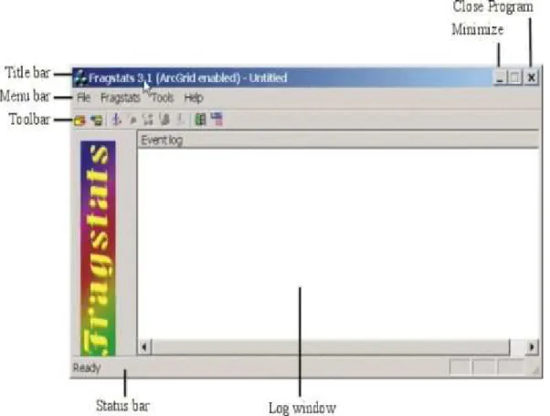
To start FRAGSTATS, simply double click on the Fragstats.exe file and (hopefully) the opening FRAGSTATS window will display (Fig. 2).

Figure 2. Anatomy of the FRAGSTATS opening user interface.

The anatomy of this opening window is quite simple, as it is similar to most windows-based programs. The title bar lists the name of the current or open parameterization file. The parameterization file contains the current parameterization scheme. When you first

(23)

start FRAGSTATS, a parameterization file does not exist. Consequently, the title is listed as “untitled” until you save the current parameterization scheme under the File-Save option. Once you have saved the current parameterization or have retrieved a previously saved scheme, the title bar will list the open parameterization file. The menu bar consists of a few items that allow you to parameterize a FRAGSTATS run, edit certain files, and save and retrieve parameterization files. Each menu item has a drop-down list of options. The toolbar provides quick access to the frequently used File and Fragstats menu options. The log window provides a running log of the analysis. The status bar indicates the status of the program. Details of the parameterization process are described in Step 2. Here, each of the menu bar items are briefly described:

File Menu.–The File menu allows you to open an existing parameterization file or save

the current parameterization file. Note, parameterization files are given the file extension .frg.

1. New.–Creates a new (or blank) parameterization file. It is not necessary to begin by creating a new file. A new file is automatically opened when you start FRAGSTATS. This option is used when you have a parameterization file currently open and wish to create a new file from scratch.

2. Open.–Opens an existing (previously saved) parameterization file.

3. Save.–Saves the current parameterization to a file with the extension .frg. Note, if you are saving a parameterization file for the first time, you will be prompted to specify a location and file name. If you are saving from an open parameterization file, this will overwrite the existing file without prompting you for a file name. This file contains all the parameter settings in the dialog boxes at the time the file was saved. This can be very useful if you are running FRAGSTATS repeatedly with the same or similar parameterization schemes.

4. Save as.–Saves the current parameterization file to a location and file name that you specify.

5. Exit.–Closes the program. The same effect is achieved by clicking on the X in the upper right corner of the window.

Fragstats Menu.–The Fragstats menu allows you to parameterize the analysis.

1. Set Run Parameters.–Opens a new dialog box that allows you to specify necessary parameters for running FRAGSTATS (see Step 2).

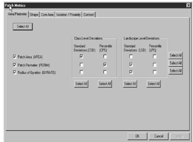
2. Select Patch Metrics.–Opens a new dialog box that allows you to select and parameterize the desired patch-level metrics. Note, this function is not active until the

Run Parameters dialog box is successfully completed, and then only if patch metrics

are selected in the run parameters.

(24)

3. Select Class Metrics.–Opens a new dialog box that allows you to select and parameterize the desired class-level metrics. Note, this function is not active until the

Run Parameters dialog box is successfully completed, and then only if class metrics

are selected in the run parameters.

4. Select Landscape Metrics.–Opens a new dialog box that allows you to select and parameterize the desired landscape-level metrics. Note, this function is not active until the Run Parameters dialog box is successfully completed, and then only if

landscape metrics are selected in the run parameters.

5. Clear All Menus.–Clears the Run Parameters, Patch-, Class-, and Landscape Metrics dialog boxes.

6. Execute Fragstats.–Executes a FRAGSTATS run. An “execution finished” message will appear in the log window when FRAGSTATS processing is complete.

Tools Menu.–The Tools menu provides you with several miscellaneous options for

creating and editing batch files, reclassifying classes and controlling class-level output, browsing results, and saving the log file.

1. Batch File Editor.–Allows you to create and edit batch files. See Step 4 on Using Batch Files for details on the batch file editor.

2. Class Properties.–Allows you to edit the properties of each class; that is, designate classes as background and disable the output for selected classes. See Step 5 on Modifying Class Properties for details.

3. Browse Results.–Allows you to browse and save the results of the analysis. See Step 7 on Browsing and Saving Results for details.

4. Clear Log.–Clears the log window of all text.

5. Save Log.–Saves the log window as an ASCII text file with the extension .log to a location and file name that you specify.

Help Menu.–The Help menu provides you with online help.

1. Help Content.–Allows you to access a familiar windows-based help interface with the standard content, index, and find options. The online help information is essentially the same as provided in this document and the FRAGSTATS Metrics document.

(25)

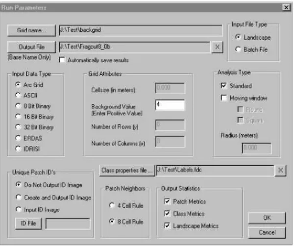
Step 2. Setting Run Parameters

After opening the FRAGSTATS interface, the