Adaptively Lossy Image Compression for Onboard Processing

Title Page

Adaptively Lossy Image Compression for Onboard Processing

by

Justin Goodwill

B.S. Electrical Engineering, University of Pittsburgh, 2018

Submitted to the Graduate Faculty of the Swanson School of Engineering in partial fulfillment

of the requirements for the degree of

Master of Science in Electrical and Computer Engineering

University of Pittsburgh 2020

Committee Page

UNIVERSITY OF PITTSBURGH SWANSON SCHOOL OF ENGINEERING

This thesis was presented by

Justin Goodwill

It was defended on March 6, 2020 and approved by

Dr. Zhi-Hong Mao, Ph.D., Professor, Department of Electrical and Computer Engineering, Department of Bioengineering

Dr. Ahmed Dallal, Ph.D., Assistant Professor, Department of Electrical and Computer Engineering

Thesis Advisor: Dr. Alan George, Ph.D., Department Chair and Mickle Chair Professor, Department of Electrical and Computer Engineering

Copyright © by Justin Goodwill 2020

Abs tract

Adaptively Lossy Image Compression for Onboard Processing

Justin Goodwill, MS University of Pittsburgh, 2020

More efficient image-compression codecs are an emerging requirement for spacecraft because increasingly complex, onboard image sensors can rapidly saturate downlink bandwidth of communication transceivers. While these codecs reduce transmitted data volume, many are compute-intensive and require rapid processing to sustain sensor data rates. Emerging next-generation small satellite (SmallSat) computers provide compelling computational capability to enable more onboard processing and compression than previously considered. For this research, we apply two compression algorithms for deployment on modern flight hardware: (1) end-to-end, neural-network-based, image compression (CNN-JPEG); and (2) adaptive image compression through feature-point detection (FPD-JPEG). These algorithms rely on intelligent data-processing pipelines that adapt to sensor data to compress it more effectively, ensuring efficient use of limited downlink bandwidths. The first algorithm, CNN-JPEG, employs a hybrid approach adapted from literature combining convolutional neural networks (CNNs) and JPEG; however, we modify and tune the training scheme for satellite imagery to account for observed training instabilities. This hybrid CNN-JPEG approach shows 23.5% better average peak signal-to-noise ratio (PSNR) and 33.5% better average structural similarity index (SSIM) versus standard JPEG on a dataset collected on the Space Test Program – Houston 5 (STP-H5-CSP) mission onboard the International Space Station (ISS). For our second algorithm, we developed a novel adaptive image-compression pipeline based upon JPEG that leverages the Oriented FAST and Rotated BRIEF (ORB) feature-point detection algorithm to adaptively tune the compression ratio to allow for a tradeoff between

PSNR/SSIM and combined file size over a batch of STP-H5-CSP images. We achieve a less than 1% drop in average PSNR and SSIM while reducing the combined file size by 29.6% compared to JPEG using a static quality factor (QF) of 90.

Table of Contents

Preface ... ix

1.0 Introduction ...1

2.0 Background ...6

2.1 Compression with Neural Networks ...7

2.1.1 TensorFlow Lite ... 10

2.1.2 Hardware Acceleration with FPGAs ... 10

2.2 Adaptive Compression ... 11

3.0 Approach ... 13

3.1 Compression with CNN-JPEG ... 14

3.2 Compression with FPD-JPEG ... 21

4.0 Results ... 23 4.1 CNN-JPEG Compression ... 23 4.2 FPD-JPEG Compression ... 36 5.0 Conclusions ... 45 6.0 Future Work ... 46 Bibliography ... 48

List of Tables

Table 1: Approximate Number of Parameters in Encoder Network for Color Images ...9 Table 2: Resource Utilization... 32

List of Figures

Figure 1: Observed Instabilities in Output Reconstruction ... 15

Figure 2: Observed Instabilities in Compact Representation ... 15

Figure 3: Reconstructed Images Exemplifying Poor Generalization to Test Set ... 18

Figure 4: SDSoC-Generated Streaming Architecture [33] ... 20

Figure 5: 2×2 Grid of Convolution Units [33] ... 21

Figure 6: PSNR vs. Bitrate... 23

Figure 7: SSIM vs. Bitrate ... 24

Figure 8: Distribution of Compression Ratios for Standard JPEG and CNN-JPEG ... 25

Figure 9: Visual Comparison of CNN-JPEG against Standard JPEG at Same Bitrate ... 27

Figure 10: Execution Time on Zynq-7020 ... 30

Figure 11: Execution Time on Zynq-MPSoC ... 31

Figure 12: Dynamic Power on Zynq-7020 ... 34

Figure 13: Dynamic Power on Zynq-MPSoC... 35

Figure 14: FPD-JPEG Compression SSIM Comparison ... 37

Figure 15: FPD-JPEG Compression PSNR Comparison ... 38

Figure 16: Comparison of Coastline at Different PSNR and SSIM ... 40

Figure 17: FPD-JPEG Execution Time on Zynq-7020 ... 42

Preface

This research was supported by SHREC industry and agency members and by the IUCRC Program of the National Science Foundation under Grant No. CNS-1738783.

The author would like to thank Dr. David Wilson (NASA GSFC), Dr. Christopher Wilson (NASA GSFC), and Sebastian Sabogal (University of Pittsburgh) for their collaborative efforts and insightful review of this work. The author would also like to extend thanks to Nicholas Franconi (NASA GSFC) for his exceptional mentorship as well as Dr. Alan George (University of Pittsburgh), David Langerman (University of Pittsburgh), Gary Crum (NASA GSFC), James MacKinnon (NASA GSFC), and Alessandro Geist (NASA GSFC) for their continued support and guidance on this research.

Finally, the author owes a debt of gratitude to his parents for their unwavering love, guidance, and support.

1.0 Introduction

When developing mission concepts and systems for satellites, mission designers must address design considerations balancing concessions between data storage, data processing, and communication bandwidth for their instruments. The spacecraft platform (i.e. from nanosatellite to large satellite) has requirements for size, weight, power, and cost (SWaP-C) that define general constraints in the trade-space for those considerations. The designer must then identify the best combination and balance of these traits for the mission. For example, more efficient image-compression codecs are an emerging requirement for spacecraft because increasingly complex, onboard sensors can rapidly saturate both downlink bandwidth of communication transceivers and onboard data storage capability. While these codecs can significantly reduce transmitted or stored data volume, many are computationally intensive and require rapid processing to sustain sensor data rates.

Traditional large spacecraft often rely upon slow, radiation-hardened (rad-hard) processing technologies due to the harsh space environment [1]-[2]. However, with the advent of more capable onboard processing systems, including hybrid rad-hard/commercial architectures or commercial-off-the-shelf (COTS) devices [3], developers are emphasizing more onboard processing and compression to address mission challenges. These hybrid and commercial systems provide substantial benefits in processing capability and power efficiency over their rad-hard counterparts, and benefit from significant advancements in hardware and software dependability, enabling their inclusion in a variety of mission classes and orbits. These systems can provide a several orders of magnitude increase in computational capacity, enabling more complex onboard sensor processing including intelligent image-compression techniques for both science and defense applications.

In recent years, multiple prominent examples of these space computer architectures featuring hybrid system-on-chips (SoCs) have been developed for 1U and 3U spacecraft [4]-[5]. Developed by the National Science Foundation (NSF) Center for Space, High-performance, and Resilient Computing (SHREC), the CHREC Space Processor (CSP) [4] and its successor, the SHREC Space Processor (SSP), include the Xilinx Zynq-7000 APSoC (Zynq-7020 for CSP and selectable Zynq-7030 or Zynq-7045 for SSP), which is comprised of a dual-core ARM Cortex-A9 processor and a 28-nm Artix-7 (CSP) or 28-nm Kintex-7 (SSP) FPGA fabric. Developed by NASA Goddard Space Flight Center (GSFC), the SpaceCube v3.0 [5] includes a Xilinx Zynq UltraScale+ MPSoC (Zynq-MPSoC, ZU7EV), which incorporates a quad-core ARM Cortex-A53 and a 16-nm UltraScale Architecture FPGA fabric. There are additional single-board processors using these same devices listed in [3].

The development of more capable methods for data reduction and data triage is a critical concern for NASA highlighted in the 2015 NASA Technology Roadmaps [2] under TA 11: Modeling, Simulation, Information Technology, and Processing, specifically, 11.1.1 Flight Computing and 11.4.1.4 Onboard Data Capture and Triage Methodologies. This demand was also acknowledged by the National Research Council of the National Academies in the assessment of the technology roadmap in [6] and [7]. 11.4.1.4 specifically describes, “Apply novel machine learning capabilities onboard to support data reduction.” In this technology description, NASA defines a performance goal of at least 50% in data reduction with an earliest technology need date of 2019.

The demand for efficient compression is expressed by the Space Studies Board (SSB) of the National Academies for Earth science in their decadal strategy for Earth observation [8]. In this document, the SSB highlights compressive sensing using JPEG-2000 as a potential application

for lowering the cost for observing systems. For planetary applications, in Small Satellite Missions for Planetary Science [9] , NASA Planetary Science Division’s (PSD) concept study highlights the need to reduce the large amounts of data onboard, stressing the limitations on communication systems which can be ameliorated with compression. For defense, the Institute for Defense Analyses (IDA) and the JASON advisory group describe similar needs for onboard compression in [10] and [11], respectively.

Historically, space-based, data-compression systems employed a wide variety of both lossless and lossy compression schemes [12]-[13]. Typically, systems that use lossy compression also provide an alternative datapath for lossless compression. On many satellite systems, lossy compression is used if either (1) the system bandwidth was too low to support lossless compression, (2) the science value was not compromised by the distortion that would be introduced by lossy compression, or (3) additional sensors were included that did not contribute to the primary science data product, such as a scene-context camera.

To address these impending challenges for data reduction in future missions, we apply two lossy compression algorithms for deployment on modern flight-hardware systems: (1) end-to-end, neural-network-based, image compression (CNN-JPEG); and (2) adaptive image compression through feature-point detection (FPD-JPEG).

Intelligent data-processing pipelines can help overcome limited downlink bandwidth because they can adapt to sensor data and compress it more effectively. Recent research in neural-network-based approaches [14]-[19] for lossy image compression has shown significant improvements in image quality at lower data rates, in comparison to traditional codecs such as JPEG [20] and JPEG-2000 [21]. Importantly, unlike traditional codecs, these machine-learning frameworks and intelligent pipelines are not data-agnostic, but adaptable to the application based

upon input training data. Earth-observation satellites are an ideal use case, since satellite data is readily available and plentiful; therefore, developers can access that data for training purposes.

Adapting the architecture from [14], the first algorithm, CNN-JPEG, uses a hybrid approach combining convolutional neural networks (CNNs) and JPEG. In the encoder, the image is input into a three-layer CNN to obtain a compact image representation, which is then encoded with JPEG. In the decoder, a deeper 20-layer CNN reconstructs the original image. CNN-JPEG shows 23.5% higher average PSNR and 33.5% higher average SSIM versus standard JPEG on a dataset collected on the Space Test Program – Houston 5 – CSP (STP-H5-CSP) mission onboard the International Space Station. We ported the encoder CNN to TensorFlow Lite and executed it on the ARM Cortex-A9 cores of the 7020 and the ARM Cortex-A53 cores of the Zynq-MPSoC, demonstrating an average runtime of 16.747 s and 2.118 s, respectively. To reduce execution time, the algorithm was accelerated in the FPGA fabric of both devices using the Xilinx SDSoC design-flow for an average runtime of 2.293 s on the 7020 and 0.136 s on the Zynq-MPSoC, an overall 7.30× and 15.57× increase over the software baselines, respectively.

For our second algorithm, FPD-JPEG, we developed a novel adaptive image-compression pipeline based upon JPEG that leverages the ORB feature-point detector to adaptively tune the compression ratio. Whereas CNN-JPEG is an algorithm that attempts to produce a better encoder than standard JPEG, FPD-JPEG addresses how one can automatically tune the encoder’s hyperparameters (e.g. the JPEG quality factor) to achieve combined file size savings over a batch of images while maintaining a high average PSNR/SSIM over the batch. To dynamically modify the bitrate and image distortion based upon feature content for JPEG, the quality factor (QF) is adjusted based on a linear relationship with feature-point count. This adaptive compression allows for a tradeoff between PSNR/SSIM and combined file size accumulated over a batch of images,

compared to compression with a static JPEG QF. This tradeoff allows our design to produce images with relatively comparable PSNR/SSIM to JPEG images compressed with a static QF at significantly reduced storage volume.

2.0 Background

In lossy image compression frameworks such as JPEG and JPEG-2000, transform coding is the dominant method for compression. When encoding an image, traditional codecs commonly employ a 3-stage pipeline: (1) a sparsity-inducing, linear transformation maps the input data to an alternative space; (2) quantization maps the continuous coefficients to a discrete set; and (3) an entropy encoding scheme encodes quantized coefficients to variable-length prefix codes. The decoding stage performs the exact inverse of the encoding stage to achieve the reconstructed target image. Researchers commonly employ two image metrics to measure the perceptual quality of the reconstruction: peak signal-to-noise ratio (PSNR) and structural similarity index (SSIM). Indicating the level of mean square error (MSE) in the reconstructed signal, PSNR is mathematically defined as:

𝑃𝑆𝑁𝑅(𝐼̂) = 20 log ( 𝑀𝐴𝑋(𝐼)

√𝑀𝑆𝐸(𝐼, 𝐼̂)) (2-1)

SSIM is a perceptual metric designed to improve upon PSNR that quantifies the similarities in visible structures between the original and reconstructed image [22]. Standardized compression frameworks such as JPEG are data-agnostic and thus are limited in their ability to achieve significant compression. In satellite applications, the developers know both the type and volume of the input data in advance, and as a result, the compression model should adapt to this data in order to compress it more efficiently.

2.1 Compression with Neural Networks

In recent years, researchers have developed many end-to-end, neural-network-based compression frameworks [14]-[19] that allow for the adaptation of the compression model through dataset training. These frameworks generally follow a similar codec structure to traditional transform coding. However, unlike traditional codecs, the linear transform and its inverse for the encoder and decoder are replaced by nonlinear feature-extraction and synthesis neural networks trained on input data. To adapt the compression framework for a particular application domain, the encoder-decoder pipeline is trained using a cost function that attempts to minimize the bitrate while simultaneously minimizing a perceptual reconstruction loss metric over a training dataset. Earth-observation satellites are an ideal use case since satellite data is widely available and easily accessible for training the end-to-end neural network. In satellite applications, this training typically occurs on the ground before deployment. Once trained, the encoding portion can be deployed on the satellite platforms and used to perform inference. With limited computational resources onboard, it is essential to find less computationally intensive encoders to reduce the encoding execution time. After downlinking the compressed data, the decoder performs inference to reconstruct the image. With more computational resources available such as high-end GPUs, much deeper networks can be deployed.

Just as researchers have applied deep-learning approaches to image processing and computer vision domains, they are also now focused on applying these techniques towards lossy image compression to achieve state-of-the-art results [14]-[19]. One of the primary challenges for deep learning in training end-to-end lossy compression neural networks is overcoming the non-differentiability of the quantization step. Since all current optimization routines for deep-learning models employ a variant of gradient descent, having a non-differentiable function disallows the

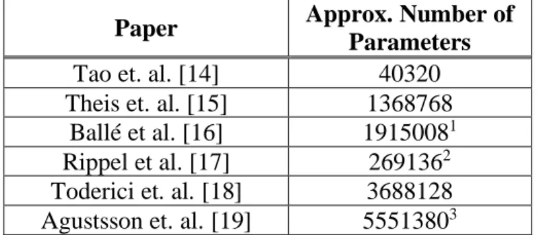
use of standard backpropagation techniques. Researchers approach this problem in various ways. In [15], the authors employ an autoencoder structure and train on the rate-distortion tradeoff loss function, replacing the derivative of the quantization function with the identity. [16] uses a similar codec structure of a nonlinear analysis transform, quantizer, and synthesis transform. However, in the analysis and synthesis transforms, convolutional filters followed by a generalized divisive normalization (GDN) joint nonlinearity are used. To overcome the non-differentiability of quantization during backpropagation, they replace quantization with additive uniform noise. In [17], the authors use a pyramidal decomposition for feature extraction and adaptive arithmetic coding with code-length regularization. In training, they use a unique generative adversarial network (GAN) formulation featuring both reconstruction and discriminator loss. Other than CNNs, different neural-network architectures have also been proposed for portions of the encoder and/or decoder, including recurrent neural networks (RNNs) and GANs. The framework of [18] uses an encoder, binarizer, and decoder where the encoder and decoder use RNN units for progressively better reconstructions. For extremely low bitrate compression, the authors of [19] use the generator network of a GAN as the decoder. With a standard convolutional encoder and quantizer, they train the full encoder-decoder pipeline by constraining the typical GAN optimization objective with both the reconstruction loss and the entropy of the encoded bitstream. For this paper, in CNN-JPEG, we employ the architecture described in [14] but modify and tune the training scheme for satellite imagery to account for observed training instabilities. The rationale for this architecture selection is that the complexity of the encoder was the smallest among the surveyed architectures. The encoder complexity generally scales with respect to execution time and memory footprint, and therefore, lower complexity designs are more feasible for deployment on embedded computers. Table 1 compares the approximate number of parameters

in the encoders for each of the surveyed methods. For the architecture in [14], the encoder, denoted ComCNN, is a 3-layer CNN that learns a compact image representation that is half the size of the original image. The compact representation is then encoded with a standard compression codec, allowing developers to incorporate any suitable lossy compression codec for their requirements. However, for this research, we employed JPEG to facilitate development due to its native integration in the TensorFlow API. Upon decoding the compact representation learned from ComCNN, the resulting image is upsampled to the original size and passed through the decoder, denoted RecCNN. Implemented with a 20-layer CNN, RecCNN reconstructs the original image by learning a residual image and adding it to the upsampled image. An alternating training scheme is employed: the decoder is first trained over an epoch of the training set with fixed encoder weights; subsequently, the encoder is trained over the same epoch with fixed decoder weights. To overcome the non-differentiability in quantization, the compression codec is removed from the pipeline in training the encoder [14].

Table 1: Approximate Number of Parameters in Encoder Network for Color Images

Paper Approx. Number of

Parameters

Tao et. al. [14] 40320

Theis et. al. [15] 1368768 Ballé et al. [16] 19150081 Rippel et al. [17] 2691362 Toderici et. al. [18] 3688128 Agustsson et. al. [19] 55513803

1 _{Assuming 192 filters for color version} 2 _{Assume 6 scales with c}

i= 64 and C=64

2.1.1 TensorFlow Lite

TensorFlow Lite4 is an open-source framework for performing on-device inference of deep-learning models applicable for a range of embedded systems. Currently, the framework contains only a subset of the operations in TensorFlow, most notably 2D convolution and matrix operations. Due to ComCNN’s simplicity, developers can port the architecture to a TensorFlow Lite model file. To accelerate inference time on ARM processors, TensorFlow Lite exercises the NEON single-instruction-multiple-data (SIMD) architecture in ARM processors. The NSF SHREC Center at the University of Pittsburgh recently examined image classification with CNNs on their CSP platform using TensorFlow Lite. More specifically, they examined CNN architectures designed for mobile applications, including MobileNetV1, MobileNetV2, Inception-ResNetV2, and NASNet Mobile, which were pre-trained on ImageNet [23].

2.1.2 Hardware Acceleration with FPGAs

Onboard inference of CNNs is computationally expensive for space platforms. Due to advances in space computers that incorporate state-of-the-art Xilinx devices, developers can use commonly available development boards as facsimiles that represent flight hardware. Many new avionics systems include hybrid SoCs with FPGAs, allowing for hardware acceleration of CNN inference. Examples include the Zynq-7020 on CSP [4], the Zynq-7030 or Zynq-7045 on SSP (and many others referenced in [3]), and the Zynq-MPSoC on SpaceCube v3.0 [5]. However, designing a custom hardware/software stack using low-level hardware description languages (HDLs) and

Linux driver development can be time consuming and non-trivial. To help alleviate this complexity and simultaneously increase productivity, Xilinx SDSoC is an integrated development environment for software-defined SoCs available for Xilinx SoCs, which can be used for rapid prototyping and development. The SDSoC design-flow abstracts many of the low-level complexities associated with developing for hybrid SoCs. As a result, developers can program their applications in C++ using compiler directives for high-level synthesis. Moreover, SDSoC allows for full-stack application development: developers can perform hardware/software partitioning by defining which functions will be accelerated on the FPGA and which will be executed directly in software on the ARM processor, with all CPU-FPGA interactions inferred.

2.2 Adaptive Compression

JPEG applies a discrete cosine transformation (DCT) on 8×8 blocks, quantizes coefficients with quantization tables tuned to a specific JPEG QF, and finally entropy encodes the quantized coefficients [20]. In our FPD-JPEG adaptive compression method, to dynamically adjust rate-distortion based upon feature content, the JPEG QF is modified according to a linear relationship with feature-point count. By adjusting the QF, we modify the quantization matrix used during encoding, allowing for increased or decreased compression at the cost of greater or lesser quantization. A low QF attempts to adjust the quantization matrix such that the high-frequency DCT components are diminished. In contrast, a high QF limits the quantization in the high-frequency DCT components, allowing for better image reconstructions.

The feature detector used in our experiments is Oriented FAST and Rotated BRIEF (ORB) [24]. ORB is commonly included in OpenCV [25] as the primary feature-point detection algorithm.

This algorithm is frequently selected due to accessibility since other competitive alternatives, such as SIFT and SURF, are not open-source and readily available.

The image-processing community has invested significant research into optimizing the quantization table in the JPEG encoder, just as FPD-JPEG attempts to do on a per-image basis. Soon after the release of the JPEG standard, the authors of [26] developed the image-dependent perceptual method, where the quantization matrix is estimated for an image that yields minimum bitrate for a given total perceptual error. As JPEG gained popularity, various optimization and search methodologies were also explored. [27] applies a recursive algorithm that seeks to optimize the quantization table by trading off the bitrate and PSNR metric. A similar approach optimizes the quantization tables using rate-SSIM graphs instead of rate-PSNR through simulated annealing [28]. Designed for one specific set of images, [29] uses an evolutionary algorithm to find specialized quantization matrices for JPEG compression of IRIS images, which lead to lower mean-square error (MSE) rates while reducing the amount of data to store. Most recently, [30] proposes a modification to the quantization table to improve PSNR at the same compression ratio by preserving more of the low-frequency DCT amplitude values.

3.0 Approach

This section describes the implementation of two compression techniques, CNN-JPEG and FPD-JPEG, for use on satellite processors. These two methods address approaches developers can exercise to supplement JPEG with other algorithms to improve compression ratio performance by adapting to the input satellite imagery. Designers can employ CNN-JPEG in missions where a sufficient amount of training data is available in order to achieve significant compression ratio gains. FPD-JPEG is easily extensible to the standard JPEG codec, essentially performing an automatic tuning of the QF based on the feature content of different images. Therefore, instead of manually tuning the QF for each image for acceptable reconstruction fidelity, FPD-JPEG can perform this functionality onboard automatically by adapting to individual input images. It is important to highlight that these methods are not restricted to JPEG alone. Rather, they can also be readily adapted to other recognized lossy compression codecs, including JPEG-2000 and BPG5_.

For CNN-JPEG, it is straightforward to replace JPEG with JPEG-2000 or BPG. To extend FPD-JPEG to other methods, one can instead tune the compression ratio parameter in FPD-JPEG-2000 or the quantizer parameter in BPG.

3.1 Compression with CNN-JPEG

As mentioned previously, CNN-JPEG follows the same neural-network architecture employed in [14]. This design features a 3-layer encoder followed by JPEG compression and 20-layer decoder. In our experiments, a JPEG QF of 50 was used. The neural-network architecture was implemented and trained in the TensorFlow framework with the JPEG encoder. To define the network in TensorFlow, two subgraphs were constructed: one to train the encoder, and one to train the decoder.

The subgraph to train the encoder features: (1) the encoder network, (2) bicubic interpolation, and (3) the decoder network. During training on this subgraph, the backward pass only updates the encoder weights. The subgraph to train the decoder features: (1) the encoder, (2) the JPEG codec, (3) bicubic interpolation, and (4) the decoder network. During training on this subgraph, the backward pass only updates the decoder weights. As with the original method, an alternating training scheme is employed, first updating the weights of the decoder over one epoch using the subgraph dedicated to training the decoder, then updating the weights of the encoder over the same epoch using the subgraph dedicated to training the decoder. After training one subgraph, the resulting updated weights for the encoder or decoder network are shared between the subgraphs.

In deep learning, hyperparameters are user-defined, high-level parameters, such as the learning rate and batch size, which the user tunes to improve model accuracy and training efficiency. To train a deep-learning model, an objective or loss function is minimized by adjusting the weights of the model typically using some form of gradient descent. With the hyperparameters and loss functions defined in [14], significant instabilities during training were observed on the training dataset comprised of satellite images. These instabilities resulted in poor reconstructions

that often had random green and yellow discolorations and spikes in intensity at various locations in the image. Figure 1 and Figure 2 show examples of these observed instabilities in the output reconstruction and the compact image representation, respectively. While the output reconstructions exhibit only a few random discolorations, the compact representations display extreme instabilities with spikes in intensity throughout the whole image. With a significant amount of random discolorations, the entropy of the compact representation is high, which increases the file size of the resulting JPEG image and results in a limited compression ratio.

Figure 1: Observed Instabilities in Output Reconstruction

Therefore, modifications were made to the training process in order to stabilize the training of the model and improve the reconstructions. Adopting the notation from [14], the CNN-JPEG encoder cost function was defined by the MSE between the reconstruction from the encoder subgraph and the original input image:

𝐿₁(𝜃₁) = 1 2𝑁∑ ‖𝑅𝑒 (𝜃̂2, 𝐶𝑟(𝜃1, 𝑥𝑘)) − 𝑥𝑘‖ 2 𝑁 𝑘=1 (3-1)

where Cr(∙) indicates inference of the encoder network with variable weights 𝜃₁, Re(∙) indicates the inference of the decoder network including bicubic interpolation with fixed weights 𝜃̂₂, 𝑥_𝑘 refers to the original input images, and N is the batch size. For the decoder, the cost function was likewise the MSE of the decoder subgraph:

𝐿2(𝜃2) = 1 2𝑁∑ ‖𝑅𝑒 (𝜃2, 𝐶𝑜 (𝐶𝑟(𝜃̂1, 𝑥𝑘))) − 𝑥𝑘‖ 2 𝑁 𝑘=1 (3-2)

where Co(∙) indicates the JPEG compression codec. Unlike Eq. 3-1, the encoder network’s weights 𝜃̂1 are fixed and the decoder network weights 𝜃2 are variable. In the original paper, this loss

function was defined in terms of the mean-square error of residual terms. Though similar, better results were observed when defining the loss function as in Eq. 3-2.

The encoder and decoder were trained on ~200,000 40×40 image patches randomly selected from the STP-H5-CSP dataset supplemented with a subset of the Berkeley dataset [31]. The STP-H5-CSP dataset consists of 489×410, 8-bit satellite images, while the Berkeley dataset consists of 8-bit natural images of random size typically in the range of 512×512. During initial experiments, the training was only performed with a subset of the STP-H5-CSP dataset. It was observed that the compression model performed well on the training subset of images, but it did not generalize well to the entire test dataset. On 28 test images, CNN-JPEG exhibited a 2.66 % increase in average PSNR and 6.20% increase in average SSIM over standard JPEG.

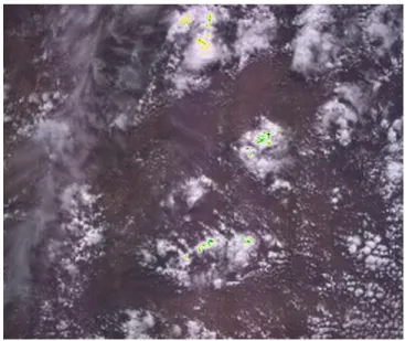
While CNN-JPEG performed well on images with few features (i.e. large portions of the image were land and/or water), it failed to reconstruct images with high-frequency features and structures not readily present in the training dataset. Figure 3 displays two examples exemplifying this model’s poor generalization to the test set. In the top image, structures such as the ISS solar panels that are infrequently present in training dataset exhibit poor visual quality in reconstruction, and in the bottom image, the finer, high-frequency structures of the clouds are blurred. Therefore, the compression model was augmented with the Berkeley dataset to learn a larger space of image structures to generalize more accurately to the test dataset. In doing so, CNN-JPEG exhibited a much larger 23.5% increase in average PSNR and 33.5% increase in average SSIM over standard JPEG.

Adam [32] is a general-purpose, state-of-the-art optimization algorithm based on gradient descent designed for training deep neural networks, adapting the learning rate for each individual trainable parameter in the model. For this design, two separate Adam optimizers were incorporated, both with parameters ∝=0.001, β1=0.9, β2=0.999, and ϵ=10-8, and were defined for

training the encoder and decoder. Unlike [14], the learning rates for the both Adam optimizers were not exponentially decayed but were fixed at 0.001, since slow convergence was observed in using decay. Additionally, we performed regularization through weight decay on both the encoder and decoder weights to stabilize training and avoid exploding gradients. This process is significant because these exploding gradients prevent convergence of the compression model and hinder reconstruction accuracy. In our experiments, the weight decays were 0.0005 for the encoder and 0.005 for the decoder.

To evaluate the compression performance of the trained model, the test images were passed through CNN-JPEG and compared with standard JPEG compression in terms of PSNR and SSIM. In the standard JPEG implementation, the JPEG QF was adjusted to achieve the same compressed file size as the trained CNN-JPEG model.

The execution time of the encoder was measured using a software timer on the ZedBoard (featuring the Zynq-7020) and ZCU102 (featuring the Zynq-MPSoC, ZU9EG) development boards, which act as facsimiles to the CSP and SpaceCube v3.0. To execute the model on the development boards, the trained encoder network weights were frozen on a standard development workstation and exported to a TensorFlow Lite model via the TensorFlow Python API. The saved model and test images were first imported using the TensorFlow Lite C++ API compiled for the ARM Cortex-A9 processors of the 7020 and the ARM Cortex-A53 processors of the

Zynq-MPSoC. Subsequently, inference was performed by invoking the TensorFlow Lite Interpreter, resulting in the compressed JPEG output file.

To decrease the execution time of the encoder, the computations in the 3-layer CNN were hardware-accelerated using the FPGA resources of the Zynq-7020 using a similar implementation to [33]. Using Xilinx SDSoC 2018.3, a hardware implementation of 2D convolution was synthesized, employing a streaming architecture where an image is streamed through the convolutional accelerator. To rapidly implement this streaming architecture, SDSoC infers multiple direct-memory access (DMA) cores with corresponding Linux device drivers, which handle the transfers of image data to and from external DDR memory. Within a single streaming convolutional unit, the 3×3 kernel multiplications with the input image occur in parallel as the image is streamed. The results of the multiplications are then summed through an adder tree to obtain the resulting pixel. Figure 4 depicts a high-level block diagram of the streaming architecture from [33]. For the Zynq-7020, the accelerator features a 2×2 grid of convolution units (Figure 5), performing four convolutions in parallel. With more FPGA resources on the Zynq-MPSoC, the convolutional grid was increased to 8×4.

Figure 5: 2×2 Grid of Convolution Units [33]

3.2 Compression with FPD-JPEG

In FPD-JPEG, the JPEG QF is adjusted based on feature-point count derived from the OpenCV implementation of ORB [25]. The hyperparameters of the ORB algorithm were first tuned to the STP-H5-CSP dataset. Specifically, for dark, featureless images, the threshold for the FAST algorithm incorporated in ORB was adjusted to ensure no features were detected. This adjustment is significant because the images on STP-H5 are collected on timed intervals and include many images taken when the ISS is over a night-covered area resulting in nearly all black pictures. In our experiments, the FAST threshold was set to 9. A maximum of 10,000 features were allowed to be detected. Once the feature points were detected, the JPEG QF was adjusted according to the linear relationship:

𝑞𝑢𝑎𝑙𝑖𝑡𝑦 𝑓𝑎𝑐𝑡𝑜𝑟 = 20(# 𝑜𝑓 𝑘𝑒𝑦𝑝𝑜𝑖𝑛𝑡𝑠

From this equation, the minimum QF is 70, whereas the maximum QF is 90 since the maximum number of features that can be detected is 10,000. For comparison, 36 representative images from the STP-H5-CSP dataset were compressed with FPD-JPEG and JPEG with static QFs of 70, 80, and 90. The average PSNR/SSIM and combined data size over the batch of images were compared between the FPD-JPEG and the static methods.

4.0 Results

This section provides a discussion of the two different methods proposed in this paper. Both techniques are compared to the original JPEG standard.

4.1 CNN-JPEG Compression

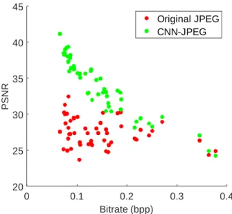
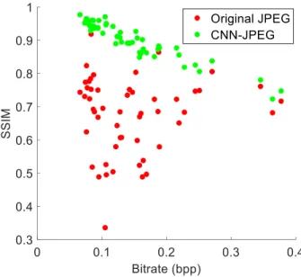
Figure 6 provides a PSNR comparison between CNN-JPEG and JPEG on a test dataset of 50 STP-H5-CSP images, while Figure 7 displays the same comparison with SSIM. On average, CNN-JPEG shows a 23.5% improved PSNR and 33.5% improved SSIM compared to JPEG images compressed to the same bitrate, measured in bits per pixel (bpp).

Figure 6: PSNR vs. Bitrate 0 0.1 0.2 0.3 0.4 Bitrate (bpp) 20 25 30 35 40 45 P S N R Original JPEG CNN-JPEG

Figure 7: SSIM vs. Bitrate

Further examination shows the PNSR/SSIM differences between CNN-JPEG and JPEG decrease as the bitrate of the image increases. For images with few features that require a lower bitrate due to low entropy in the image, CNN-JPEG significantly outperforms JPEG in both PSNR and SSIM. However, for images with more features that require a higher bitrate due to increased entropy, there is less of a difference between CNN-JPEG and JPEG. This result is expected because the rate-distortion curves tend to converge at high bitrates, achieving diminishing returns in reconstruction quality as more bits per pixel are used.

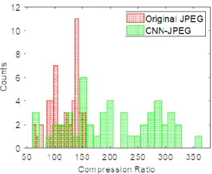
Figure 8 shows the distribution of compression ratios for the STP-H5-CSP test images when the QF is adjusted such that the JPEG-compressed images exhibit approximately the same PSNR as CNN-JPEG. The average compression ratio of CNN-JPEG is 204.36 with a standard deviation of 79.78. The average compression ratio of JPEG is 116.69 with a standard deviation of 25.59. Providing a 1.74× increase in compression ratio on average, these results show the potential benefits of using CNNs in conjunction with JPEG trained on a specific dataset. It should be

emphasized that for this dataset CNN-JPEG has a wide variation in compression performance, whereas JPEG, which is data-agnostic, will have nearly similar performance regardless of the image.

Figure 8: Distribution of Compression Ratios for Standard JPEG and CNN-JPEG

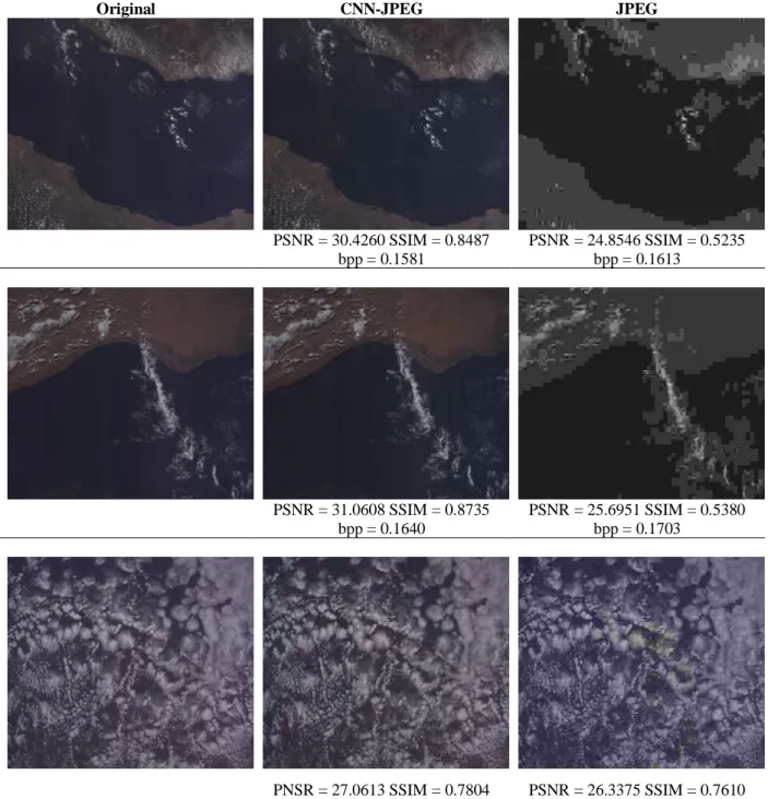
Figure 9 provides examples of three test images in the STP-H5-CSP dataset and shows a visual comparison of CNN-JPEG with JPEG. In the figure, each of the images are compressed to the same file size. This figure also demonstrates that for the same data volume, images compressed with CNN-JPEG retain more structure and detail, which would provide greater value for the data downlinked to the ground. The top and middle rows show images with relatively low entropy as large portions of the image, such as the water or land, are constant. In this low bitrate regime (~0.16 bpp for both rows), CNN-JPEG significantly outperforms standard JPEG as indicated by the 0.3252 and 0.3355 differences in SSIM in the top and middle row, respectively. In contrast, the third row shows an image with higher entropy than the top two rows as the clouds exhibit

high-frequency features in the image. For images requiring a high bitrate due to this increased entropy, the difference in reconstruction quality between CNN-JPEG and standard JPEG are less noticeable. Nonetheless, CNN-JPEG still provides more structural information than standard JPEG, indicated by the 0.7238 dB and 0.0194 increase in PSNR and SSIM, respectively.

Original CNN-JPEG JPEG PSNR = 30.4260 SSIM = 0.8487 bpp = 0.1581 PSNR = 24.8546 SSIM = 0.5235 bpp = 0.1613 PSNR = 31.0608 SSIM = 0.8735 bpp = 0.1640 PSNR = 25.6951 SSIM = 0.5380 bpp = 0.1703 PNSR = 27.0613 SSIM = 0.7804 bpp = 0.3455 PSNR = 26.3375 SSIM = 0.7610 bpp = 0.3535

Considering realistic mission scenarios, employing CNN-JPEG is advantageous primarily for lossy compression of satellite images when a system is determining what full science data products to retrieve via lossless compression. At the same file size as JPEG, CNN-JPEG provides better perceptual quality for visual inspection of the science products. Therefore, CNN-JPEG uses downlink bandwidth more efficiently, providing more information with comparatively less data. Additionally, when a satellite is not directly over a ground station or if the transceiver link is interrupted, it is always advantageous to use CNN-JPEG for file storage purposes. When the downlink is reestablished, CNN-JPEG, with its 1.74× increase in average compression ratio, will reduce the amount of data required to downlink.

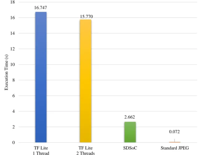
Executing the encoding portion of CNN-JPEG in TensorFlow Lite on the Cortex-A9 cores of the Zynq-7020, the average execution time with one thread was 16.75 s, as indicated in Figure 10. In changing from single-threaded to double-threaded execution via the TensorFlow Lite interpreter, the execution time was reduced only by ~1.0 s. This indicates the parallelization through the TensorFlow Lite interpreter deviates far from ideal linear speedup. Leveraging the FPGA resources of the Zynq-7020 through SDSoC for hardware acceleration, the average execution time of the CNN-JPEG encoder decreased significantly to 2.293 s, exhibiting 7.30× and 6.87× speedup over the single-threaded and double-threaded TensorFlow Lite implementations, respectively. The maximum clock frequency achieved was 100 MHz for the FPGA fabric. The limiting critical path in the design is the write DMAs for output buffers. Similarly, the design was also executed on the Zynq-MPSoC with the results indicated in Figure 11. For the Zynq-MPSoC, there was a reduction of ~0.6 s from single-threaded to quad-threaded execution. For the hardware-accelerated implementation, the design saw a 15.57× and 11.11× speedup over the single-threaded

and quad-threaded runs, respectively. Comparing with standard JPEG, the CNN-JPEG execution time shows a 36.97× and 4.25× increase on the Zynq-7020 and Zynq-MPSoC respectively, which is expected due to the increased number of computations. However, despite this increase in execution time, CNN-JPEG can make extensive use of transceiver link downtime to produce science data products with better visual quality at the same or better data rate as JPEG. Future improvements to CNN-JPEG will attempt to decrease execution time through fixed-point quantization of the encoder network weights. The resource utilization for the hardware acceleration portion of the model is shown in Table 2.

Figure 10: Execution Time on Zynq-7020 16.747 15.770 2.662 0.072 0 2 4 6 8 10 12 14 16 18 TF Lite 1 Thread TF Lite 2 Threads

SDSoC Standard JPEG

E xe cut io n T im e (s )

Figure 11: Execution Time on Zynq-MPSoC 2.118 1.512 0.136 0.032 0 0.5 1 1.5 2 2.5 TF Lite 1 Thread TF Lite 4 threads

SDSoC Standard JPEG

E xe cut io n T im e (s )

Table 2: Resource Utilization Resource Zynq-7020 (100 MHz) Zynq-MPSoC (ZU9EG; 300 MHz) CLB LUTs 78.48% 64.67% CLB FF 58.81% 55.82% BRAM/FIFO ECC (36 Kb) 40.00% 14.75% DSP Slices 88.64% 60.12 %

The average dynamic power was also recorded for these algorithms using a Watts Up power meter on both the Zynq-7020 and Zynq-MPSoC for each of the implementations described, as shown in Figure 12 and Figure 13, respectively. The average dynamic power was calculated by subtracting the idle power of the development board from the average power consumed during program execution. As expected, both SDSoC implementations of CNN-JPEG draw significantly more dynamic power than their corresponding TensorFlow Lite software implementations due to the use of the FPGA resources on the SoC. With a 2×2 convolutional grid running at 100 MHz on the Zynq-7020, the SDSoC design consumed 2.10× and 5.10× more dynamic power than the double-threaded and single-threaded TensorFlow Lite programs, respectively. In contrast, with an 8×4 convolutional grid running at 300 MHz on the Zynq-MPSoC, the SDSoC design consumed 3.37× and 6.80× more dynamic power than the single-threaded and double-threaded TensorFlow Lite programs, respectively. Due to the higher clock frequency and increased FPGA resource usage, the Zynq-MPSoC SDSoC design shows a relative increase in dynamic power in comparison to the Zynq-7020. Comparing these CNN-JPEG implementations with standard JPEG, the average dynamic power of standard JPEG is smaller than all CNN-JPEG implementations on both the

Zynq-7020 and Zynq-MPSoC. Specifically, on the Zynq-7020, the single-threaded TensorFlow Lite and SDSoC implementations drew 1.12× and 5.72× more dynamic power than standard JPEG, respectively. On the Zynq-MPSoC, the single-threaded TensorFlow Lite and SDSoC implementations drew 2.26× and 15.4× more dynamic power than standard JPEG, respectively. These results illustrate the design tradeoffs to be examined by mission developers: CNN-JPEG provides significant improvements in storage volume, but it requires compromises in execution time and power usage when compared to standard JPEG.

Figure 12: Dynamic Power on Zynq-7020 0.146 0.354 0.744 0.130 0 0.1 0.2 0.3 0.4 0.5 0.6 0.7 0.8 TF Lite 1 Thread TF Lite 2 Threads

SDSoC Standard JPEG

D y n a m ic P o w er (W )

Figure 13: Dynamic Power on Zynq-MPSoC 0.496 1.000 3.373 0.219 0 0.5 1 1.5 2 2.5 3 3.5 4 TF Lite 1 Thread TF Lite 4 Threads

SDSoC Standard JPEG

D y n a m ic P o w er (W )

4.2 FPD-JPEG Compression

Figure 14 and Figure 15 show the average PSNR and SSIM respectively of the FPD-JPEG compared with JPEG at static QFs over the dataset of 36 representative STP-H5-CSP images. Based on the linear relationship defined in Eq. 3-3, the QF for FPD-JPEG ranges from 70 to 90. Therefore, for comparison, static QFs of 70, 80, and 90 for JPEG were chosen to demonstrate how combined file size and PSNR/SSIM scale over the same QF range as FPD-JPEG. Comparing FPD-JPEG with standard JPEG at static QF=90, the average PSNR and SSIM over the batch decreased by only 0.172 dB and 0.0017, respectively. However, the combined file size accumulated over the 36 encoded images was considerably reduced by 29.6%. In addition, the combined file size of FPD-JPEG was only 10.3% higher than the static JPEG QF=80 but provides a 1.894 dB increase in PSNR and 0.0113 increase in SSIM.

Figure 14: FPD-JPEG Compression SSIM Comparison 0 200 400 600 800 1000 1200 1400 1600 0.945 0.95 0.955 0.96 0.965 0.97 0.975 0.98

Static QF=70 Static QF=80 Static QF=90 FPD-JPEG

Co m b in ed F il e S iz e (kB ) A v er age S S IM

Figure 15: FPD-JPEG Compression PSNR Comparison 0 200 400 600 800 1000 1200 1400 1600 35 36 37 38 39 40 41

Static QF=70 Static QF=80 Static QF=90 FPD-JPEG

Co m b in ed F il e S iz e (kB ) A v er a ge P S N R

These increases in PSNR and SSIM between FPD-JPEG and standard JPEG at a static QF=80 can be significant in terms of visual quality, particularly when examining the distinct edges of coastlines in an image. To highlight the importance of these increases in PSNR and SSIM,

Figure 16 shows a comparison of two cropped images zoomed in on the coastline in the same ~1.9 dB PSNR and ~0.01 SSIM difference range as FPD-JPEG and JPEG with static QF=80. Since JPEG operates over 8×8 blocks in an image, it can distort or introduce block artifacts into the image, which become particularly apparent when examining the coastline. In this example, the bottom image, with its 1.940 dB increase in PSNR and 0.0099 increase in SSIM, exhibits a sharper coastline edge with less block artifacts as compared to the top image.

PSNR = 37.8478 SSIM = 0.9661

PSNR = 39.7874 SSIM =0.9760

The average execution time for FPD-JPEG and standard JPEG are shown in Figure 17 and Figure 18 for the Zynq-7020 and for the Zynq-MPSoC, respectively. On the Zynq-7020, FPD-JPEG shows a 5.58× increase in execution time as compared to standard FPD-JPEG. On the Zynq MPSoC, FPD-JPEG shows a 3.52× increase in execution time as compared to standard JPEG. The average dynamic power for both algorithms was also measured: for the Zynq-7020, the average dynamic power for both algorithms was 0.18 W, and for the Zynq-MPSoC, the average dynamic power was likewise 0.18 W.

Figure 17: FPD-JPEG Execution Time on Zynq-7020 0.134 0.024 0 0.02 0.04 0.06 0.08 0.1 0.12 0.14 0.16

FPD-JPEG Standard JPEG

E xe cut io n T im es (s )

Figure 18: FPD-JPEG Execution Time on Zynq-MPSoC 0.074 0.021 0 0.01 0.02 0.03 0.04 0.05 0.06 0.07 0.08

FPD-JPEG Standard JPEG

E xe cut io n T im e (s )

For a mission designer, these results indicate that FPD-JPEG is a relatively simple extension for systems with JPEG already baselined. For a slight increase in execution time and power, FPD-JPEG can conserve nearly a third of the data volume with minimal concessions to image quality compared with JPEG using a static QF=90. Moreover, unlike CNN-JPEG, FPD-JPEG uses a classical computer-vision algorithm without the need to train a neural network. Therefore, since FPD-JPEG requires only the addition of ORB functions while CNN-JPEG requires training and the addition of TensorFlow Lite libraries, it may be less intrusive and less resource-intensive to current onboard systems already using JPEG (or another codec that this method can tune) in comparison to CNN-JPEG.

5.0 Conclusions

This research examined two lossy image-compression methods that serve to supplement JPEG for onboard processing systems: the first, CNN-JPEG, adopts the CNN architecture of [14] trained on satellite images, while the second, FPD-JPEG, uses an adaptive approach that fine-tunes the JPEG QF based on feature-point content to achieve combined file size reductions over a batch of images. Experimental results for CNN-JPEG show a 23.5% and 33.5% increase in PSNR and SSIM over standard JPEG, respectively, on an image dataset collected from STP-H5-CSP compressed to the same file size. On the same dataset, CNN-JPEG showed a 1.74× increase in average compression ratio at the same PSNR. We demonstrated substantial performance benefits through hardware acceleration of the TensorFlow Lite implementation of the encoder using Xilinx SDSoC. This hardware-accelerated design demonstrated an immense speedup of over 6.87× on the Zynq-7020 and over 11.11× on the Zynq-MPSoC enabling feasible deployment on a satellite platform. Therefore, Xilinx SDSoC proved to be an efficient framework for rapid development of hardware-accelerated designs for CNN inference. For FPD-JPEG, experimental results indicate that fine-tuning the JPEG QF using a linear relationship with feature-point count achieves a less than 1% drop in average PSNR and SSIM while reducing the combined file size by 29.6% when compared to a static QF=90 over a batch of satellite images collected on STP-H5-CSP. As a result, FPD-JPEG provides nearly the same average visual quality as JPEG with static QF=90 over a batch of images while vastly decreasing the amount of data that needs to be stored and transmitted to the ground.

6.0 Future Work

This research provides a compelling starting point for evaluating the latest state-of-the-art compression techniques for onboard systems, instead of defaulting to less effective heritage techniques. There are numerous extensions that could be pursued to provide solutions more broadly applicable to more satellite systems and sensor instruments.

For CNN-JPEG, the first extension is to study higher QFs used to compress the compact representation (greater than 50, as in the above experiments) of the image in order to measure the difference in distortion between JPEG at higher bitrates. Additionally, this neural network architecture can be extended to other codecs such as JPEG-2000 and BPG whose reconstruction fidelities at lower bit rates are often better than JPEG. Since TensorFlow does not currently support JPEG-2000 or BPG in their graph API, an external API must be used in conjunction with TensorFlow.

For faster encoding execution times, the encoder neural-network model will be quantized to use fixed-point integer arithmetic instead of floating-point for both the TensorFlow Lite software implementation and the hardware-accelerated SDSoC version. However, this quantization may come at the cost of reconstruction accuracy. Therefore, we will examine quantitatively how PSNR and SSIM loss occurs from quantizing just the encoding portion of CNN-JPEG.

Beyond CNN-JPEG, we will examine other machine-learning models with more complex encoders to provide potentially improved compression ratios. One of the primary focuses of this study will be to determine how much speedup can be obtained via hardware-acceleration of the

encoder such that their execution times are fast enough to sustain real-time or near real-time encoding with large bandwidth sensors.

Both CNN-JPEG and FPD-JPEG will be deployed on NSF SHREC experiments currently operating on the ISS, namely STP-H5-CSP and STP-H6-SSIVP. A study will be conducted to profile the bandwidth savings in a relevant mission scenario. For CNN-JPEG, the TensorFlow Lite version will first be uploaded to demonstrate functionality. Once this demonstration is complete, a bit stream for the convolutional accelerator will then be uploaded to reconfigure the FPGA.

Bibliography

[1] T. M. Lovelly and A.D. George, “Comparative Analysis of Present and Future Space-Grade Processors with Device Metrics,” AIAA J. of Aerospace Inf. Syst., vol. 14, no. 3, pp. 184-197, Mar. 2017.

[2] 2015 NASA Technology Roadmaps, Washington, D.C., USA: NASA Office of the Chief Technologist, 2015. [Online]. Available: https://www.nasa.gov/offices/oct/ home/roadmaps/index.html

[3] A. D. George and C. Wilson, “Onboard Processing with Hybrid and Reconfigurable Computing on Small Satellites,” Proc. of the IEEE, vol. 106, no. 3, pp. 458-470, Mar 2018. [4] C. Wilson and A. D. George, “CSP: Hybrid Space Computing,” AIAA J. of Aerospace Inf.

Syst., vol. 15, no. 4, pp. 215–227, Feb 2, 2018. doi: https://doi.org/ 10.2514/1.I010572 [5] A. Geist, C. Brewer, M. Davis, N. Franconi, S. Heyward, T. Wise G. Crum, D. Petrick, R.

Ripley, C. Wilson, and T. Flatley, “SpaceCube v3.0 NASA Next-Generation High-Performance Processor for Science Applications,” 33rd Annu. AIAA/USU Conf. on Small Satellites, SSC19-XII-02, Logan, UT, August 3-8, 2019.

[6] NASA Space Technology Roadmaps and Priorities, Washington, D.C., USA: National Academy Press, 2012. [Online]. Available: https://www.nap.edu /catalog/23582/nasa-space-technology-roadmaps-and-priorities-revisited

[7] NASA Space Technology Roadmaps and Priorities Revisited, Washington, D.C., USA: National Academy Press, 2016. [Online]. Available: https://www.nap.edu /catalog/23582/nasa-space-technology-roadmaps-and-priorities-revisited

[8] Thriving on Our Changing Planet A Decadal Strategy for Earth Observation from Space, Washington, D.C., USA: National Academy Press, 2018. [Online]. Available: https://www.nap.edu/catalog/24938/thriving-on-our-changing-planet-a-decadal-strategy-for-earth

[9] C. Mercer, “Small Satellite Missions for Planetary Science,” 33rd Annu. AIAA/USU Conf. on Small Satellites, SSC19-WKV-06, Logan, UT, August 3-8, 2019.

[10] B. Lal, E. de la Rosa Blanco, J. R. Behrens, B. A. Corbin, E. K. Green, A. J. Picard, and A. Balakrishnan, “Global Trends in Small Satellites,” IDA Paper P-8638, 2017.

[11] Compressive Sensing for DoD Sensor Systems, McLean, Virginia, USA: JASON, 2012. [Online]. Available: https://fas.org/irp/agency/dod/jason/compres s.pdf

[12] N. D. Beser, “Space Data Compression Standards,” John Hopkins APL Technical Digest, vol. 15, no. 3, pp. 206-223, 1994.

[13] G. Yu, T. Vladimirova, and M. Sweeting, “Image compression systems on board satellites,” in Acta Astronautica, vol. 64, pp. 988-1005, 2009.

[14] W. Tao, F. Jiang, S. Zhang, J. Ren, W. Shi, W. Zuo, X. Guo, and D. Zhao, "An End-to-End Compression Framework Based on Convolutional Neural Networks," in Data Compression Conf. (DCC), Snowbird, UT, Apr. 4-7, 2017.

[15] L. Theis, W. Shi, A. Cunningham, and F. Huszár, "Lossy Image Compression with Compressive Autoencoders," in International Conference on Learning Representations (ICLR), Toulon, France, Apr. 24-26, 2017.

[16] J. Ballé, V. Laparra, and E. P. Simoncelli, “End-to-end Optimized Image Compression,” in

International Conference on Learning Representations (ICLR), Toulon, France, Apr. 24-26, 2017.

[17] O. Rippel and L. Bourdev, "Real-Time Adaptive Image Compression," in International Conference on Machine Learning, Sydney, Australia, Aug. 7-9, 2017.

[18] G. Toderici, D. Vincent, N. Johnston, S. Jin Hwang, D. Minnen, J. Shor, and M. Covell, “Full Resolution Image Compression with Recurrent Neural Networks,” in 2017 IEEE Conference on Computer Vision and Pattern Recognition (CVPR), Honolulu, HI, Jul. 21-26, 2017.

[19] E. Agustsson M. Tschannen, F. Mentzer, R. Timofte, L. V. Gool, “Generative Adversarial Networks for Extreme Learned Image Compression,” in International Conference on Computer Vision (ICCV), Seoul, Korea, Oct. 27-Nov. 2, 2019.

[20] G. K. Wallace, "The JPEG still picture compression standard," in IEEE Trans. on Consum. Electronics, vol. 38, no. 1, pp. xviii-xxxiv, Feb. 1992.

[21] A. Skodras, C. Christopoulos and T. Ebrahimi, "The JPEG 2000 still image compression standard," in IEEE Signal Process. Mag., vol. 18, no. 5, pp. 36-58, Sept. 2001.

[22] Z. Wang, A. C. Bovik, H. R. Sheikh, and E. P. Simoncelli, "Image quality assessment: from error visibility to structural similarity," in IEEE Trans.on Image Process., vol. 13, no. 4, pp. 600-612, April 2004.

[23] J. Manning, D. Langerman, B. Ramesh, E. Gretok, C. Wilson, A. D. George, J. MacKinnon, G. Crum, “Machine-Learning Space Applications on SmallSat Platforms with TensorFlow,”

32nd Annu. AIAA/USU Conf. on Small Satellites, SSC18-WKVII-03, Logan, UT, Aug 4-9, 2018.

[24] E. Rublee, V. Rabaud, K. Konolige, and G. Bradski, “ORB: An efficient alternative to SIFT or SURF,” in Proc. of 2011 Int. Conf. on Comput. Vision, Barcelona, Spain, Nov. 6-13, 2011. [25] G. Bradski, "The opencv library," Dr Dobb's J. Software Tools, vol. 25, pp. 120-125, 2000. [26] A. B. Watson, “Visual Optimization of DCT Quantization Matrices for Individual Images,”

in Proc. AIAA Comput. in Aerosp. San Diego, CA, American Institute of Aeronautics and Astronautics, vol. 9, pp. 286-291, 1993.

[27] S. W. Wu and A. Gersho, "Rate-constrained picture-adaptive quantization for JPEG baseline coders," in IEEE Int. Conf. on Acoust., Speech, and Signal Process., Minneapolis, MN, Apr 27-30, 1993.

[28] Y. Jiang and M. S. Pattichis, "JPEG image compression using quantization table optimization based on perceptual image quality assessment," in 2011 Conf. Rec. of the Forty Fifth Asilomar Conf. on Signals, Systs. and Comput. (ASILOMAR), Pacific Grove, CA, Nov. 6-9, 2011.

[29] M. Konrad, H. Stogner, and A. Uhl, "Evolutionary Optimization of JPEG Quantization Tables for Compressing Iris Polar Images in Iris Recognition Systems," in 2009 Proc. of 6th Int. Symp. on Image and Signal Process. and Anal., Salzburg, Austria, Sep. 16-18, 2009. [30] L. Alam, K. Dhar, M. A. F. M. Rashidul Hasan, M. Golam, S. Bhuyan, and G. Daiyan, “An

Improved JPEG Image Compression Algorithm by Modifying Luminance Quantization Table,” Int. J. of Comput. Sci. and Netw. Secur, vol. 17, no. 1, pp. 200-208, Jan. 2017. [31] The Berkeley Segmentation Dataset and Benchmark. Berkeley, CA, USA: Computer Vision

Group. [Online]. Available: https://www2.eecs.berkeley.edu/Research/ Projects/CS/vision/bsds/

[32] D. P. Kingma and J. Ba, “Adam: A method for stochastic optimization,” in International Conference on Learning Representations (ICLR), San Diego, CA, May 7-9, 2015.

[33] S. Sabogal, A. D. George, and G. Crum, “ReCoN: Reconfigurable CNN Acceleration for Space Applications A Framework for Hybrid Semantic Segmentation on Hybrid SoCs,” 12th Space Computing Conf., Jul. 30 – Aug. 1, 2019.