Title
Three Essays on Vulnerable Workers Permalink https://escholarship.org/uc/item/1w28961w Author Bana, Sarah H Publication Date 2019 Peer reviewed|Thesis/dissertation
Three Essays on Vulnerable Workers
A dissertation submitted in partial satisfaction of the requirements for the degree
Doctor of Philosophy in Economics by Sarah H. Bana Committee in charge:
Professor Peter Kuhn, Chair Professor Kelly Bedard Professor Heather Royer
Professor Kelly Bedard
Professor Heather Royer
Professor Peter Kuhn, Committee Chair
Copyright c 2019 by
Sarah H. Bana
This dissertation would not be the same without the direction and support of my committee. I am deeply indebted to my advisor, Peter Kuhn, for his thoughtful comments on each and every draft of my first essay. His clarity of thought, thorough knowledge of the literature and relentless pursuit to improve our understanding of the world guided my approach to research. He has shown me, by example, what a good economist (and person) should be. Kelly Bedard has been an extraordinary mentor and co-author. The incredible opportunity she gave me to work on important research lead to my second and third essays. Her lessons in how to think about data and the stories it is telling us have made me a better researcher. Heather Royer believed in me early on and set high standards for me. Her family gave me a sense of belonging in Santa Barbara, which was instrumental to my success.
The terrific environment in the UCSB Economics department made it a wonderful place to work on my dissertation. I am immensely grateful to the faculty and students who supported my work. My graduate student mentor and now co-author, Jenna Stearns, provided insights from across the hall at all hours of the day. Cathy Weinberger gave thoughtful feedback and encouragement on presentations and drafts. I took full advantage of Shelly Lundberg and Dick Startz’s open door policy. Maya Rossin-Slater has been a great co-author. My officemates, Max Lee and Levi Marks, were my friends in the trenches. My housemate, Lizi Yu, would listen to my research updates, morning and night. The rest of my cohortmates– Yuan Cao, Michael Cooper, Zheng Wang, and Andrew Ayres– helped me create a positive cohort culture. Matt Wibbenmeyer was enthusiastic about my research at every stage. Beyond UCSB, members of my broader economics cohort– Mackenzie Alston, Britta Glennon, Do Yoon Kim and Daniel Rock– empowered me and gave me a broader sense of community. Everyone was extremely
moments, my parents reminded me that success does not come quickly or easily. My sister was my personal cheerleader, celebrating every accomplishment along the way. My brother listened thoughtfully when I spoke about research. Ali Merali inspired me to sharpen my thinking. Aliya Bhimani let me know when I was too hard on myself. My DC friends gave me a home away from home and a sense that all the work was worth it. My AKEB friends celebrated the knowledge discovery I engaged in every day. This dissertation would have not been possible without the investment of these amazing individuals.
Ph.D. Economics, University of California, Santa Barbara, 2019
M.A. Economics, University of California, Santa Barbara, 2014
M.A. Applied Economics, Georgetown University, 2013
B.A. Quantitative Economics, University of California, Irvine, 2010
F S
Labor economics and applied econometrics
W P
Identifying Vulnerable Displaced Workers: The Role of State-Level Occupation Conditions
Media Coverage:Wall Street Journal – Real Time Economics Blog
The Impact of Paid Family Leave Benefits: Regression Kink Evidence from California Ad-ministrative Data with Kelly Bedard and Maya Rossin-Slater
• Available as NBER Working Paper No. 24438 and IZA Discussion Paper No. 11381 Unequal Use of Social Insurance: The Role of Employers with Kelly Bedard, Maya Rossin-Slater and Jenna Stearns
• Available as NBER Working Paper No. 25163 and IZA Discussion Paper No. 11882
P
Bana, Sarah, Kelly Bedard, and Maya Rossin-Slater. 2018. “Trends and Disparities in Leave Use under California’s Paid Family Leave Program: New Evidence from Administrative Data.”AEA Papers & Proceedings, 108: 388-91.
F
Research Awards – External
2017 $10,000 award from the Workforce Data Initiative at the University of
Chicago’s Center for Data Science and Public Policy (funded by the Alfred P. Sloan Foundation)
Research Awards – Internal
2018 Division of Social Sciences Fellowship
2017 Professor Robert T. Deacon Graduate Fellowship in Economics
2013 Economics Department Block Grant Fellowship
Teaching Awards – Internal
2018 UCSB Economics Outstanding Teaching Assistant of the Quarter (for Fall
2017 – Introduction to Econometrics) Travel Grants – Internal
2018 UCSB Academic Senate Doctoral Student Travel Grant
2017 UCSB Economics Graduate Student Travel Grant
2016 Dean’s Grant for ICPSR Training
DFG Conference on Technology, Demographics and the Labor Market – Cologne, Germany (March 2019)
Southern Economic Association Conference – Washington, DC (November 2018) WEAI Graduate Student Workshop – Vancouver, BC (June 2018)
APPAM Regional Student Conference – Washington, DC (May 2018) WEAI Annual Conference – San Diego, CA (June 2017)
Society of Labor Economists (SOLE) Conference – Raleigh, NC (May 2017)
P P
All California Labor Economics Conference – University of Southern California (October 2018)
Summer School on Socioeconomic Inequality – University of Chicago (July 2016)
I T
University of Memphis (January 2019) RAND Corporation (January 2019) U.S. Census Bureau (January 2019) Bureau of Labor Statistics (January 2019) Colby College (January 2019)
Carleton University (January 2019)
T E
Instructor of Record
Economics 140A: Introduction to Econometrics Teaching Assistant
Economics 140B: Introduction to Econometrics Economics 140A: Introduction to Econometrics Economics 10A: Microeconomic Theory Economics 1: Principles of Microeconomics
W P
6th Lindau Meeting on Economic Sciences (funded by the National Science Foundation) ICPSR Workshop on Machine Learning: Applications and Opportunities in the Social Sci-ences
NBER Economics of Digitization Graduate Student Tutorial Summer School on Socioeconomic Inequality
R A E
Research assistant for Prof. Heather Royer (2014-2017) Research assistant for Prof. Shelly Lundberg (2015) Research assistant at the RAND Corporation (2010-2013)
Three Essays on Vulnerable Workers by
Sarah H. Bana
Vulnerable workers, workers who have recently experienced a shock that could adversely affect their labor market prospects, experience large, long-lasting earnings losses – on average. This dissertation investigates the mechanisms behind the losses of three groups of vulnerable workers and the role of public policy in mitigating these losses. In the first essay, I identify which displaced workers, workers who lose their job as a result of a firm or plant closing, are the most vulnerable. I find that a worker’s duration of joblessness depends much more on conditions within that worker’s occupation than conditions within that worker’s industry. This suggests a worker’s vulnerability is a function of their skills and less related to the goods and services they were previously producing. In the second essay, my collaborators and I estimate the causal impacts of benefits in California’s Paid Family Leave program on a second group of vulnerable workers: new mothers. We find no evidence that a higher weekly benefit amount increases leave duration or leads to adverse future labor market outcomes for mothers with earnings near the maximum benefit threshold. In the third essay, my collaborators and I find strong evidence that Disability Insurance and Paid Family Leave program take-up is substantially higher in firms with high earnings premiums. Our results suggest that changes in firm behavior have the potential to impact social insurance use and thus reduce an important dimension of inequality in America.
Abstract ix
1 Introduction 1
1.1 Permissions and Attributions . . . 3
2 Identifying Vulnerable Displaced Workers: The Role of State-Level Occupation Conditions 5 2.1 Introduction . . . 5 2.2 Data . . . 10 2.3 Empirical Approach . . . 14 2.4 Results . . . 22 2.5 Robustness . . . 29 2.6 Conclusion . . . 36
3 The Impact of Paid Family Leave Benefits: Regression Kink Evidence from California Administrative Data 57 3.1 Introduction . . . 57
3.2 Background on CA-PFL and the Benefit Schedule . . . 64
3.3 Data and Sample . . . 66
3.4 Empirical Design . . . 69
3.5 Results . . . 76
3.6 Conclusion . . . 83
4 Unequal Use of Social Insurance: The Role of Employers 95 4.1 Introduction . . . 95
4.2 Temporary Social Insurance in California . . . 100
4.3 Data . . . 103
4.4 Empirical Strategy . . . 108
4.5 Results . . . 113
4.6 Conclusion . . . 122
B Appendix for Unequal Use of Social Insurance: The Role of Employers 151 B.1 Appendix Tables . . . 151
Introduction
This dissertation contains three essays on vulnerable workers, workers who have recently experienced a shock that could adversely affect their labor market prospects. Each chapter explores the mechanisms behind vulnerable workers’ earnings losses and the role of public policy in mitigating these losses. I identify important factors in workers’ labor market success, shedding light on the earnings determination process. With a better understanding of relevant factors, I assess whether state programs are allocating resources to the most vulnerable workers.
In the first essay, I study displaced workers, workers who lose their job as a result of a firm or plant closing. On average, displaced workers experience large, long-lasting earnings losses, but some displaced workers experience larger earnings changes after displacement than others. I use comprehensive occupational employment data to estimate the effect of the state-level occupation growth rate in the worker’s pre-displacement occupation on subsequent labor market outcomes. I find that adverse labor market conditions in a worker’s occupation at the time of displacement have negative consequences. Displacement from a shrinking occupation is associated with decreased earnings and longer durations of joblessness. Furthermore, holding the occupation growth rate constant,
there is only a small effect of the worker’s industry growth rate on their labor market outcomes. These results suggest that vulnerable displaced workers’ difficulties in the labor market are a function of their skills and less related to the goods and services they were previously producing. The workers at greatest risk have occupation specific human capital that is less valuable after their job loss, leading to either longer durations of joblessness or larger earnings losses.
Displaced workers are not the only workers who experience sizable and persistent earnings losses. More recently, researchers have found a similar profile of losses amongst mothers after the birth of their first child. It appears job displacement is not the only major life event with labor market consequences. The second essay investigates the effect of additional benefits on mothers who have new family responsibilities in California’s Paid Family Leave program.
Specifically, with my co-authors Kelly Bedard and Maya Rossin-Slater, I use ten years of California administrative data with a regression kink design to estimate the causal impacts of benefits in the first state-level paid family leave program for women with earnings near the maximum benefit threshold. We find no evidence that a higher weekly benefit amount (WBA) increases leave duration or leads to adverse future labor market outcomes for this group. In contrast, we document that a rise in the WBA leads to an increased likelihood of returning to the pre-leave firm (conditional on any employment) and of making a subsequent paid family leave claim.
The Paid Family Leave (PFL) program in California falls under the larger umbrella of State Disability Insurance. PFL and Disability Insurance (DI) have become important sources of social insurance, with benefit payments now exceeding those of the state’s Unemployment Insurance program. However, there is considerable inequality in program take-up. While existing research shows that firm-specific factors explain a significant part of the growing earnings inequality in the U.S., little is known about the role of firms
in determining the use of public leave-taking benefits.
In the third essay, using administrative data from California with my co-authors Kelly Bedard, Maya Rossin-Slater, and Jenna Stearns, I find strong evidence that DI and PFL program take-up is substantially higher in firms with high earnings premiums. A one standard deviation increase in the firm premium is associated with a 57 percent higher claim rate incidence. Put differently, take-up of temporary social insurance programs is lower in lower earnings premium firms. Workers at these firms, therefore, are more vulnerable from both an earnings perspective and a benefits perspective. Our results suggest that changes in firm behavior have the potential to impact social insurance use and thus reduce an important dimension of inequality in America. Despite near-universal program eligibility for workers, non-policy-driven determinants of take-up play a major role.
1.1
Permissions and Attributions
Peter Kuhn provided valuable guidance in the work leading to Chapter 2. This chapter also benefited from helpful comments from Kelly Bedard, Heather Royer, Cathy Weinberger, Jenna Stearns, Jim Spletzer and Elizabeth Handwerker, as well as members of the UCSB Human Capital Working Group, the Bureau of Labor Statistics, the Census Bureau, and participants at the Summer School on Socioeconomic Inequality 2016, Society of Labor Economics Meetings 2017, and Southern Economics Association 2018.
Chapter 3 is the result of a collaboration with Kelly Bedard and Maya Rossin-Slater. In the course of writing this chapter, we benefited from the comments of Clement de Chaisemartin, Yingying Dong, Peter Ganong, Simon Jaeger, Zhuan Pei, Lesley Turner, and seminar and conference participants at UCSB, UC Berkeley (Haas), University of Notre Dame, Brookings Institution, the Western Economic Association International
(WEAI), the National Bureau of Economic Research (NBER) Summer Institute, the “Child Development: The Roles of the Family and Public Policy” conference in Vejle, Denmark, the All-California Labor Economics Conference, the ESSPRI workshop at UC Irvine, and the Southern Economic Association meetings for valuable comments. Rossin-Slater is grateful for support from the National Science Foundation (NSF) CAREER Award No. 1752203. Any opinions, findings, and conclusions or recommendations expressed in this paper are those of the authors and do not necessarily reflect the views of the National Science Foundation. The California Employment Development Department (EDD) had the right to comment on the results of the paper, per the data use agreement between the authors and the EDD.
Chapter 4 is the result of a collaboration with Kelly Bedard, Maya Rossin-Slater and Jenna Stearns. We thank Kent Strauss for valuable research assistance. In the course of writing this chapter, we benefited from the comments of Isaac Sorkin, as well as seminar participants at the University of Toronto, the All-California Labor Economics conference and the AEA meetings for helpful comments. Rossin-Slater is grateful for support from the National Science Foundation (NSF) CAREER Award No. 1752203. Any opinions, findings, and conclusions or recommendations expressed in this paper are those of the authors and do not necessarily reflect the views of the National Science Foundation. The California Employment Development Department (EDD) had the right to comment on the results of the paper, per the data use agreement between the authors and the EDD.
Identifying Vulnerable Displaced
Workers: The Role of State-Level
Occupation Conditions
2.1
Introduction
Displaced workers, workers who lose their job as a result of a firm or plant closing, have large earnings losses on average. However, these large average losses mask substantial variation across workers. What explains this variation? Prior research shows that workers displaced when the national unemployment rate is high experience larger earnings losses than those displaced when the national unemployment rate is low. But the national unemployment rate may mask substantial differences between workers in their labor market prospects. Specifically, a worker may have more or less difficulty finding work depending on conditions in their occupation, defined as the set of activities or tasks they are paid to perform, or their industry, defined as the primary business activity of their establishment. The roles of these pre-displacement employment attributes may shed
light on the circumstances under which a worker’s human capital may be less valuable. This distinction is also important to effectively target job search assistance to recently unemployed workers.
Attempts to perform such an analysis have been constrained by data limitations. Specifically, because occupation is a worker-level characteristic with many options, annual occupational employment estimates to measure short-term employment fluctuations do not exist in the United States. I address this limitation by constructing a novel measure of occupation conditions that captures short-term state-level fluctuations in occupational employment by combining existing datasets on the share of each occupation in an industry and industry growth rates.
I then use data from the Current Population Survey Displaced Worker Supplement to study the effects of poor state labor market conditions in a displaced worker’s occupation of origin on a number of labor market outcomes. In models comparing workers displaced from different occupations in the same state and year net of occupation fixed effects, those displaced from shrinking occupations suffer significantly longer durations of joblessness and lower earnings, conditional on being re-employed. A one standard deviation decrease in the worker’s occupation growth rate (which is approximately four percentage points) is associated with a 16.1 percent increase in the duration of joblessness and a 9.2 percent decrease in weekly earnings. Additionally, I find that state-level occupation growth impacts durations of joblessness significantly more than state-level industry growth does. The estimated effect of the industry growth rate also diminishes in all models including the occupation growth rate. This supports the claim that employment prospects depend much more on workers’ occupation (the set of activities or tasks that employees are paid to perform) than their industry (the primary business activity of their establishment).
The idea that state-level occupation conditions matter is quite intuitive, but their importance has not been measured due to data limitations. Unlike industry codes, which
employers report when submitting information for unemployment insurance, regularly produced comprehensive occupational employment data are only available from the Bureau of Labor Statistics (BLS) Occupational Employment Statistics program, and suffers from a significant limitation. The data used to produce occupation employment estimates for each year are collected in a three year sampling cycle, which means independent annual occupation employment estimates are not produced. As a result, existing estimates cannot capture short-term fluctuations in occupational employment. I address this limitation by constructing an occupation growth rate measure using a shift-share method based on states’ different occupation and industry compositions and national industry growth rates. This measure of the occupation growth rate takes into account the growth of all industries that employ workers in a particular occupation in the state to assess potential employment opportunities within a displaced worker’s occupation.
To the best of my knowledge, this is the first study to create a measure of local conditions within an occupation and to estimate its importance for displaced workers’ labor market outcomes. This new evidence that the relevant employment conditions are at the occupation level suggests a significant role for occupation-specific human capital relative to industry-specific human capital. In contrast to workers displaced from shrinking industries, there appears to be considerably less scope for workers from shrinking occupations to find work with similar earnings.
This research builds on literature on specific human capital, which shows that displaced workers who change occupations, or skill portfolios, lose more than displaced workers who change industries (Kambourov and Manovskii, 2009; Poletaev and Robinson, 2008). However, the decision to change occupations or industries is endogenous, making it difficult to attach a causal interpretation to these differences. By identifying the occupation growth rate, an observable factor associated with costly switching, I demonstrate a clear relationship between decreased demand for occupational services and its labor market
consequences.
In addition, because industry- and occupation-switching are outcomes of the post-displacement job search process, the act of switching cannot be used to target re-employment assistance to displaced workers. In this way, this paper contributes to the literature on targeting workers who are likely to experience longer unemployment durations or large earnings losses, while speaking to the efficacy of certain re-employment policies in the United States. For example, this paper suggests that policies targeted at declining industries are poorly focused because displaced workers’ difficulties are more related to their skills than the goods and services they were producing. The findings are consistent with Ebenstein et al. (2014), who find that occupational exposure to globalization is associated with significant wage effects, while industry exposure has no impact. The shocks examined in this paper apply to a broader measure of employment conditions and thus the occupations affected are likely a different, and potentially more representative, sample of workers than those affected by offshoring.
The effect of the occupation growth rate on displaced workers’ labor market outcomes in this paper complements existing research on the effects of adverse labor market conditions on various groups, including displaced workers Davis and von Wachter (2011), economists (Oyer, 2006) and college graduates (Oreopoulos et al., 2012; Altonji et al., 2016). In fact, the magnitude of the main estimate in this paper (a 9.2 percent decrease in weekly earnings per standard deviation decrease in occupation growth rate) is similar to the short-run effects of graduating during a typical recession found in Oreopoulos et al. (2012) and Altonji et al. (2016). As this effect is strongest for the contemporaneous occupation growth rate and not the occupation growth rate in the prior year or two years ago, it appears that this loss can be attributed totemporary adverse labor market conditions. That said, unlike economy-wide recessions, the types of shocks examined here depend also on workers’ state of residence and occupation. They are also net of
controls for year of displacement, state of residence, and minor occupation group, and therefore demonstrate the impact of conditions even more localized to the worker. While the occupation growth rate can decline during a recession, a full-blown recession is not necessary. Instead, declines in occupational employment that come from declines in the industries where the occupation is concentrated affect labor market outcomes net of year fixed effects. As workers’ employment prospects are dependent on conditions at the state and occupation level, aggregate indicators like the national unemployment rate mask the heterogeneity in employment prospects within occupations, across states, and over time. Finally, this paper contributes to a long line of literature interested in understanding displaced workers’ labor market outcomes. It relates most closely to Carrington (1993), who argued that the wage losses of high tenure displaced workers can be attributed to downturns in industry, occupation, and state labor market conditions. The major insight of Carrington’s paper, echoed by Neal (1995), is that workers displaced from declining industries experienced significantly greater wage losses than workers displaced from growing industries. Based on the data available at the time, the Carrington (1993) study uses only ten occupation categories, admitting that this grouping is coarse, while the industry employment measures are finer. As a result of these data limitations, relevant employment growth at the industry level was much better measured than relevant employment growth at the occupation level, which suggested a strong role of industry conditions and, potentially, industry-specific human capital.
With better data and a new method to identify an occupation growth rate, I find that occupation growth has a significantly larger role than industry growth in determining durations of joblessness, and has a significant relationship with earnings changes, holding constant the industry growth rate. Importantly, even though my occupation growth rate is constructed, in part, from national industry growth rates, my estimates of its effects are robust to a variety of controls for industry growth, and are more important determinants
of displaced workers’ outcomes than industry growth in all specifications. Thus, while industry growth rates matter (consistent with previous research), my results show that industry growth rate matters mostly because it changes the mix of occupations demanded in state labor markets. Consequently, predicting the local occupation growth rate from national industry growth yields a more powerful predictor of displaced workers’ outcomes than either national or local industry growth measures on their own.
2.2
Data
My dataset of individual-level outcomes comes from the Current Population Survey (CPS) Displaced Workers Survey (DWS). I link the displaced worker’s pre-displacement occupation to state-level occupation conditions, created using the Occupational Employment Statistics and the Quarterly Census of Employment and Wages.
2.2.1
Displaced Workers Data
The Displaced Workers Survey is a CPS supplement administered biennially. Respondents to the CPS were asked if in the past three years, they lost or left a job because their plant or company closed or moved, their position or shift was abolished, there was insufficient work or another similar reason.1 I use the survey years from 2004 to 2014, so workers
surveyed were displaced between 2001 and 2013.
I limit my sample to individuals displaced because their plant or company closed down or moved as a plant or company closure may be less likely to spare high quality workers than mass layoffs (Gibbons and Katz, 1991).2 Following Neal (1995), I also
exclude workers reporting less than $40 of pre-displacement weekly earnings. I also limit
1Workers who left a job anticipating a mass layoff should respond affirmatively to this question. 2There is some research suggesting this may be a function of firm size (Krashinsky, 2002).
my sample to workers who have not moved since displacement. This is because the data does not specify the state in which the worker was displaced, and therefore, it is not possible to connect workers to the appropriate state-level occupation growth rate for workers who have moved since displacement.3 The main analysis sample consists of
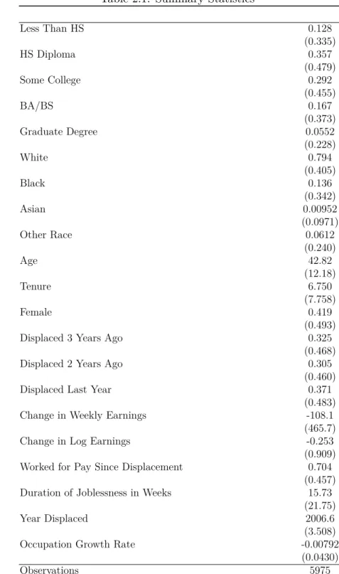
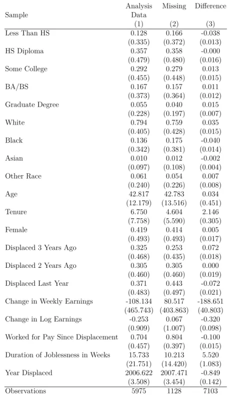
workers who have been displaced from a full-time job. The descriptive statistics for the main analysis sample are reported in Table 2.1.
Displaced workers come from all education categories and races. The average age in the sample is 42.82 years, with 6.75 years of firm tenure. The sample is 41.9 percent female. The mean weekly earnings loss after displacement was $108.1 or 25.3 percent for workers who had been re-employed. This is in the range of previous research on displaced workers and is consistent with the unusually poor labor market conditions following the Great Recession. 70.4 percent of workers worked for pay since displacement.
Additionally, I exclude workers who do not report key variables including pre-displacement occupation, year displaced, full-time status at pre-displacement job and whether the worker moved after displacement.4 The first two variables are necessary to create the
occupation growth rate, which is the focus of my analysis, and the other two variables are key sample selection criteria.5 This is not a trivial restriction: 15.9 percent of
the respondents do not respond to these questions. In Table 2.2, I report tests for differences in observable characteristics between individuals reporting and not reporting pre-displacement occupations. Those reporting, as described, are more educated and have longer pre-displacement tenures.
3I show my results are very similar when including all workers - both those who have moved and
those who have not moved in the Online Appendix.
4Very few survey respondents seem to be selectively responding to certain questions. Instead, the
respondents appear to stop answering questions altogether.
5Occupation growth rates can also not be calculated for workers with sufficiently vague occupations
– if an engineer is not one of the 17 types of engineers listed in the Standard Occupation Classification, he/she falls into the “Engineers, All Other” category, for which the data necessary for a growth rate does not exist. These workers are also excluded from the analysis.
For confidentiality reasons, the DWS does not report finer geography than state for some non-trivial fraction of the sample (approximately 30 percent). As such, state is the geographic labor market used for the analysis.
2.2.2
Occupation-Industry Composition from the Occupational
Employment Statistics
To estimate the effect of the occupation growth rate, I need an annual measure at the state or local level. The American Community Survey (ACS) and other commonly used micro-data cannot be used to calculate a growth rate for most detailed occupations at the state level, since their sample size is inadequate to calculate reliable growth rates for many smaller occupations. Ideally, I would create occupation growth rates using an administrative dataset where employers reported employment levels by occupation annually.
Unfortunately, such dataset does not exist in the United States. The alternative data source for occupation level data is the Occupational Employment Statistics (OES). The OES is a large employer survey conducted by the Bureau of Labor Statistics (BLS) that collects detailed information on employment by occupation, covering 1.2 million establishments and 57 percent of employment in the United States. With a much larger sample size, it is designed to produce detailed estimates of occupation level employment and wages, though these estimates are not suitable for the study of short- term changes. The survey design selected by the BLS divides the establishments surveyed for each set of estimates into panels spread across three years of data. That is, the samples for two adjacent years are not independently drawn, and therefore cannot be used to create an annual growth rate.6 The OES estimates reported by the BLS for a given year are moving
6For example, even a very large private employer will be surveyed every three years. This can make
averages based on three years of survey data.
Even if adjacent years of data were independently drawn, estimates of a single year have greater sampling error, which may be problematic when studying detailed occupations. In fact, Abraham and Spletzer (2009) use the confidential microdata at the detailed occupation level to assess the suitability of the OES for studying the effects of offshoring. They conclude that “employment time series for detailed occupations that are created from single-year micro data are likely to be highly volatile... Increases in the size of the OES sample would be needed to reduce the variance of annual employment estimates” (p. 11).
Because of these limitations, the lack of independence across adjacent years in the sample, and the sampling error associated with a single year’s estimates, the OES cannot be used by itself to produce a state-level occupation growth rate.
The OES also produces estimates of occupation by industry employment at the national level for all years. I use the estimate of occupation by industry employment in 2002 and 2003 to construct an alternative occupation growth rate, along with the industry employment numbers discussed in the next subsection.7 The OES also produces
research estimates of occupation by industry employment at the state level for 2012-2014, which I will use for robustness checks.
2.2.3
Industry Growth Rates from the Quarterly Census of
Employment and Wages
The Quarterly Census of Employment and Wages (QCEW) is a tabulation of employment of all establishments that report to the Unemployment Insurance programs in the United
the local level.
7The use of weights at the beginning is accordance with common practice. However, the results are
States. This employment covers 97% of all wage and salary civilian employment in the U.S. Because every establishment is assigned to an industry, these data are reported at the industry level. I use the annual version of this dataset as the DWS respondents only report their year of displacement. Annual state-level industry employment is used in tandem with the occupation by industry employment composition to construct an estimate of changes in occupational employment. Annual state-level industry employment is also used independently to create a measure of industry growth rate. Occupation data is not available in the QCEW.
2.3
Empirical Approach
My goal is to estimate the effect of the state-level growth rate of a displaced workers’ pre-displacement occupation on his or her labor market outcomes. However, as described earlier, a key challenge is that the OES occupation counts for a single year are estimated using the prior three years of data. Consequentially, major issues – lack of independence across adjacent years, and sampling error associated with a single year’s estimates – impede the estimation of an unbiased coefficient.
To overcome these obstacles, I predict occupation growth from the higher quality data that are available for industry growth. In contrast to occupation level employment, industry level employment is well-measured on a yearly basis. This is because a firm’s product or service determines its industry and this information is easily aggregated using administrative data from unemployment insurance records. Occupations are distributed in different proportions across industries because the composition of labor inputs varies across the production of different goods and services.
If the relevant occupation conditions are at the state level, then the occupation growth rate can be predicted using a state’s industry employment composition, the state-level
occupation-industry distribution, and the growth rate of the industries within the state. In the following subsection, I explain the construction of this state level occupation growth rate measure.
Before continuing, it is important to discuss the level of occupation involved in this analysis. My measure of state-level occupation growth rates in this paper is at the most detailed level available in the Displaced Worker Survey, the Census occupation code. This classification, which comprises 324 Census occupation categories in the estimation sample, is more detailed than the Standard Occupation Classification (SOC) minor group (88 categories) or major group (10 categories). It is also much more detailed than the measure used in existing estimates of the occupation growth rate effects on displaced workers’ outcomes (Carrington, 1993). I use these most detailed codes because it is not clear that occupations within a minor group would have the same growth rate. To see this, consider for example, Table 2.3, which lists examples of major, minor, broad and detailed SOC occupation categories, and Census occupation categories. Using one occupation growth rate for the minor group would assume that the growth rate of word processors and typists (43-9022) is the same as the growth rate of insurance claims and policy processing clerks (43-9031). My approach has the advantage of not imposing this assumption and allowing workers in different Census occupation categories to have different growth rates.
2.3.1
Construction of the State Occupation Growth Rate Measure
To proceed, I create an estimate of the occupation growth rate that does not use the OES as time series data. My decomposition is based on the fact that a given occupation’s employment in a state is the sum of the occupation’s employment in each of the state’s industries.
More concretely, occupation o’s employment in state s at year t, Es,o,t, will be the
sum of state employment in each industry j in that year, Es,j,t, times the fraction of
industry employment in that state and year that belongs to that occupation, αs,o,j,t.
Es,o,t =
X
j
αs,o,j,tEs,j,t (2.1)
Because we are interested in growth rates, we can describe the change in occupational employment in state s and year t as
∆Es,o,t= X j αs,o,j,tEs,j,t− X j αs,o,j,t−1Es,j,t−1 (2.2)
Unfortunately, equation 2.2 suffers from the limitations inherent using OES data for time series analysis, as both αs,o,j,t and αs,o,j,t−1 come from adjacent years of the OES.
For the reasons discussed earlier, this implies that the same employment data is used to determine these two estimates, and these estimates are not independent. However, assuming αs,o,j,t =αs,o,j,t−1∀t, i.e. the share of occupationo in industry j in state s does
not change over time, avoids this issue. This would be true if the production function of various goods and services and the costs of various types of labor are not changing over the sample period. Furthermore, this statement has empirical support – the correlation between national estimates of αo,j,2002 and αo,j,2013, the first and last year, is 0.9 in my
sample. I use a fixed weight from the beginning of the sample to measure α, which I will refer to as αs,o,j,beginning.8
8The first year in which the North American Industry Classification (NAICS) is used in the OES
data is 2002. I use a mean of 2002 and 2003 for the weight, although results are quite similar using only 2002, or some mean of years from the middle of the sample, say 2006-2008.
Then, \ ∆Es,o,t = X j (Es,j,t−Es,j,t−1)αs,o,j,beginning (2.3)
However, I’m interested in a growth rate, as opposed to a pure change in employment. A traditional growth rate measure would use adjacent years of occupation data, treating them as independent. However, recall that the adjacent years of occupation data are not actually independent. To avoid this problem, I use a fixed employment level at the beginning of the data period as the denominator for occupation o’s growth rate in state
s. \ ∆Es,o,t Es,o,beginning = 1 Es,o,beginning X j (Es,j,t−Es,j,t−1)αs,o,j,beginning (2.4) =X j Es,j,beginning Es,o,beginning Es,j,t−Es,j,t−1 Es,j,beginning αs,o,j,beginning (2.5)
The state-level estimates are a function of two potentially noisy measures. It is possible to create variants of this occupation growth rate measure to decrease noise associated with certain state-level estimates. There are two reasons why state level estimates may be substantially noisier than national level estimates: noise in the industry growth rate and noise in the occupation-industry composition.
The 4 digit NAICS industry growth rate at the state level is fairly noisy. Over 14% of the state-industry-year cells have zero employees, and around 20% have fewer than 100 workers. Because of this characteristic, the state-level industry growth rate is highly variable for small industries and small states. Additionally, the displaced workers in my DWS sample may be directly affected by firms closing in their industries, heading to an endogeneity concern. To deal with these problems, researchers including
Autor and Duggan (2003a) have used national-level industry changes in employment, excluding the focal state’s industry employment, which can be denoted by E−s,j,t. This
method, in the spirit of Bartik (1991), has two major advantages: first, it is not reliant on a single state’s noisy industry employment, and second, it decreases the chance of a mechanical correlation between the displaced worker’s job loss and the relevant employment conditions.
State-level occupation-industry composition suffers from a more significant limitation. Namely, the data only exists starting in 2012, and has been published as “research estimates.” This designation implies a higher variability due to smaller samples. Additionally, these estimates are limited to state-occupation-industry cells with sufficient employment to disclose an estimate. As fewer estimates are withheld as employment numbers are aggregated to the national level, national estimates are available for far more occupation-industry cells and for every year in the sample.
Motivated by these concerns, my preferred estimate of the occupation growth rate uses national estimates of both the industry growth rate and occupation by industry composition: πs,o,t= \ ∆Es,o,t Es,o,beginning =X j Es,j,beginning Es,o,beginning αo,j,beginning E−s,j,t−E−s,j,t−1 E−s,j,beginning (2.6)
For clarity, the three components of the measure can be labeled as follows:
πs,o,t= \ ∆Es,o,t Es,o,beginning =X j γs,o,j,beginning | {z } State-specific weight αo,j,beginning | {z } Fraction of occo in indj E−s,j,t−E−s,j,t−1 E−s,j,beginning | {z }
Growth rate of indj
nationally
to “occupation growth rate” as my main regressor of interest for the remainder of the paper.
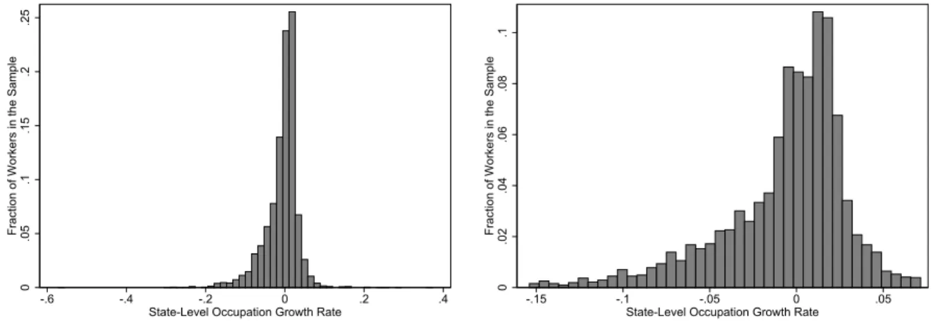
Figure 2.1(a) plots the distribution of occupation growth rates amongst the displaced workers in the sample. The mean worker-weighted occupation growth rate is -0.008 and the standard deviation is .04. Because this figure is less informative because of a small number of large (in absolute value) occupation growth rates at the tail, Figure 2.1(b) plots the distribution excluding the occupation growth rates above the 99th percentile and below the 1st percentile. The figures also show that the distribution is left-skewed.
For comparison, Figure 2.1(c) and (d) plot the distribution of industry growth rates, constructed analogously and discussed in greater detail below in Section 2.3.3. The mean industry growth rate is -0.01, and the standard deviation is 0.05 (a little larger than the standard deviation of the occupation growth rate at 0.05).
2.3.2
Estimation of the Impact of Occupation Growth Rates
I estimate the impact of the occupation growth rate on a displaced worker’s labor market outcomes as follows:
Yi,s,o,t=βπs,o,t+δXi,s,o,t+λs+λt+εi,s,o,t (2.7)
where πs,o,t is the occupation growth rate, defined above. Each displaced worker is
assigned an occupation growth rate based on their state of residence, occupation at displacement, and year of displacement. Xi,s,o,t is a vector of individual characteristics
including sex, race, education, years since displacement, indicators for different age categories, and a quadratic of tenure at the pre-displacement job. λs and λt are state
of residence and year of displacement fixed effects. The primary outcomes of interest,
duration of joblessness, and the change in log earnings. The regressions are weighted by the Displaced Worker Supplement Weights,9 and standard errors are clustered at the
state level. This regression specification compares two observationally identical displaced workers who have been displaced in the same state and same year from occupations growing at different rates.
The identifying assumption in equation (2.7) is that unobservable characteristics of displaced workers are uncorrelated with their occupation growth rate, conditional on observable individual characteristics, state, and year of displacement. This specification directly addresses the challenge of state workforce agencies, who are interested in targeting services to workers and need to decide between workers displaced in a state at similar times.
A potential disadvantage of the specification in equation (2.7) is that workers who select into different occupations may have different unobservable characteristics that affect labor market outcomes, which might be correlated with the occupation growth rate. This might be true, for example, if the most able workers recognize their occupation is shrinking, or vulnerable to shrinking, and change into more stable occupations. To allay concerns about differences in unobservable characteristics across displaced workers in different occupations, I also present estimates that add SOC minor group (3 digit) occupation fixed effects. This specification is as follows:
Yi,s,o,t =βπs,o,t+δXi,s,o,t+λs+λt+λo+εi,s,o,t (2.8)
These fixed effects control for the situation in which certain occupation categories have longer durations of joblessness or lower post-displacement earnings, independent of the occupation growth rate. In this specification, the variation is coming from differences
within occupations, controlling for state and year fixed effects. The identifying assumption is that unobservable characteristics of the worker that affect their durations of joblessness and earnings losses are uncorrelated with their occupation growth rate, conditional on observable individual characteristics, pre-displacement occupation, state, and year of displacement. Of course, while alleviating concerns about bias, equation (2.8) relies on considerably less identifying variation, so it has a cost in terms of statistical power.
As the focus of this paper is displaced workers, I will discuss the magnitude of the effects for a one percentage point decrease in the occupation growth rate.
2.3.3
Comparison with Industry Growth Rate
Previous literature, including Carrington (1993), Kandilov (2010), and Crinò (2010), has found a significant effect of pre-displacement industry decline on displaced workers’ labor market outcomes. However, there are few estimates of the relative impact of occupation growth compared to industry growth in the displaced workers’ literature. Additionally, more state workforce agencies use historical data on changes in industry employment (59%) compared to historical data on changes in occupation employment (25%) in their prediction models (Dickinson et al., 1997).
To compare the impact of industry growth versus occupation growth on displaced workers’ labor market outcomes, I run the following two regressions:
Yi,s,o,t=γπs,j,t+δXi,s,o,t+λs+λt+εi,s,o,t (2.9)
Yi,s,o,t=γπs,j,t+βπs,o,t+δXi,s,o,t+λs+λt+εi,s,o,t (2.10)
where the first equation replaces the occupation growth rate with the state-level industry growth rate. The industry growth rate is analogously predicted from national industry
growth.10 This measure is constructed using the same approach as the occupation growth
rate and therefore has the same advantages: it is not reliant on a single state’s noisy industry employment, and it removes any chance of a mechanical correlation between the displaced worker’s job loss and the relevant employment conditions.
Equation 2.10 adds the occupation growth rate back in. In this equation, the coefficient on occupation growth rate will be the impact of occupation growth holding industry growth constant. Similarly, the coefficient on industry growth rate will be the impact of industry growth holding occupation growth constant.
The labor market outcomes discussed in this context are the log duration of joblessness and change in log earnings. Industry growth is at the three digit NAICS level.
2.4
Results
2.4.1
Variation in the Occupation Growth Rate
Recent research on Bartik instruments by Goldsmith-Pinkham et al. (2018) finds that a number of empirical applications rely heavily on a few industries for identifying variation. In my dataset, this is not the case. The variation in the occupation growth rate in my data is calculated from 291 NAICS 4 digit industries. Figure 2.2 displays a histogram of the number of industries used to derive each occupation growth rate. The figure highlights a key descriptive statistic of the paper: most displaced workers’ occupations exist in a wide number of industries. The mean (median) worker in the sample has an occupation growth rate that is a function of 125 (124) industries. In the extreme, if each occupation is represented in one industry, the occupation growth rate is exactly equal to the industry growth rate. The figure provides one piece of evidence that
10More formally,π
s,j,t=
E−s,j,t−E−s,j,t−1
suggests the occupation and industry growth rate may differ in meaningful ways.
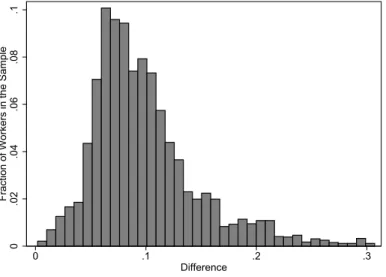
The occupation growth rate also varies substantially over this time period (2001 -2013). Figure 2.3 compares the minimum and maximum occupation growth rates for state-occupation combinations represented in my displaced workers’ sample (i.e. the within-state and occupation across time variation I exploit). The mean difference between the minimum and maximum growth rate is 0.10 and the standard deviation is 0.07.
A second potential problem is that these industries may have characteristics that are correlated with observables, which may suggest potential unobserved confounders. In my context, these are not concerns for the following reasons: First, the fact that different occupations are concentrated in different industries and to different extents is a characteristic of the labor market and an important empirical fact. Second, if a few industries in an occupation are driving occupation growth, occupation growth and industry growth would be highly correlated. The resulting coefficients and standard errors from the regression model would take into account the correlation between the growth rates through the covariance terms in the standard errors. This empirical finding would have an implication for the relative importance of occupation and industry specific human capital – namely, that because of the structure of the labor market, it is difficult to separately identify the effects of occupation and industry specific human capital, and the distinction between the two may be unnecessary.
Because my context is not an instrumental variables context, I cannot measure the sensitivity-to-misspecification elasticity as recommended in the Goldsmith-Pinkham et al. (2018). Finally, in the Robustness section, I show that the estimates are similar when excluding one industry at a time.
2.4.2
The Effect of the Occupation Growth Rate
Table 2.4 shows the effect of the pre-displacement occupation growth rate on the probability of working for pay after displacement, controlling for elapsed time between displacement and the survey date. As the DWS only asks calendar year of displacement, this is only a rough control for elapsed time.11 Working for pay is assumed for workers
currently employed, and asked of individuals who are both unemployed and not in the labor force. Approximately 71 percent of the sample had worked for pay by the time they were surveyed. In Column (1), the specification with state and year of displacement fixed effects, the occupation growth rate does not have a statistically significant, or economically significant, relationship with working for pay after displacement. The biggest determinant of working since displacement is the time elapsed since displacement – workers who were displaced three (two) years ago are approximately 27 (9) percentage points more likely to have worked for pay after displacement, respectively, compared to workers displaced one year ago. The other coefficients in this regression follow expected patterns – older workers are less likely to work after displacement, more educated workers are more likely to work after displacement. In Column (2), the specification adding minor group occupation fixed effects, the occupation growth rate continues to have an insignificant relationship with working for pay after displacement.
The next outcome is log duration of joblessness. Duration of joblessness is defined as the number of weeks that went by between displacement and when the respondent started working again. This is self-reported by all displaced workers who have worked for pay at some time since displacement.12 For other workers, those who have not worked
for pay since displacement, the DWS unfortunately does not ask duration of joblessness.
11Workers are asked which calendar year they were displaced in January. In all regressions, I include
indicators for two calendar years ago and three calendar years ago, with the omitted category being one calendar year ago.
Because the DWS only asks year of displacement, any statements about jobless durations of workers who are not re-employed are highly imprecise.Thus I omit these workers from my main estimates, working with the sample of self-reported completed durations only.13
Approximately 70 percent of workers have worked for pay after displacement, and as discussed earlier, ever working for pay after displacement is largely a function of time elapsed since displacement. In the Robustness section, I report the results from censored duration regressions that include non-re-employed workers under various assumptions for calculating their incomplete durations.
Table 2.5 Column (1) shows that a one percentage point decrease in the growth rate of a worker’s occupation in the state and year of displacement is associated with a 4.5 percent increase in the duration of joblessness conditional on having been re-employed after displacement. The estimate is similar with minor group occupation fixed effects in Column (2) – a one percentage point decrease is associated with a 3.9 percent increase in the duration of joblessness. This translates into a one standard deviation decrease (approximately four percentage points) is associated with a 16.1 percent increase in the duration of joblessness conditional on having been re-employed after displacement.
Previous literature by Poletaev and Robinson (2008) and Kambourov and Manovskii (2009) has focused extensively on the correlation between occupation change and displaced workers’ earnings and employment outcomes. But under what conditions do displaced workers change occupations? Table 2.6 analyzes the effect of the occupation growth rate on the probability of an occupation change for workers who are currently employed. The majority of workers in the sample (64 percent) change occupations after displacement. Linear probability models with occupation change as the dependent variable are displayed in Column (1), and show that a one percentage point decrease in the occupation growth
13As in most censored regression contexts, I expect the exclusion of these incomplete durations
(which will be longer, on average) to attenuate my estimates of occupation growth rates on duration of joblessness. Indeed, this is what I find.
rate is associated with a 0.95 percentage point increase in the probability of an occupation change. Column (2) adds minor group occupation fixed effects, which decrease the magnitude of the point estimate but the new estimate is not statistically different. It appears that workers change occupations because their occupations are shrinking – a one standard deviation lower occupation growth rate is associated with a 3.7 to 4.1 percentage point (5.7-6.4 percent) increase in the probability of changing occupations. This is a large effect of temporary conditions in a worker’s pre-displacement occupation.
Table 2.7 looks at the change in log earnings between pre- and post-displacement jobs, conditional on re-employment. Earnings changes are related to the worker’s occupation growth rate: a one percentage point decrease in the occupation growth rate is associated with a 1.5 percent decrease in post-displacement earnings. This effect is similar when adding minor goup occupation fixed effects – a one percentage point decrease in the occupation growth rate is associated with a 2.2 percent decrease in post-displacement earnings. The standard deviation of the occupation growth rate amongst this sample is 0.042, suggesting that a worker who is displaced in conditions one standard deviation below the mean suffers, all else equal, a 9.2 percent larger earnings loss than a worker displaced in conditions at the mean.
2.4.3
Comparison with Industry Growth
With a clear understanding of the negative impact of the occupation growth rate on displaced workers’ labor market outcomes, I now turn to understanding its role relative to the industry growth rate. Before presenting regression results on these relationships, I begin by showing descriptive evidence. In Figure 2.4, the occupation and industry growth rate are split into five categories: shrinking substantially, shrinking, neutral, growing slightly, and growing substantially. The mean and 95% confidence interval is
displayed for workers in each of these categories. In Figure 2.4(a), the range spanned by the means and confidence intervals of the occupation growth rate is larger than the range spanned by the means and confidence intervals of the industry growth rate. A similar story appears in Figure 2.4(b), the equivalent figure for change in log earnings. Workers displaced when their occupation is shrinking substantially have larger earnings losses than when their occupation is growing substantially (p = 0.0757). This is not true of workers displaced when their industry is shrinking substantially compared to workers displaced when their industry is growing substantially (p = 0.3938). However, these results can be driven only by differences amongst workers in these samples and/or state and year of displacement characteristics. Table 2.8 more formally tests the relative effects of occupation and industry growth rates.
Table 2.8 Panel A compares the impact of occupation versus industry growth on the duration of joblessness. Column (1) shows that a one percentage point decrease in the occupation growth rate is associated with a 4.5 percent longer duration of joblessness. Column (2) shows that a decrease in the industry growth rate has a smaller effect on duration of joblessness, but still lengthens it – a one percentage point decrease in the industry growth rate is associated with a 2.1 percent increase in the duration of joblessness. These coefficients, in Columns (1) and (2), are also statistically different. Column (3) includes both the occupation and industry growth rates in the same regression. While the magnitude of the occupation growth rate shrinks slightly, it is still statistically and economically significant. The industry growth rate coefficient is also smaller, and now not statistically significant. The relative magnitudes here are important – the point estimate on the occupation growth rate is ten times the size of the point estimate on the industry growth rate. The test of equality between the two coefficients in the regression shows that we can reject the null hypothesis that these growth rates are the same at the 1% level.
Columns (4) - (6) add minor group occupation fixed effects to the specifications in Columns (1) - (3). These fixed effects do not significantly change the magnitude of the estimates. A one percentage point decrease in the occupation growth rate is associated with a 3.9 percent longer duration of joblessness. On the other hand, the effect of a one percentage point decrease in the industry growth rate is a statistically insignificant 1.2 percent. Column (6) shows the “horse race” regression specified in Equation 2.8. Again, the effect of the occupation growth rate is much larger than the effect of industry growth rate. As in Column (3), the industry growth rate has a quite small impact on duration of joblessness. It is valuable to remember that the occupation growth rate is constructed using industry growth rates. As such, it should not be surprising that the correlation between the occupation growth rate and the industry growth rate is 0.70 in this sample. Despite this fact, the estimated occupation growth rate effect is statistically different in both comparisons in Table 2.8.
Table 2.8 Panel B compares the impact of industry and occupation growth on the displaced workers’ change in log earnings. A one percentage point decrease in the occupation growth rate is associated with a 1.5 percent decrease in earnings. A one percentage point decrease in the industry growth rate is associated with a 0.9 percent decrease in weekly earnings. The coefficient on the occupation growth rate is larger, though not significantly larger, than the coefficient on industry growth rate. When the occupation growth rate and industry growth rate are in the same regression, as in column (3), neither effect is statistically significant although we can reject the null hypothesis that they are jointly equal to zero (p= 0.0037). A similar story can be told with occupation fixed effects in columns (4)-(6).
2.5
Robustness
This section assesses the robustness of these results to a variety of potential concerns. The first concern is whether the occupation growth rate used is truly a measure of temporary conditions at the time of displacement, or if it reflects something systematic about the occupational labor market. If the effect is truly the effect of displacement during poor labor market conditions, then it should be largest for the contemporaneous occupation growth rate, and not the occupation growth rate in years prior to displacement. Table 2.9 compares the specification based on the contemporaneous occupation growth rate with the occupation growth rate last year, the occupation growth rate two years ago, and the mean occupation growth rate in the three years leading up to the displacement (the contemporaneous year, the year prior and two years prior). To make comparisons across these four specifications, the sample is limited to workers who have all four measures, decreasing the sample size by excluding workers displaced in 2001 and 2002. The contemporaneous growth rate, in Table 2.9 Panel A Columns (1) and (5), has the largest effect on the worker’s duration of joblessness, followed by the mean growth rate. Panel B, which changes the focus to change in log earnings, provides more support for the contemporaneous growth rate. Here, the contemporaneous growth rate is the only statistically significant estimate. The mean growth rate, in this case, even has the ‘wrong’ sign (Column 8).
To ensure that this effect is truly the effect of temporary labor market conditions at displacement, I run a placebo test, comparing the effect of the contemporaneous occupation growth rate with the effect of the occupation growth rate four years after displacement on the worker’s duration of joblessness. The sample is limited to workers for whom both contemporaneous and four year later occupation growth rates are available, and therefore, workers displaced after 2010 are excluded. By four years after the reported
calendar year of displacement, the vast majority of displaced workers have been re-employed, and therefore the occupation growth rate should have little effect on the worker’s duration of joblessness. In Table 2.11, the occupation growth rate four years after displacement has a significant effect on duration of joblessness in the absence of controls for occupation. This is surprising as the occupation growth rate four years later is negatively correlated with the contemporaneous occupation growth rate (ρ =
−0.2385). In Column (4), which adds minor group occupation fixed effects, the estimate of the occupation growth rate four years later becomes much smaller and is statistically insignificant.14
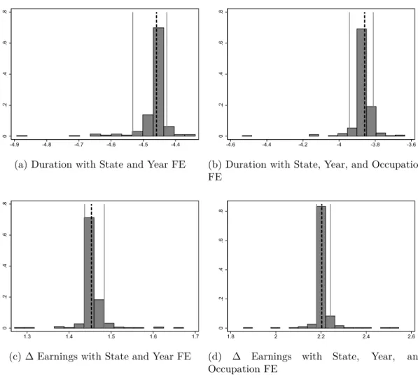
As previously discussed, recent literature on shift-share approaches by Goldsmith-Pinkham et al. (2018) suggests that many empirical applications rely on a few industries for identifying variation. If one industry is driving the results, it also may be true that this industry’s growth or decline is not exogenous to the worker and/or is correlated with the unobservable characteristics related to the worker’s labor market conditions. To show that the occupation growth rate is not being driven by a singular industry’s employment changes, I construct the occupation growth rate leaving out one industry at a time, then run the main regressions with these new “leave-one-out” growth rates. The result is 291 estimates of the occupation growth rate’s effect on each outcome. Figure 2.5 displays histograms of the estimates for the four primary outcomes: log duration of joblessness
14While it seems plausible to expect no effects of the growth rate of a worker’s pre-displacement
occupation four years after displacement on the length of the worker’s first post-displacement jobless spell (an outcome that is most likely determined by that time), a similar null effect does not seem likely on the worker’s earnings at the DWS survey date, which can be up to three years after displacement. Employment growth (estimated by the growth of occupation o between t+ 3 and t+ 4) in the pre-displacement occupation should still be correlated with the worker’s outside options, since he or she has skills related to that occupation, for reasons explored by Beaudry et al. (2012) and Tschopp (2017). For these reasons, Table 2.11 type regressions do not constitute a valid placebo test when earnings are the outcome of interest. Interestingly, while the standard errors are large, four-year-later occupation growth rates in those regressions have consistently positive coefficients, regardless of whether the worker has switched occupations. I interpret this as suggestive evidence of search and bargaining effects in local labor markets.
and change in log earnings, with and without occupation fixed effects. The original estimate of the occupation growth rate (with all industries) is denoted by a dashed line. The 95 percent confidence interval of “leave-one-out” estimates is denoted by solid lines. From these figures, it is clear that the occupation growth rate is insensitive to any single industry’s employment.
The occupation growth rate, however, is constructed such that is mechanically correlated with the industry growth rate. While the above robustness check suggests that this mechanical correlation is unlikely to drive the results, it may impede the interpretation of the coefficients as representing independent factors. To address this concern, I develop an alternative occupation growth rate measure, defined as
πs,o,−j,t = \ ∆Es,o,t Es,o,beginning = X j!=j0 γs,o,j,beginning | {z } State-specific weight αo,j,beginning | {z } Fraction of occo in indj E−s,j,t−E−s,j,t−1 E−s,j,beginning | {z }
Growth rate of indj
nationally
(2.11)
where the weighted average intentionally excludes industryj, the industry that displaced worker in the sample was displaced from. To put this more concretely, the millwright who was displaced from a transportation equipment manufacturing plant has an occupation growth rate that is a function of all the industries in his state, excluding transportation equipment manufacturing. The estimation equation, therefore, is
Yi,s,o,t=γπs,j,t+βπs,o,−j,t+δXi,s,o,t+λs+λt+εi,s,o,t (2.12)
The coefficient on πs,o,−j,t is expected to be smaller in magnitude than the preferred
specification, as this new measure excludes the growth of the industry that that displaced worker is most likely to find work in.
The coefficients on the newly constructed occupation growth rate are similar to the prior specifications, e.g. one percentage point decrease in the occupation growth rate is associated with a 5.1 - 5.6 percent increase in duration of joblessness. The test for equality row suggests that despite this handicap on the occupation growth rate, it continues to outperform the industry growth rate in its relevance for duration of joblessness. The results for change in log earnings are similar, but without much precision. Unsurprisingly, the standard errors on the estimates are larger, and the new correlation between occupation and industry growth rates is smaller (ρ= 0.515).
Another concern may be the sensitivity to the way the occupation growth rate is specified. To address this concern, I vary the method by which I estimate the occupation growth rate. Table 2.12 shows the effect of the occupation growth rate measured in four different ways on log duration of joblessness and change in log earnings. As discussed in section 4.1, my preferred measure of the occupation growth rate uses Equation 2.6, displayed in Columns (1) and (2) of Table 2.12. The three components of this measure are the state-specific weight and national estimates of the industry growth rate and national estimates of occupation by industry composition. To show robustness to different measures, I replace the national occupation by industry composition term with a state-specific occupation by industry composition term. This comes from the OES research estimates of state-level occupation by industry employment, which started in 2012. In other words, I replace αo,j,beginning with αs,o,j,2012 in Equation 2.6. This estimate is
displayed in Column (3) and (4) in Table 2.12 with and without occupation fixed effects. The estimate is smaller than the corresponding estimates using the national occupation by industry composition term but still statistically significant.
The next measure of occupation growth rate returns to Equation 2.6 and replaces national industry growth with state s’s industry growth. This estimate is displayed in Columns (5) and (6). The estimate is smaller than the estimates from Column
(1) and (2) but still economically meaningful (notably, bigger than the estimates of the industry growth rate from 2.8). Finally, in Columns (7) and (8), the occupation growth rate measure combines the two changes. This estimate is the smallest of the four, but still statistically significant. The pattern is similar when considering changes in weekly earnings, though the results become insignificant when using the own state industry growth rate. The weaker estimates when using state level industry growth may be evidence of greater measurement error in these values.
As the Displaced Workers Survey does not ask duration of joblessness for individuals who have not been re-employed by the CPS survey date, my main results on duration of joblessness did not include those who have not been re-employed. While Table 2.4 shows that the occupation growth rate does not have a significant effect on the probability of working for pay after displacement, a concern may be that my estimated effects of the occupation growth rate are affected by right-censoring of observed durations. This concern is addressed in Table 2.13, which demonstrates robustness of the log duration of joblessness result by including workers who have not been re-employed. The DWS