The Effect of Sample Composition on the
Estimation of Development Patterns
Bankc Staff Working Paper No. 204
-. 'D
-* .
.1
* ., *9 .^.
Public Disclosure Authorized
Public Disclosure Authorized
Public Disclosure Authorized
Public Disclosure Authorized
Public Disclosure Authorized
Public Disclosure Authorized
Public Disclosure Authorized
This paper is for staff use The views expressed are those of the author and not necessarily those of the Bank.
INTERNATIONAL BANK FOR RECONSTRUCTION AND DEVELOPMENT
Staff Working Paper No. 204
THE EFFECT OF SAMPLE COMPOSITION ON THE
ESTIMATION OF DEVELOPMENT PATTERNS
May 1975
This paper describes in detail the methodology utilized in Patterns of Development 1950-1970 by Chenery and Syrquin
(Oxford Press 1975). It is written as a technical annex to that work and specifically addresses the problems of estimation in a large pooled tmes series and cross section data sample. It is recommended that this paper be read in conjunction with Patterns of Development and not separately.
The analysis is based on research done under the World Bank Research Pr-ogram, Project RPO 205 ("Cross-Section Analysis of Development Research Patterns").
Prepared by Moises Syrquin (assisted by Haze7 Elkington)
THE EFFECT OF SAMPLE COMPOSITION ON THE ESTIMATION OF DEVELOPMENT PATTERNS
I
Intercountry comparisons play an essential part in understanding the processes of economic and social development. lo generalize from the experience of a single country or region we must compare it in some way to that of other countries.
The great inr.crease in statistical information since 1950 has
allowed many detailed comparisons focusing on individual characteristics of developing countries such as consumption, saving, industrialization and popuilation growth. However, since these studies apply a variety of
statistical methods to different country samples and time periods their results are not generally comparable.
A recently completed study (Chenery and Syrquin, 1975) provides a comprehensive description of the structural changes that accompany the growth of developing countries by applying a uniform statistical procedure to the estimation of a wide range of development patterns (variations in different aspects of the economic structure in relation to income level and other factors) for a maximum of 101 countries over the period 1950-1970.
To achieve broad coverage of the various features of development, this study concentrated on twenty-seven variables - describing ten basic processes of accumulation, resource allocation, and income distribution r
that are included in the IBRD economic and social data bank.
The large size of tthe sample and its broad composition made possible more representative cross-country studies. The experience of countries at
low income levels could now be tako;n into account. In earlier studies this was not feasiblco as the basi-c data were not available and in many cases the countries had not yet come into existence.
Comprehensiveness of the sample is desirable to make the results more meaningful. Yet iu also b:rings in problems of comparability and interpretation,,as in oux c-se where the noise element in the data of low income countries is probably quite large and where the country composition of the sample is not uniform over time.
The purpose of this paper is to examine the effects of sample
composition on the estimation of development patterns. To this end we chose one of the allocation prceesse;i wi-th a long history of cross-country
studies., namely the changii-, structure; of production (value-added). Two main
aspects will be analyzed: a) The addition of countries over time may produce temporal shifts if the new countralia0es development patterns do not coincide with those of the original C:'twiea We therefore compare the results
obtained when using maximal saxnples with those obtained for a reduced compatible
sample whose composition does not vary over time. b) In some cases the
specific characteristics of a few countries unduly dominate the results for
any given year0 While it is `½.*'rue that by leaving out extreme observations
the statistical fit could always be improved3 the gain in accuracy would often be an illusory one. In Chenery and Syrquin., (1975) such a practice was
avoided. It is nevertheless of interest to identify the outliers in order to detenmine whet-her their deviance is due to errors of specification (factors
omitted from the anialysi.s, midsspee.ified functional form, etc.), or to
transient pheinomena which only- a dynamic (disequilibrium) model could incorporate.
-3-of changes in the sectoral structure -3-of production and resource use, the
econometric procedure employed here and in Chenery and Syrquin (1975) is described. In part II the results of estimating annual cross-sections for the various samples are compared primarily for the components of commodity output (primary and industrial production). Then in part III the case of the services sector is treated separately.
Past Work on the Patterns of Industrialization
The search for empirical regularities in the sectoral distribution of economic activity goes back at least to Fisher (1939) and Clark (1940)
who observed the progression in the allocation of labor from primary to secondary to tertiary employment. This observation was explained by Clark
largely on thebasis of changes in domestic demand. The subsequent work of Kuznets (1957, 1971), Chenery (1960),and other scholars showed the need for a more comprehensive treatment of both demand and supply factors in seeking
to explain allocation patterns. Chenery (1960) first used econometric
techniques to estimate a set of semi-reduced forms derived from a general equilibrium model.!/ The data input consisted then of one single observation for about 50 countries.
Kuznetst work which also included analysis of the time-series data available then for a score of high-income developed countries, demonstrated the similarities between historical growth patterns and th; intercountry patters of the 19501s?1. Short time series of LDC's appear first in Chenery
and Taylor (1968) where the by then respectable sample (both across countries and over time) allowed refinements in the econometric procedures and a first attempt to identify alternative-patterns of development for different country
-4
groups. By combining cross-section ith time series data_,questions left unanswered in previous studies began to be analyzed, - notably those concerned with the temporal stability of the observed intercountry patterns and the nature of the time trends. These questions are extensively discussed in
Chenery and Syvquin (1975) and are the main subject of part II below. Econometric Procedure
The basic hypothesis underlying the estimation is that development processes occur with sufficient uniformity among countries to produce a
consistent pattem of change in the structure of production as the level of per capita income rises.
To test and quantify this hypothesis, equation 1 (below) and variants of it were estimated for the four components into which we disaggregated the total gross domestic product
(GDP)-Sector Value added in production SIC 3
Primary (Vp) Agriculture and Mining 0 + 1
Industry (Vm) Manufacturing and Construction 2 - 4
Utilities (Vu) Utilities 5 + 7
Services (Vs) Services 6+8-81
The total sample consisted of the 89 countries with at least five annual observations during the period 1950-1970, excluding most of the
communist economies and countries where the population in 1960 was below one million. This brought t,he number of observations for the whole period to 1325. (l) V4 i4( + n
Y
(2 n y)2 y1 n N (ln N)2 +2S. T. +£ FwhereW Vi = dependent variable with i = p, mIn u, So
Y = GNP per capita in 1964 US dollars.
T = time dummies for pooled regressions (j=1,2,3,4)
F = net resource inflow (imports minus exports of goods and non
factor services ) as a share of total GDP. The rationale for this specification is as follows:
1) The share specification of the dependent variable leads to consistent estimates of each component of production. The adding up criterionV,
where the sum of all shares must total 100 per cent and the partial effects of each exogenous variable must total zero, is satisfied for this semilog function. We make use of this property in the sequel where the results for the utilities share are omitted. i
2) Per capita income (Y) serves as an overall index of deveopment. The quadratic term is added to represent nonlinearities inherent in the analysis, as the shares are bounded by zero and one. Although a logistic type curve would often provide a more satisfactory representation of many devebpment processes, there are rarely sufficient observations over the central income range ($100 to $1000) to moke it a significant improvement over this simpler form.
3) The country's population (N) is introduced as an independent variable to allow for the effects of economies of scale and transport cosb on the patterns of production directly and through its effect on the patterns of trade.
l) The net resource inflow (F) affects directly or indirectly a number of development processes. (For details see Chenery and Syrquin, l975). In our case F may be expected to alter the production structure through its differential impact on the production of tradeable and home goods (mainly services,'
5) The time duamies are added when the various cross sections are pooled,to represent exogenous shifts in the structural relationships over time. Five-year periods were used in measuring T which correspond to 1950-54(T=1)5 1955-59(T=2), 1960-64(T=3). Post 1964 observations form the reference period to which the regressions in the tables refer.
6-.11
The lar-ge sample across countries and over time made possible alternative ways of analyzing the data. To take adcvantage of the large variation across countries cross sections relations were estimated first for each year of the 1950o1969z/ period and then for the period as a whole. This follows the classical procedure for pooling which postulates a general hypothesis (in this case that each year has a different relation) and then successively tests the nested hypothesis of homogeneity of subgroups.y The Samples
As mentioned above,to Esess the impact on the relations of the changing composition in the sample two sets of samples were defined: maximal (full) ones including all the countries with the relevant data fc;L a given year/, arnd a compatible kreduced) sample including the forty-two countries with annual observations on all the relevant variables for the 1950-1964 period. Full
samples range from forty-four countries in 1951 to a maximum of eighty-six in 1964. LDCs appear in the full samples during the 1950s with the very poor countries entering later.
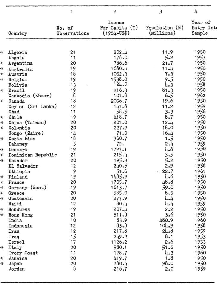
The sample sizes and unweighted average per capita income by year are presented in Table 1. The list of countries and the dates at which each one
entered the samples appear in Table Al in the appendix. For countries in the maximal but not in the compatible sample, the average income per capita in
1955 is about one-half ol the average per capita income in the compatible sample ($334 and $608 respectively). After that it declines through 1962 in spite of the general increase in income in most of the countries, as new and ever poorer countries are added to the sample. Average income for the
-7-TABIJS 1
Number of Countries Included in the Compatible and full Samples by Ya
Full Sample Co npatible Not In CoEpatible
Year n Y n Y n Y 1950
45
524 42 524 3 524L-1951 44 517 42 539 2 55L 1952 46 537 42 5494
411 1953 50 506 42 570 8 170 1954 53 526 42 582 11 312 1955 54 547 42 608 12 334w 1956 56 518 42 623 14 203 1957 55 538 42 639 13 212 1958 60 508 42 641 18 198 1959 66 506 42 661 24 235 1960 75 486 42 690 33 226 1961 77 472 42 713 35 183 1962 78 482 42 735 36 187 1963 82 480 42 758 40 188 1964 86 509 42 805 44 226 1965 85 532 42 829 43 242 1966 85 537 42 851 43 212 1967 81 580 42 873 39 264 1968 73 554 1969 53 422 n Number of countries.Y = Unweighted average per capita incoze for the sample.
l
The three countries with 1950 data but not in the compatible sample are Congo., New Zealand, and Nigeria. For New Zealand we do not have an observation in 1951.complete sample also falls during that period but goes up by almost 25% within the 42 countries in the compatible sample.
Annual Cross Sections
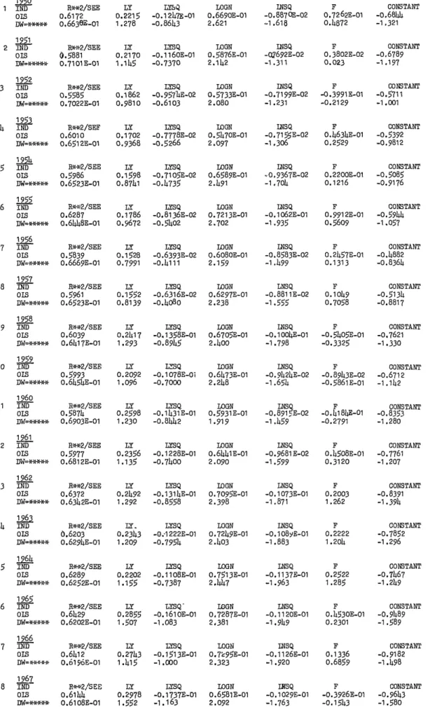
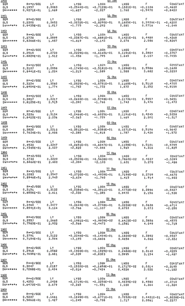
Annual cross sections are estimated for both sets of samples: 20 for the full samples (l950-69) and 18 for the reduced (1950-67). The results for the output shares of primary., industry and services appear on Tables A2
-A7 in the appendix.
The coefficients of the income variables are quite significant in almost all the regressions. In the few cases where they are on the border-line of statistical significance, dropping the nonborder-linear income term results in highly significant income effects. The curvature of the patterns is more pronounced in the full than in the reduced samples, where the limited representation of countries at the lower end of trie income scale makes it harder to detect significant non-linear effects. Of particular interest in this respect is the comparative behavior of the services relations which is analyzed in part III.
The year-by-year coefficients of income reveal a systematic reduction over time in the magnitude of the non-linear tern in the primary and industry regressions for the full but not for the compatible samples. This change implies that over time, the intercountry variation with (the log of) income,
of the shares of commodity production, hits become more linear. This tendency
is absent from the results for the compatible sample which implies that the reduction in the non-linearities can be traced to the production structure of the countries joining the maximal samples over time. For the industrial sector the compatible regressions actually become more non-linear over time probably reflecting the acceleration in the transformation of the medium
9-income countries during the transition and the poor representation of the very low income countries in those samples.
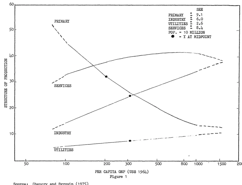
To determine whether any single cross section can be taken as representative or whether the relation has not remained stable over time, cross section patterns were derived from the pooled samples. These are given in Table 2. The implied relation of the structure of production with per capita income for the full sample is plotted in figure 1 for a
typical country of 10 million population and normal capital inflow for each income level. 1l/
The coefficients of the time variables represent the amount by which the re.lation was uniforml higher (if positive) or lower (if negative) in the corresponding period relatively to the post 1965 period. Thus, an upward shift of one percent point each five years would yield the following
coefficients.
T1 = -. 03,. T2= -. 02, and T - 01.
The results are quite similar for both samples. The main differences parallel the ones encountered in the annual cross sections. The reduced sample, for example, shows less curvature for the primary and services shares but
a larger curvature term for industry.
In both sets of cross sectionss statistical tests reject the assumption of homogeneity of the annual regressions. These tests are discussed at length
in the Technical Appendix to Chenery and Syrquin 1975, pp.163-167 and Johnston(1972).
The results of the corresponding F tests are:
SPz
Sector Full Reduced
Primary 19.3 9.5
Industry 21.2 2.1
Degrees of freedom (6,131) (6,744)
Note: For these tests the pooled regressions were estimated without the time variables.
10
-TABLE 2
PRODUCTION PATTERNS FOR THE MAXIMAL AND COMPATIBLE SAMPLES
Constant lnY (lnY)2 lnN (1)2 F T T T SEE No. of
12 3 Os Primary Output Full 2.025 -. 456 .028 -. 030 .004 -. 588 .012 .011 .010 .754 .079 1325 (26.10) (17.23) (12.27) (5.027) (3.131) (20.21) (1.879) (1.863) (1.807) Reduced 1.672 -. 360 .021 .001 -. 0036 -. 496 .020 .014 .006 .713 .063 756 (13.19) (8.761) (6.243) (.229) (2.838) (13.04) (2.811) (1.900) (.905) Industry Output Full -. 547 .158 -. 006 .060 -. 008 .213 .011 .003 -.004 .714 .057 1325 (9.759) (8.260) (3.812) (13.94) (9.405) (10.15) (2.361) (.745) (.938) Reduced -.646 .197 -.010 .o65 -.010 .057 .010 .006 .003 .607 .061 756 (5.245) (4.926) (2.988) (10.53) (7.724) (1.540) (1.464) (.818) (.436) Service Output Full -.473 .291 -.022 -.0O4 .006 .360 -.018 -.011 -.006 .299 .079 1325 (6.113) (11.01) (9.945) (6.758) (5-357) (12.41) (2.682) (1.855) (.969) Reduced .021 .147 -.011 -.078 .015 .431 -.029 -.020 -.011 .301 .067 756 (.155) (3.340) (3.241) (11.37) (11.28) (10.63) (3.702) (2.638) (1.446) t ratios in parentheses
Even though the stability hypothesis was rejected, pooled regressions are still useful. In addition to making use of all the information, they are more suitable to use than any one cross section when interpreted as
averaging the various non-homogeneous cross aections. By adding a set of time dummy variables to the pooled regression, as in Table 2, all variation in
intercepts between time periods is eliminated. The estimated regression is then a weighted average of the various cross section regressions with weights
related to the within-time-period variances of the explanatory variables. The estimates of the tie-dumnmy variables may reflect the independent effect of universal processes such as changes in technology, but in addition they capture time-related problems of specification. To appreciate the size and importance of the temporal variation in the amnual cross sections for both sets of samples and the differences between the two sets, predicted values from each cross section regression were calculated at four benchmark levels of income for a typical country of 10 mil-lion population and foreign capital inflow of two percent. The mean predicted values for the 1950s and 1960s are given in Table 3.
The predicted primary share at low income levels is larger when using the maximal samples but only within the decade of the fifties; in the following years it is almost the same or even lower than the predicted shares from the reduced sample. The reasons have to do with variations in the composition of the sample. There are almost no countries with aery high primary share in the reduced sample. The predietions at the lower income end for this sample are merely extrapolations of the type of curvature encountered at medium and high income levels, while the higher figure for the 1950s in the maximal samples does represent the structure of economies at such a level of income.
PERCENT GDP 60
SEE
PRIMARY +91
PRIMARY IUTILITIES INDUSTRY t 6.02.6
50 SERVICES - 8.4 POP. = 10 MILLION * = Y AT MIDPOINT
ho\
0 -0 E-) u20 -10 INDUSTRY . - 1 UTILITIES 50 100 200 300 500 800 1000 1500 2000PER CAPITA GNP (uS$ 1964) Figure 1
Source: Chen4.rv and Srocuin (1975)
Note. The estimated variation is plotted from $100 to $1000. Average observed values are also
given for countries below $100 and above $1000 per capita income. These are connected by dashed lines to the regression results. Nornal capital inflow for each income level.
- 13 °
Although the countries that were being added to the full samples during the fifties had relatively high primary production shares, they experienced a small fall in the value of the share, only part of which was related to income. Thus, while in the period 1953-1956, the countries not in the compatible sample had an (unweighted) average income and primary share of $255 and .418 respectivel)y, in 1963-1966 the countries outside the compatible
sample (a much larger number by then) had a significantly lower income level ($217) but practically the same primary share (.419).
This downward shift over time is quite stronger at the upper end of the income scale, but it is not adequately represented in the pooled estimates in Table 2. The tine variables there are intended to represent uniform shifts but not trends specific to certain income ranges. For this task separate pooled regressions were estimated for countries classified into
poorer and richer, depending on whether their 1960 per capita income level was below or above $500.U/ The results in Table A8 in the appendix, confirm the
significant time effects for the higher income countries, which imply that after 1965 a typical country in this group would have had an expected primary share in output almost five percentage points lower, compensated by an expected services share of more than five points higher than their predicted average vallues for the 1950-54 period. This is roughly what the figures in Table 3
suggest.
This finding of a differential time trend by level of income, whose exploration lies beyond the scope of this paper,9 could only be inferred from a detailed analysis of the various cross sections, such as attempted here.
The normal variation with income from the annual regressions for the industrial share (in Tables A2 to A7 in the appendix) indicate that the income
TA1 3
Average Predicted Values of Production Shares fromL Yearly Cross Sections
Full Sample Reduced Sample
Per Capita Income Per Capita Income
Period (US$1964) (US$1964)
Production $50 $300 $800 $1,500 $50 $300 $800 $1,500 1950s: Primary 64 27 17 17-13tL 57 28 18 15 Industry 6 27 35 38 9 28 34 38 Utilities 3 7 9 10 5 7 10 10 Services 27 39 39 3 3-3 7L2 29 37 38 37 100 100 100 100 100 100 100 100 1960s: Primary 60 26 14 9 59 27 15 11 Industry 10 25 33 38 4 27 35 39 Utilities 3 8 10 10 3 7 10 10 Services 27 41
143
43
34
39
-40
40
100 100 100 100 100 100 100 100Source: Tables A2 - A7 in the Appendix
L Within the decade there was a systematic trend from the first to the second value.
-
5-pattern tends to rotate in opposite directions for the two sets of samples: "clockwise" for the maximal samples (intercepts increase, income elasticities decrease; predicted values go down at low income levels and up at high income levels), and "counterclockwise" for the compatible sample. These facts can be reconciled by comparing the industrial structure of the poorer countries not in the compatible sample with that of the remaining countries and by
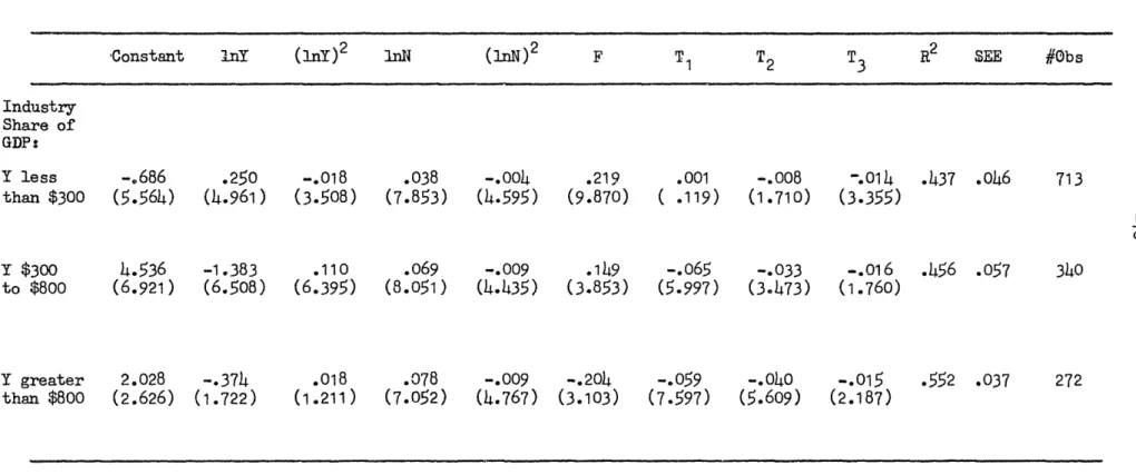
assuming the "true"' within-country pattern to have a logistic type shape. Though the results of the two way income split in Table A8 suggest such a pattern, a better approximation can be obtained by dividing the sample into three income groups. The results of such a split for the industry share
(Table 4) support the logistic hypothesis, primarily through the acceleration of the income-related changes during the medium income transition range.
During the fifties the compatible sample had few observations in the middle region where the process accelerates. Most of the countries were at either end of the income scale. By the sixties, however, many
countries moved into the accelerating stage, and at the same time an exogenous upward shift was observed in all but the low income countries (Table 4). In order to ;ncorporate these changes the annual semilog cross section regressions had to shift counterclockwise. This rotation adequately captureri the position of countries in the transition range, but it yielded unreasonably low predicted values for the low income range with no serious consequences since the
compatible samples are unpopulated at that range.
In the maximal samples, however, there are 44 countries which are included in the observations at one point or another after 1950, 38 of which had in 1965 a per capita income below $250, and in 21 of these it was even
TABLE 4: Industrial Patterns By Income Groups
'Constant TnY (ny) 2 jTI (inN)2 F T1 T2 T3 R2 SEE #Obs
Industry Share of GDP: Y less -.686 .250 -. 018 .038 -.004 .219 .001 -.008 -.014 .437 .046 713 than $300 (5.564) (4.961) (3.508) (7.853) (4.595) (9.870) ( .119) (1.710) (3.355) Y $300 4.536 -1.383 .110 o69 -.009 .149 -.065 -.033 -. 016 .456 .057 340 to $800 (6.921) (6.508) (6.395) (8.051) (4.435) (3.853) (5.997) (3.473) (1.760) Y greater 2.028 -.374 .018 .078 -.009 -.204 -.059 -.040 -. 015 .552 .037 272 than $800 (2.626) (1.722) (1.211) (7.052) (4.767) (3.103) (7.597) (5.609) (2.187) t ratios in parentheses.
-17-the observed 1965 average industrial share was equal to a relatively high .134. In order to incorporate these observations (relative high industrial share at low income levels) into a uniform semilog regression, a typical cross section curve in the 1960's had to shift in a clock-wise direction relative to a typical cross section during the 1950's. This rotation, as seen from the predicted values in Table 3, took place in spite of the accelerating industrialization of the countries in the transition range.
All these elements can be graphically il-lustrated with the aid of Figure 2. Vm logistic -- 1960 full a10/
1960
reduced O countries in 1950 C. X countries in 1960 E- New countries - 1960 lnY Figure 2If we take line A. to represent the estimated relation during the 1950's for both samples, then the progression of countries into the accelerating range shifts the estimated curve for the reduced sample to the line B. But the least squares line will have to shift clockwise to line C in order to incorporate the relatively high share of the new,
low income countries.
The time trends for the industrial share implied by the pooled regressions in Table 2 - an insignificant fall for the reduced sample and a nonmonotonic variation in the maximal sample - are the result of a composition of the sample effect and of differential time shifts by income groups. The early fall in the full but not in the reduced,
results from varying the sample, and the very small upward shift after-wards averages the presence of a significant upward trend in the middle and lhigh income groups. (see Table 4) and its absence in the poorer countries.
The complication which a varying sample composition creates for separating time and income effects can be analyzed in still one more way by trying to eliminate the main source of instability, namely, variation among countries.
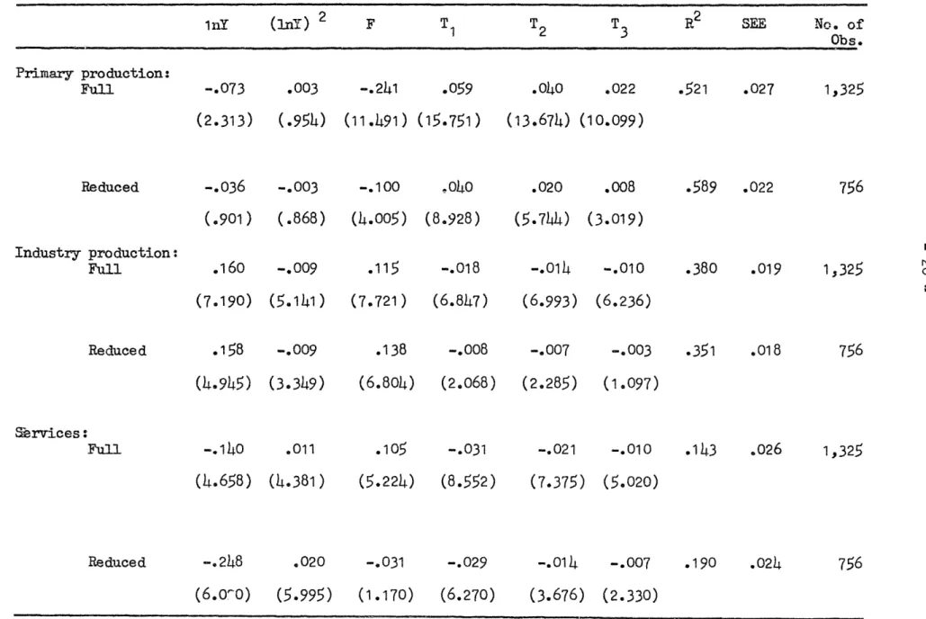
By adding a set of country dummy variables (one for each country) to equation 1 we obtain in fact an average of the time series experience within countries over the 1950-1970 period. 1!4/ Table 5 presents such short run estimates for the structure of production. (Note that the constant term is omitted since we now have a separate intercept for each country). Once the variation between countries has been removed, the composition of the rmple is less important, and time trends become quit%'. significant: downward for the primary share and upward for industry in both samples, but more so in the maximal one. This last result is
what the import-substitution drive which pervaded a large part of the
developing world woul-d .jave led us to expect.
The composition of the sample seems to be an important factor in analyzing cross sections of country data over time in the post
1950
-1
9-period. As the number of yearly observations increases for all countries
and since a large number of new countries is not expected to enter the
sample, this effect will clearly diminish in importance in the future.
III
Although the composition of a sample and its varying coverage over time can affect the uniform regressions, much of the impact of the
changing composition of the sample is adequately reflected in the uniform patterns through the time-shift variables. The case of the services
sector is treated separately here as a unique example of a situation where the specific characteristics of a few countries unduly dominate the results
for any given year. The problem is not so much the result of a changing sample over time as it is one that is present all through the period, although there are signs that over time the exceptional countries are becoming less differentiated in their industrial structure.
The Share of Services
In this section we review the empirical evidence on the behavior of tha services sector and interpret it by describing the composition
of the sample.
From the uniform regression for the full sample in Table 2 the normal pattern of the services sector for a typical country (N=10 million)
was graphed in Figure 1. This shows an expected services share of about
30 per cent for a typical country with per capita income of less than
$100, which then rises, reaches a maximum and even declines within the
range of the transition (from a $100 to a $1000 per capita income). The
Table 5: SHORT RUN PRODUCTION PATTERNS
llY (m) 2 F T T2 T3 R2 SEE No.bof
1 2 Obs. Primary production: Full -.073 .003 -.241 059 .040 .022 .521 .027 1,325 (2.313) (.954) (11i491) (15,751) (13.674) (10.099) Reduced -. 036 -. 003 -. 100 e O0O .020 .008 .589 .022 756 (.901) (.868) (4.005) (8.928) (5.744) (3.019) Industry production: FAll .160 -. 009 .115 -. 018 -.014 -. 010 .380 .019 1,325 0 (7.190) (5.141) (7.721) (6.847) (6.993) (6.236) Reduced .158 -.009 .138 -. 008 -.007 -.003 .351 .018 756 (49L45) (3.349) (6.804) (2.068) (2.285) (1.097) Srvices: Fun -.140 .011 .105 -. 031 -. 021 -. 010 .143 .026 1,325 (4.658) (4.381) (5.224) (8.552) (7.375) (5.020) Reduced -. 248 .020 -. 031 -. 029 -. 014 -.007 .190 .024 756 (6.0o0) (5.995) (1.170) (6.270) (3.676) (2.330) t ratios in parentheses.
-21-both samples. The time series experience since 1950 of the countries with income levels above this level (see Table A9 in the appendix) does not indicate any declining tendency in the share of services but on the
contrary a significant rising trendA6/ As will be shown presently, this "hump" in the relation is due to the very high share of services in some madium income countries. When, in addition, the very low income countries not in the compatible sample are considered, the relation becomes even more erratic.
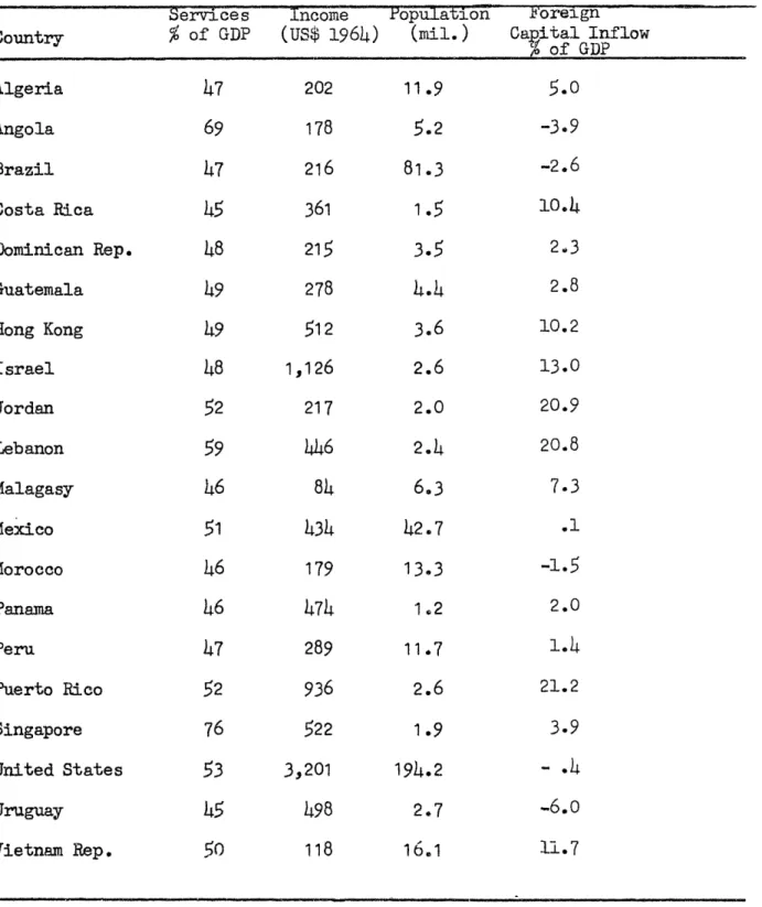
In Table 6 the 20 countries with a 1965 services share exceeding 45 per cent are listed together with their main characteristics MNost of the countries in the Table are small (the main exceptions are Brazil, Mexico,
and the U.S.); in 11 of them the population around 1965 was below five million. The countries in this group tend to depend heavily on foreign capital; in
seven of them the ratio of foreign capital to GDP exceeds 10 per cent. In three of the countries (Jordan, Lebanon., and Panama) exports of services account for over 10 per cent of GDP.
The Evidence
Annual Cross Sections. The hump in the income pattern of services is present in the cross section relations for both the full and the compatible
samples primarily for the 1950's. (Table 3 above). There is however a smaller degree of curvature in the compatible samples, and at a low income level there appears to be a prevalent and significant upward saift which is
bsent from the maximal samples. Both differences are d-ue to the fact that low income countries are excluded from the compatible sample because of lack of enough observations and to the differential time shifts as between income groups
discussed above (see also Table A8). The preceding section pointed out the relatively high share of industrial and primary production in the countrLes
-22-TABLE 6: High Services Countries Around 1965: Main Characteristics
ervices _Inoome ___opu1atJon Foreign
Country % of GDP (u,;$ 1964) (mil. ) Capital Inflow C of GDP Algeria 147 202 11.9 5.0 Angola 69 178 5.2 -3.9 Brazil 47 216 81.3 -2.6 Costa Rica 45 361 1.5 10.4 Dominican Rep. 48 215 3.5 2.3 Guatemala 49 278 4.4 2.8 Hong Kong 49 512 3.6 10.2 Israel 48 1126 2.6 13.0 Jordan 52 217 2.0 20.9 Lebanon 59 446 2.4 20.8 Malagasy 46 84 6.3 7.3 Mexico 51 434 42.7 .1 Morocco 46 179 13.3 -1.5 Panama 46 474 1.2 2.0 Peru
147
289 11.7 1.4 Puerto Rico 52 936 2.6 21.2 Singapore 76 522 1.9 3.9 United States 53 3,201 194.2 -.4
Uruguay 45 498 2.7 -6.0 Vietnam Rep. 50 118 16.1 11.7
-23-with lowest per capita income in 1965 in the sample. The counterpart of those high shares is, of course, a low figure for the share of services, and the fact that these countries enter the maximal samples gradually over time tends to increase the curvature and obscures any egogenous increase in services for the low income countries included.
Services in Large Countries. Since many of the countries with an extremely high share of services are small, a separate regression was run for the whole period for the large countries, defined as those countries where population in 1960 was at least 15 million. The estimated regression and the implied income pattern for a typical large country of 40 million population and capital
in-flow of two per cent appear on Figure 3.
The hump has now disappeared and the expected increase at high levels of income is confirmed.
Reduced Sanple of
34
Countries. As mentioned in the intro-duction to the paper, the dubious practice of leaving oi;t extremeobservations was avoided in this paper and in the Chenery and Syrquin (1975) study. In tbWs cas.% however, for illustration purposes we run a regression on 34 of the 42 countries in the compatible sample. The countries excluded were: Dominican Republic, Guatemala, Hong Kong3 Lebanon, Mexico, Panama, Peru and the U.S. (see Tablev6 for
their characteristics).
Since the poorer countries are not represented in this sample the variation was largely reduced but as can be seen from the results
N=40 F=.02 R2= .401 SEE = .0615 Vs = -.443 + .164 ly -. 0103(lY) 2 + .097 inN -.0099 (jnN)2 + .0383 F + .004 T1 + .002 T2 -`004T (4.0) (5-1 ) (3.8) (3.3) (2.8) (0.4) (0.4) (0.2) (0-5)3 e50-40 .oU RES -.30 .20 .10
i - L - I-L I I i 1 I I L I I I 1 i L I I I I I I ! I 1111 IItlIItiII
50 100 200 500 1000 1500 2000
-25-in Figure 4. exclud-25-ing the extreme countries does elim-25-inate the spurious reversal of the upward trend at the medium income level.
R 2= .165 N=1i0
SE= .05145 F= .02
.50
.40 - S'
3)4
CONTRIES
.30
v
116+.083 lX-.0O57(lnY) 2-_Q36 lnN+.OO77(lnN)2+e3576F(0.9) (2.0) (1.7) (4.9) (5.0) (8.4)
.20
.10
50
it0
0 2~0 0 Th000i5002J000Figure 4
The Time Series. The income elasticity within countries since 1950, in Table A9p is positive for most countries. The few with significant negative income elasticities are in almcst every case small countries in the medium income range, including several of the extreme countries listed in Table 6 (e.g., Hong Kong, Mexico, Panama and Singapore) or they are countries where the negative estimate is the result os an increasing share of services during a period when per capita income often contracted (Congo and Chad for example). On the other hand, the group of countries with highest positive elasticities includes several of the very low services countries (e.g., Honduras, Sudan$ Thailand and Zambia). It appears that countries with abnormally low or high share of services have been approaching the average normal values, while the rest have experienced a relative expansion in their output of services. These trends have brought about a compression of the intercountry variation in the
-26-share of services. The standard deviation of the share in 1950 for the 42 countries in the compatible sample was equal to .096, and over time it decreased muonotonically to .082 in 1955, .077 in 1960, and. o66 in 1965 in spite of the general increase in the value of the share (the coefficient of variation therefore falls even more). In the full samples the standard deviation increases for a while, as the low income - low services countries are added, but then declines. It was .096 in 1950, .101 in 1960, and down again to .088 by 1965.
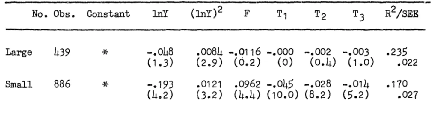
The average time series variation with income was presented in the previous section for both the full and the reduced total samples. Since the evidence presented so far suggests important differences associated with size as measutred by population, separatie short run patterns were also estimated for small and large countries, by letting each country have its own intercept. This procedure e:liminates the effect of variables with little or no variation over time and its results can therefore be identified as short run patterns, in contrast to the long run, cross section patterns, where the between countries variation plays a dominant role. The short run average estimates for small and large countries are given in Table 7. The pooled results were presented in Table
5.
The results show a tendency for the share to go up, the rate of increase being highest at high income levels (this follows from the positive sign of the quadratic income variable), In the results fQr the small countries and for the whole group there is first a falling stage, within the relevant income range, due to the decline toward a more normal value, in some of the small, medium income countries mentioned above. For large countries only, the results
-27-TABLE 7: Short Run Patterns of Services: Large Countries-Small Countries
No. Obse Constant MY ( )2 F T T2 T3 R2/SEE
Large 439 * -. 048 .0084 L. 0116 -. 000 -.002 -. 003 .235
(1.3) (2.9) (0.2) (0) (0.4) (1.0) .022 Small 886 * -.193 .0121 0962 -.045 -. 028 -. 014 .170
(4.2) (3.2) (4L4) (10.0) (8.2) (5.2) .027
* Each country has a d:ifferent intercept. t ratios in parentheses
A Very Brief Digression on Relative Prices.
The main result of the last section is the robustness of the positive association of the share of services with the level of development.
Apparent inconsistencies were seen to be the result of transient peculiar conditions in a few countries. Some writers however, have suggested that the positive income elasticity in cross section studies may be due to a price effect, since services are relatively underpriced in poor countries, or overpriced in rich countries. (Balassa, 1961). Since the evidence from the time series just presented is relatively free of this distortion,
3.7/
it appears then that Balassals conclusion that "theClark hypothesis of a rising tertiary sector ... does not stand up in the liglht of infomation on cross section data" (1961, p.397) does not stand up itself in the light of the available cross section data for the 1950-70 period.
-28-Concluding Remarks.
The main conclusion of this paper is that in cross country comparisons
the composition of the sample may largely determine the results. Cross sections based on one observation for each country are useful but have to be supplemented by information on the temporal stability of the underlying
relations. Reducing the sample by an extraneous criterion might be indicated at times but ornly if the criterion itself has theoretical underpinings.
Thus, in Chenery and Syrquin (1975) for example, alternative development patterns are estimated for groups of countries stratified by size and trade orientation, based on predictions from the theories of balanced growth and dynamic comparative advantage. In contrast, the estimation of regional relations, often found in empirical studies, are of limited significance for countries outside the region, or as "fstylized facts" on which a theory of development might once rest. In the past limited samples were often the inescapable result of the dearth of data. The rapid development of statistical knowledge in LDC's in the last two decades, though it still leaves much to be
FOOTNOTES
* For their competent research assistance I would like to thank Hazel Elkington and Dave Wermer.
1/ As a first approximation the observed patterns of resource allocation can be regarded as being the result of changes in demand with rising income and differences in trade patterns, resulting from variations in market size as well as changes in factor proportions. On these assumptions, an interindustry model yields solutions for levels of
consumption, production, and trade by sector as a function of the level of per capita GDP and population. (Chenery, 1965)
g/ Kuznets also cautioned against a mechanical application of cross section results to time series projections.
2 International Standard Industrial Classification. This particular grouping of sectors adopted in Chenery and Syrquin (1975) differs slightly from Kuznets'. Mining is grouped with agriculture since both are largely determined by natural resource endowments, and
utilities are treated separately since their output is not traded and are much more capital intensive than other services.
j1 Equation 1 was developed by testing the usefulness of alternative formulations to a variety of processes. Chenery (1960) used the form lnx =0a t+ PlnY +YlnN for the study of production patterns. A nonlirpar income term was added in Chenery and Taylor (1968). i/ For a simple statement of the adding-up criterion see Nicholson
(1957).
/
Most of the results for the utilities appear in Chenery and Syrquin (1975)./
No cross secbion equation was estimated for 1970 since only 21observations were available. These were included in the regressions for the whole period.
pooling may still be desirable in order to obtain an average estimate for the various groups, as in the text below.
2/
Only countries with at least five annual observations were included. jS The range between $100 and $1000 per capita income was chosen inChenery and Syrquin (1975) to represent the transition.
1l/
The estimated valuaes of the sector shares, when population equals 10million and with normal capital inflow for each level of income, are plotted for all income levels between $100 and $1000, Average actual values are also given for countries below $100 and above $1000 per capita
in-come, and connected by dashed lines to the regression results. The averages for the rich and poor countries approximate the upper and lower asymptotes which the present functional form cannot estimate. ig/ A first order autoregressive pattern of the residuals, for example, if similarly applicable to all countries, would have been absorbed by the time variables without impairing the properties (minimum variance , unbiased) of the least squares estimators.
LV The value of $500 was chosen to classifY countries by level of development following early tests with alternative values. As there are not many countries around this level, it was easy to identify two groups. The main results are not much influenced by small changes in the dividing value.
4J/
Such regressions are the basis of extensive cross section versus time series comparisons in Chenery and Syrquin (1975). The size variables are omitted since over a 10 to 20 year period population varies very little within countries.L5/
The function reaches a max-imum (or minimum) value with respect to income when TnY - 3/ 2 P2, whereP
1 andP 2 were defined aboveas the coefficients of the linear and the quadratic income terms respectively.
16/ There are over 20 countries in this range for which the relation was estimated (Table A9). In only one (Argentina) the income elasticity is negative. Due to the small size of the samples the quadratic term was omitted from the regressions.
17/ Balassa (1964) and Samuelson (1964) argue convincingly that the relative-price-of-services effect can also be found within a country over time. Over a 20-year period, however, it is most unlikely that it could by itself account for the significant increase in the share
of services. For a more extensive discussion on relative prices and
on exchange-rate conversions see the technical appendix in Chenery and Syrquin (1975).
BIBLIOGRAPHY
Balassa, B. 1961. Patterns of Industrial Growth: Comment. American
Economic Review. 51 (June): 394-97.
1964. The Purchasing-Power Parity Doctrine: A Reappraisal. Journal of Political Economy. 72 (December): 584-96
Chenery, H.B. 1960. Patterns of Industrial Growth. American Economic Review. 50 (September): 624-54.
- _ - 1965. The Process of Industrialization. Paper presented
to the First World Congress of the Econometric Society, Rome.
, and M. Syrquin. 1975. Patterns of Development, 1950-1970 London: Oxford University Press. 1975.
, and L. Taylor. 1968. Development Patterns: Among Countries and Over Ti-.'. Review of Economics and Statistics. 50 (November):
391-416.
Clark, Colin. 1940 (2nd ed. 1951, 3rd ed. 1957). The Conditions of Economic Progress. London: Macmillan.
Fisher, A.G.B. 1939. Production, Primary, Secondary and Tertiary. Economic Record. 15 (June): 24-38.
Johnston, J. 1972. Econometric Methods 2nd edn. New York:
McGraw-Hill.
Kuznets, S. 1957. Quantitative aspects of the economic growth of nations, II: Industrial distribution of national product and labor Force. Economic Development and Cultural Change, vol.5, July, suppl.
_ 1971. Economic Growth of Nations: Total Output and Production
Structure. Cambridge: Belknap Press of Harvard University Press.
Nicholson, J.L. 1957. The General Form of the Adding-Up Criterion. Journal of the Royal Statistical Society. (Series A - General) vol. 120, Part 1, pp. 84-85.
Samuelson, P.A. 1964. Theoretical Notes on Trade Problems. Review of
TABLE Al: Basic Dats 1965 or Closest Available Year
1 2 3 4
Income Year of
No. of Per Capita (Y) Population (N) Entry Into
Country Observations (1964-us$) (mnillions) Sample
* Algeria 21 202.4 11.9 1950 Angola 11 178.0 5.2 1953 * Argentina 20 786.6 21.7 1950 * Australia 19 168o.4 11.4 1950 * Ausxria 18 1052.3 7.3 1950 * Belgium 19 1538.0 9,5 1950 Bolivia 13 121240 4.3 1958 * Brazil 19 216.3 81.3 1950 Cambodia (Khmer) 8 101.8 6.5 1962 * Canada 18 2056.7 19.6 1950
Ceylon (Sri Lanka) 12 141.8 11.2 1959
Chad 11 58.5 3.3 1956 * Chile 19 4148.7 8.7 1950 * China (Taiwan) 20 201.0 12.14 1950 * Colombia 20 227.9 18.0 1950 Congo (Zaire) 114 71.0 16.14 1950 * Costa Rfica 18 360.7 1.5 1950 Dahomey 5 72. 2.4 1959 * Demnark 19 1727.1 4.8 1950 * Dominican Republic 21 215.4
3.5
1950 * Ecuador 20 195.3 5.2 1950 El Salvador 12 2140.5 2.9 1958 Ethiopia 9 51.6 22.7 1961 * Finland 19 1485.9 4.6 1950 * France 20 1705.7 48.8 1950 * Germany (West) 19 1613.7 59.0 1950 * Greece 20 585.0 8.5 1950 * Guatemala 20 277.9 4.4 1950 Haiti 12 80.4 4.4 1959 * Honduras 19 207.4 2.2 1950 * Hong Kong 21 511.8 3.6 1950 India 10 83.9 480.9 1960 Indonesia 12 83,8 1014.9 1958 Iran 12 217.8 24.8 1959 Iraq 15 2149.2 8e1 1953 Israel 17 1126.2 2,6 1953 * Italy 20 980.1 51.6 1950 Ivory Coast 11 178.7 4.3 1960 * Jamaica 20 419.7 1.8 1950 * Japan 20 780.4 980o 1950 Jordan 8 216.7 2,0 1959TABLE Al (Continued) 1 2 3
4
Country Kenya 7 95.5 9.6 1963 Korea (South) 18 123.4 28.4 1953 * Lebanon 19 446.4 2.4 1950 Liberia 5 179.3 1.1 1964 Libya 7 695.0 1.6 1962 Malagasy 6 84.4 6.3 1953 Malawi 7 57.5 3.9 1964 Malaysia 8 258.1 9.4 1960 Mali 13 57.0 4.5 1956 * Mexico 21 434.2 42.7 1950 Morocco 18 179.1 13.3 1952 * Netherlands 19 1335.4 12.3 1950 New Zealand 9 1806.4 2.6 1950 Nicaragua 11 330.3 1.7 1958 Niger 5 72.9 3.5 1961 Nigeria 17 87.8 48.7 1950 * Norway 19 1608.9 3.7 1950 Pakistan 11 84.3 113.9 1960 * Panama 19 474.4 1.2 1950 Papua 7 168.O 2.1 1961 * Paraguay 20 200.1 2.0 1950 * Peru 19 288.7 11.7 1950 * Philippines 21 149.3 31.8 1950 * Portugal 20 361.1 9.2 1950 * Puerto Rico 20 935.8 2.6 1950 Rhodesia 11 199.84.5
1960 Saudi Arabia 5 270.8 6.8 1963 Senegal 10 192.7 3.5 1959 Sierra Leone 6 134.9 2.4 1963 Singapore 11 522.2 1.9 1960 * South Africa 20 552.2 17.9 1950 Spain 16 572.2 31.6 1954 Sudan 14 87.8 13.7 1956 * Sweden 18 2242.7 7.7 1950 Syria 8 173.6 5.2 1963 Tanzania 9 67.1 11.7 1960 * Thailand 20 110.4 31.0 1950 Tunisia 11 198.04.4
1960 * Turkey 21 244.3 31.1 1950 Uganda 9 82.9 8.7 1961 UAR (Egypt) 15 137.7 29.4 1954TABLE Al (Continued) 1 2 3 4 Country * United Kingdom 20 1534.4 54.4 1950 * USA 19 3200.7 194.2 1950 Uruguay l5 497.5 2.7 1955 * Venezuela 20 829.6 8.7 1950 Vietnam (Souath) 6 117.7 16.1 1960 * Yugoslavia 21 414.8 i19.5 1950 Zambia 13 178.8 3.7 1954 No. of Obs. 1325
Table A2
PRIMAY PRODUCTION - FULL SAMPIE,
19'50 45 ob.
iPRI R*e2/SEE LY LYSO LOGN LNSO F CONSTANT
OLS U,6122 -0,5752 0,3995E-01 -0.6002E-02 -0.20942-02 0.11,352-01 2.274
OWss****. 0,9223E-01 -3.130 2,569 -0.1716 -0.2784 0.5640E-01 41,185
1951 14 obs
2 PRI R**2/SEE LY LYSO LOGN LNSO F CONSTANT
OLS 0.6478 -0,5974 0.4104E-01 0,1461E-01 -0.5853E-02 -0,1015 2,352
DW:e**** 0,9048E-01 -3,098 2,505 0,4211 -0.7915 -0.4851 4.148
1952 16 Obs
3 PR! R**2/SEF LY LYSO LOUN LNSO F CONSTANT
OLS 0,6679 -0.5560 0.3792E-OA -0,9118E-04 -0,4625E-02 -0.3524 2.247
OWs*a 0.8071E-01. -3,295 2,666 -0,2943E-02 -0.7003 -1,698 4,511
1953 60 Obs
4 eRI R**2/SEE LY LYSO LOGN LNSO F CONSTANT
OLS 0.7396 -Q.5046 0,3231E-01 0,1915E-02 -0,.5910E-02 -0,5591 2,138
DW:=***** 0,7802E-01 -3,163 2.391 0,6308E-01 -0.6129 -3.504 4.543
1951 53 Obs
5PR! R**2/SEE LY LYSO LOOGN LNSQ F CONSTANT
OLS 0,7733 -0.4461 0.2848E-Oi -0.1862E-01 -0.1244E-02 -0,7732 1.953
OWSe***-* 0.7216E-01 -3.052 2.320 -0,,6677 -0,2106 -5,959 4.510
19656 54 Obs
6 PRI R*@2/SrE2 LV LYSO LOGN LNSO F CONSTANIT
OLS 0,8041 -0,5527 0,36540-01 -0,22352-01 0.1730E-03 -0,6731 2,295
OW:s***s 0,67962-01 -3,985 3,153 -0,8373 0.30802-01 -5,483 5.562
195 56 Obs
7 PRI R**2/SEE LV LYSO LOON LNSQ F CONSTANT
OLS 0,*8171 -0,5546 0, 36352-01 -0 ,F782E-02 -0.2505E-02 -0.6602 2.*299
DW=***** 0,7307E-01 -4.675 3,586 -0.3000 -0.4139 -4,591 6.663
1957 66 Obs
8 PR! R*-2/SEE LY LYSO LOON LNSO F CONSTANT
OLS 0,8030 -n,4835 0.29582-01 -0,8993E-02 -0.1860E-02 -0.5615 2.123
OW=e**-** 0.7319E-01 -3 ,969 2 ,8431 -0 ,297 0 - 0 .30 17 -3,.623 6,.0 06
1958 60 Obs
9 PR! R**2/SEE LV LYSO LOGN LNSO F CONSTANT
OLS 0,8351 -0,5105 0,31890-01 -0,18252-01 0.56462-03 -0.6019 2,196
OW=****s 0,65342-U1 -4,842 3,538 -0,7204 0,1101 -4.651 7.148
1959 66 Obs
10 PRI R**2/SEE LV LYSO LOON LNSO F CONSTANT
OLS 0,8425 -fl,4792 0,2977E-U1 -0.10364-01 -0.7721E-03 -O,6416, 2,072
DWsoe*** 0,64142-81 -4,979 3,626 -0,4056 -0.1500 '6,216 7,465
1960 75 Obs
11 PR! Rs*2/SEF LV LYSO LOGN LNSO F CONSTANIT
OL-S 0.8097 -0,5067 0.,31540-U1 -0.25500-02 -0,58570-03 -0,5792 2,155 OW=~***** 0,72472-bl -4,707 3,453 -0.1113 -0.1402 -5,413 6,843
1961 77 Cbs
±2 PR! R*.2/SEE LY LYSU LOON LNSQ F CONSTANT
CLS 0.7817 -nl.5159 0,3164E-01 -0.14992-01 0,78732-03 -0,4472 2,225
DWZ***.*~ 0,84712-01 -4,525 3.237 -0,5643 0.1635 -3,336 6.699
1962 78 Obs
13 PR! R**2/SL0E LV LYSO LOON LNSQ F CONSTANT
OLS 0,7572 -0,4799 0,20'3E02-1 -0.3375E-01 0.46472-02 -0,4767 2,127 OWseo**** 0,8727E-ti1 -4.059 2,854 -1,2113 0,9358 -3.603 6,117
1963 82 Cbs
14 PRI R5e2,'SEE LY LYSU LOON LNS'O F CONSTANT
OLS 0.7925 -0,5156 0,317O0-01 -0,4985E-01. 0.6966E-02 -0.6399 2,257
uw=.**** 0,82452-Cl -4,767 3,436 -1,948 1,506 -5.598 7.141
1964 86 Cbs
1 5 PH! R**2/SEFOO( LV LYSr OO LNSQ F CONSTANT
OLSq 0,7891 -0,4112 0,2341E-01 -0.68410-01 0,10142-01 -0,6999 1,964
DW=~**** 0.bS40E-01 -4,113 2,758 -2,799 2.269 -6,682 6.709
1965 86 Cbs
16 PR! R**2/SLE LY LYSO LOOiN LNSQ F CONSTANT
OLS 0,7904 -0,4735 0,2856E-01 -0,6109E-01 0.81552-02 -0,6618 2,144 OW.BiUE,883-01 -4,792 3,420 -2,526 1.855 -6.079 7.384
1966 86 Obs
17 Pk! R**2/SEE LV L'10O LOON LNSC F CONSTAN4T
OLS 0,7330 -(1.3688 0,21622-31 -0,58482-01l 0,84622-02 -0,650,3 1,876
Dwz****a 0,90852-01 -3.417 2,255 -2,143 1,729 -5,536 5.592
1967 81 Obs
18 PR! R-~2/SEE LY LYS0 LOON LNSOI F CONSTANT
OLS 0,7326 -3,3582 0,1913E-!!1 -0,6428E-0i 0,9957E-02 -0,6781 1.790
Ows*-*** 0.8869E-01 -3,236 2,068 -2.365 2.062 -5.078 5,441
1968 73 Cbs
19 PR! R-~2/SEE LY LYSO LOGN LNSO F CoNSTA11T
OLS n,7786 -0.3735 0,20651--01 -0,34262-01 0.52852-02 -0,9152 1.779
OW:e**ss 0,7708E-01 -3,461 2.285 -1,373 1.209 -6.736 5.574
1969 5 b
20 PR! R**2/SEE LY L-YSO LOON LOSO F CONSTANT
OLS 0.7608 -0.2352 0,88720-02 0.1877E-01 -0,71132-03 -0,3265 i.284
DW=~*e** U.7406E-0± -1.600 0.700± 0,6009 -0,1371 -1.786 3,009
21 PR! R~*2/SEF L,Y LYSO LOGN LNSQ F CONSTANT
OLS 0.8211 -0.5088 0,296bE-01 0.1218 -0,1845E-01 -0.87±6 2.02d
Table A3
PRINARY PRODUCTION - REDUCED SAMPLE i950
1 PRI R**2/SEE LY LYSO LOGN LNSU F CONSTANT
OLS (1.5004 -0.4371 0.2855E-01 -0,857DE-03 -0,2912E-02 0.7533E-02 1.856
DWze**e 0.9425E-01 -1.775 J,392 -0.2362E-01 -0.3736 G,3556e-Ol 2.520 1951
2 PRI R**2/SEE LY LYSO LOGN LNSQ F CONSTANT
OLS 0.5452 -0,5262 0,3532E-01 0,1775E-01 -0.6693E-02 -0.1155 2.134
DO;=N*e* 0,9159E-01 -2,152 1,739 0.5015 -0.6843 -n.5372 2.916
1952
3 PPF R**2/$SE LY LYSQ LOGN LNSO F CONSTANT
OLS 0.5753 -0.4529 0,29556-01 0,1712E-02 -0,46646-02 -0.3704 1,932
U 0,8363E-01 -?.C04 1,582 0.5213E-C1 -0.6985 -1.659 2.843
l953
4 PRI Re*2/SEF LY LYSO LOGN LfSQ F CONSTANT
OLS 0.6790 -e.4280 0,2624E-01 -0,3094E-02 -0.3566E-02 -0,6423 1.910
DOW***** 0.7301E-01 -2,101 1.567 -0,1058 -0.5805 -3.126 3.101
1954I
5 PRI RO*2/SEE LY LYSO LOGN LNSO F CONSTANT
OLS 0.7095 -0.3737 0.2246E-01 -0.1046E-01 -0.23366-02 -0.6118 1.723
DOWe**e* 0.6460E-01 -2.064 1,511 -0.3995 -0,4291 -3.415 3.139
1955
6 pPt R**2/SSF LY LYSO LOGN LNSO F CONSTANT
OLS 0.7301 -n,3951 0,2376E-01 -0.1534E-01 -0.11046-02 -0.6232 1.809
DW=*4*** 0,6361E-01 -2.169 1,599 -0.5824 -0.2040 -3.574 3.261
1956
7 PRI R**2/SEE LY LYSO LOGN LNSO F CONSTA.NT
OLS 0.7248 -3.3702 n,22056-01 -0,7625E-02 -0.2960E-02 -0,6662 1.714
flw-=***** 0,63436-01 -2.035 1,491 -0.2847 -0.5437 -3.756 3.089
1957
8 pRI R*02/SEE LI LYSO LOGN LNSO F CONSTANT
OLS 0,7544 -0,1976 0,7200E-02 -0.12576-g0 -0,1177E-02 -0.6474 1.230
OW=***** 0,5980E-01 -1,130 0,5073 -0.4873 -0.2265 -4,750 2.303
1958
9 PRI R4*2/SEE LY LYSQ LOGN LISL F CONSTANT
OLS 0.7492 -0.3348 0,1816E-01 -0,7591E-02 -0.2178E-02 -0.6636 1.639
DW-***** 0.599BE-01 -1.915 1,280 -0.2906 -0.4174 -4,36d 3.061
1959
10 PRI R**2/SEE LY LYSO LOGN LNSO F CONSTANT
OLS 0,7514 -0.324i 0,1759E-O1 -0,4272E-02 -0.2561E-02 -0,6039 1,584
oW=***** 0,5931E-01 -t. 48 1.243 -0.1614 -0.4890 -4.307 2.934
1960
11 PRI R*2/56E6 LY LYSC LOCN LNSO F CONSTANT
ILS (0,7465 -0.4186 0.24626-b1 O.198CE-01 -0.6953i-02 -0.3875 1.860
DW=*v** 0,62236-nl -,-198 1,624 0.7138 -1.263 -2,868 3.162
1961
12 PRI R**2/SE6 LY LYSr4 LOGN LNSO F CONSTANT
OLS 0(,7732 -0.4147 0,2444E-01 0.1105E-01 -0,54586-02 -0.4211 1.860
OW:e*e*-P O.5901E-01 -?.306 1,700 0.4138 -1,041 -3.364 3.340
1962
13 PRI R**2/SEE LY LYSO LOON LNSO F CONSTANT
OLS 0.832P -C.4905 o30n96-01 -0.1021E-01 -0.1619E-02 -0,6720 2.133
D0w=e**e 0.5088E-01 -3.169 2,442 -0.4301 -0.3517 -5.277 4,418
1963
14 PRI *42/6SEE LY LYSO LOGN LNSQ F CONSTANT
OL 0.8099 -0.4478 0,2683E-01 -0,1717E-01 -0.6382E-03 -0.7257 2.004
U0W***** U.5281-01 -2,754 2,081 -0.6784 -0.1315 -4.687 3,941
1964
15 PR[ R**2/SEE LY LYSO LOGN LNSO F CONSTANT
OLS 0.6120 -0.3328 0,1'i19E-01 -Q,1364E-01 -0,1704E-02 -0.7757 1.632
DWZ***ee 0,5113E-01 -2.136 1.483 -0.5431 -0.359R -4.833 3,337
1965
16 PRI R-u/S6F. LY LYSO LOK>:N LNSU F CONSTANT
OLS 0,7961 -11,4045 0,2374E-01 -0,9797E-02 -0.2365E-02 -0.6188 1.851
Dh='*G 0,5390E-0l -2.456 1,838 -0,3683 -Q,4736 -3.617 3.567
1966
i7 PRI R**2/Sek LY LYSO LOGN LNSQ F CONSTANT
OLS 0,7947 -0.4500 0,2717F-C1 -0.2592E-02 -0,3183E-02 -0.545i 1.982 owz***** 0.5484E-Oi -2,623 2.030 -0,9323t-01 -0,6i34 -3.162 3.654 1967
18 PRI R**2/SE8 LY LYSO LOGN LNSO F CONSTANT
OLS 0,7766 -0.4263 0.2495F-01 0,8539E-03 -0.3073E-02 -0,6831 1.913 DW-*e*e 0,5573E-01 -2,434 1,831 C,2974E-01 -0.5769 -2.942 3.434
TABLE A4
INDUSTRY PRODUCTION - FULL SAMPLE
1950 45 Obs.
1 IMP R**2/SEE LI IESQ ICON UIQ F CONSTANT
OTS 0.67o1 0.2939 -o2841E-ol o.6843E-01 -0.90538-02 0.7733E-01 -0.9035
0W*** .6414E-01 2.299 -1.702 2.813 -1.730 0.15527 -2.391
1951 44 Cbs.
2 IMP R*+2,/SEE IF LYSQ ICOGN INSQ F CONSTANT
oWs 0,6425 0.2827 -0.1684E-01 0.5831E-01 -0.7598E,-02 0.1349E-01 0.8811
Dw=s-ws*s 0.6943E-01 1.911 -1.339 2.190 -1.339 0.8398E-01 -2.025
1952 46 Cbs.
3 IMP R**2/SEE IF LTYSQ LOGN LNSQ F CONSTANT
OIS 0.6143 0.2952 -0.1833E-01 0.5628E-01 -0.6780E-02 -0.5o64E-01 -0.9063
0w=s*s** o.6768E-01 2.086 -1.537 2.167 -1.224 -0.2909 -2.170
50 Cbs. 1953
4 IMP R*s2/SEE LI MOS COGN TINSQ F CONSTANT 018 0.6919 0.2843 -o.1631E-01 o.4779E-01 -0.5346E-02 0.1850 -0.'9134
Dw=***** o.6340E-01 2.193 -1.486 1.938 -1.032 1.427 -2.389
53 Cbs.
1 954
5 IMP R**2/SEE LI IFYSQ LWGN LNSQ F CONSTANT
Cr18 0.6843 0.2851 -o.166oE-ol o.5670E-01 -0.6891E-02 0.1960 -0.9181
oW**- .6359R.-0l 2.214 -1.534 2.308 -1.325 1.714 -2.4o6
54 Cbs. 1955
6 IMP R**2/SEE LI LYSQ WON I2ISQ F CONSTANT
018 0.7166 0.294o -0.1701E-01 o.6575E-ol -o.6820E-02 0.1536 -o.9649
oW=s***-s* o.6oo6E-O1 2.399 -1.661 2.787 -1 .777 1.415 -2.646
1956 56 Cbs.
7 IND. RX*2/63iLE LI IFTSQ LOGN WiSQ F CONSTANT
018 0.7207 0.2165 -0.1088E-01 0.5439E-01 -0.7026E-02 0.1235 -0.7093
I0w=***** 0.6136E-0l 2.174 -1.279 2.213 -1.383 1.023 -2.448
1957 55 Cbs.
8 IND R**2/SEE IF LEYSQ LOGN LRSQ F CONSTANT
CIS 0.7223 0.2015 -0.94538'-02 0.55888-0l -0 .7374E-02 o.140k -0.6763
DW=***s* 0.b01 E-01 2.012 -1.106 2.2 5 -1.455 1.102 -2.327
1958 60 Cbs.
9 IN0 R**2/SEE II LIYSQ LCOGN L-NSQ F CONSTANT
018 0.7274 0.2040 -0.9894E-02 0.80568-01 -0.8425E-02 0 925OE-01 -0.6761 Dw=s***s* 0:.57918E-C1 2.181 -1.237 2,694 -1.851 0.6055 -2.460
1959 66 Cbs.
10 IMP R**2/SEE LY LTSQ LOGN 18SQ F CONSTANT
018 0.7400 G.1660 -0.67768-02 o.6111E-02 -0.8429E-02 0.9693E-01 -0.5653
nw=***** 0.5658E-0l 1.955 -0.9356 2.713 -1.857 1,065 -2.309
1960 75 Obs.
11 IMP R**2/SEE LI LTSQ WOGN INSQ F CON1STANT
0T8 0.7249 0.1887 -0.82608-02 0.5212E-01 -0.60558-02 0.1371 -o.6475
Dw=***s* 0.6o34E-01 2.106 -i.o86 2.733 -1.741 1.539 -2.470
1961 77 Cbs.
12 180 R**2/SEE IF IZtSQ LONI I'NSQ F CONSTANT
018 0.73k3 0,1295 -0.3344E-02 o.5628E-01 -o.68k9E-02 0.1642 -o.k793
]N*** 0.5987E-01 1.607 -0.4839 2.997 -2,;013 1.733 -2.042
1962 78 Cbs.
13 rIMP R**2/SE8 LI IFSQ WONT INSQ F CONSTANT
018 0.7477 0.1412 -0.4301E-02 0.6394kB-Cl -0.8012E-02 0.1772 -0.5258
DW=*V**N* 0.5769E-01 1.806 -o.6445 3,k76 -2.441 2.025 -2.287
o2 Cbs. 1963
14 IMP R**2/SEE LI LYSQ WON LNSQ F CONSTANT
018 0.7579 0.1420 -o.4575E-02 0.6819E-ol -0.8705E-02 0.2657 -0.5273
ow**** 05647E-01 1.917 -0.72ko 3.890 -2.748 3.433 -2.436
86 Cbs.
196k ONIS FCNTN
15 IMP R:~-k-2/SEE LI LTSQ OISQFCNTT
018 O.77188 0.1075 -0.1949E-02 o.6952E-01 -0.9241E-.02 O.3036 -0.41 73 DW=+**s** 0.5353E-01 1.676 -0.3576 4.432 -3.223 4.516 -2.220
1965 85 Cbs. &TT
16 180 Rs-42/SEE LI IISQ LOON INSQ F CNTN
018 0.7632 0.1222 -0.32238-02 0.6608E-Cl -0.84628-02 0.26o6 -o.4565
Dw=-**sK-* 0.54988-01 1.840 -0.5744 4.067 -2.865 3.563 -2.340
1966 85 Cbs.
17 IN RIs*2/SEE LI LISQ LOON INSQ F CONSTANT
018 0,7527 0.1068 -0.19898-02 0.6801E-01 -0.90918-02 0.2930 -0.4090
ly 0 .5516E-ol 1.548 -0.3418 4.105 -3.060 4.1o8 -2.007
1967 81 Cbs
18 INDO R**2/Sg& LI LYSO L-OON LWNSQ F CONSTANT 018 0-7310 0.1160 -0,3067E-02 o.6659E-01 -0.9166E-02 0.3192 -0.4222 OW=-s-s* 0.5563E-Ol 1.670 -0.5286 3.906 -3.026 3.811 -2.047
1968 73 Cbs
19 IMP R**2/SEE LI LTS Q WON 1880Q F CONSTANT
018 0.7i26 0.1233 -0.3961E-02 0.5912E-01 -0.76368,-02 0.3549 -0.4213
Dw=**n** 0.54928-01 i.603 -0.6152 3.326 -2.451 3.666 -1.852
1969 53 Obs
20 18D R*s-2/SE8 LI L=S LOON 1880Q F CONSTANT 018 o.6484 O,177E-01 0.5232E-02 0.37078,-01 -0.418OE-02 0.2526 -0.9448E-01