Devavrat Shah
Department of Electrical Engineering and Computer Science, Massachusetts Institute of Technology, Cambridge, MA 02139, [email protected] Tauhid Zaman
Sloan School of Management, Massachusetts Institute of Technology, Cambridge, MA 02139, [email protected]
We consider the problem of detecting the source of a rumor which has spread in a network using only observations about which set of nodes are infected with the rumor and with no information as towhenthese nodes became infected. In a recent work (Shah and Zaman 2010) this rumor source detection problem was introduced and studied. The authors proposed the graph score functionrumor centralityas an estimator for detecting the source. They establish it to be the maximum likelihood estimator with respect to the popular Susceptible Infected (SI) model with exponential spreading times for regular trees. They showed that as the size of the infected graph increases, for a path graph (2-regular tree), the probability of source detection goes to0while ford-regular trees withd≥3the probability of detection, sayαd, remains bounded away from0and is less than1/2. However, their results stop short of providing insights for the performance of the rumor centrality estimator in more general settings such as irregular trees or the SI model with non-exponential spreading times.
This paper overcomes this limitation and establishes the effectiveness of rumor centrality for source detection for generic random trees and the SI model with a generic spreading time distribution. The key result is an interesting connec-tion between a continuous time branching process and the effectiveness of rumor centrality. Through this, it is possible to quantify the detection probability precisely. As a consequence, we recover all previous results as a special case and obtain a variety of novel results including theuniversalityof rumor centrality in the context of tree-like graphs and the SI model with a generic spreading time distribution.
Key words: rumors, networks, source detection, information diffusion History:
1. Introduction
Imagine someone starts a rumor which then spreads through a social network. After the rumor has spread for a long amount of time, we observe this network of rumor infected individuals. We only know who has heard the rumor and the underlying network structure. No information is given aboutwhenthe people heard the rumor. Our goal is to use only this information to discover the source of the rumor.
This rumor source detection problemis very general and arises in many different contexts. For exam-ple, the rumor could be a computer virus spreading through the Internet, a contagious disease infecting a human population, or a trend or new product diffusing through a social network. In each of these different
1
scenarios, detection of the source is of great interest. One would naturally like to find the originator of a malicious cyber-attack. Detecting the source of a viral epidemic would aid with the development of effec-tive vaccination, quarantine and prevention strategies. In social networks, sources of rumors, trends or new product adoption may be effective at disseminating information, and their identification would be of interest to companies wishing to develop viral marketing campaigns.
Detection of the source is made challenging in each of these situations by the fact that one may not have information regarding the time of the infection or adoption. For example, if the computer virus remains dormant and then upon activation renders the system inoperable, it may not be possible to determine when the machine was infected. For contagious diseases, determining exactly when a person became infected can be difficult due to lack of sufficient data. Rather, only a broad time window of when the infection occurred may be known. For trends or new product adoption one may be able to determine the exact time of adoption if this occurs through a social network such as Facebook which records the time of each user’s activity. However, there can be situations where people do not share the fact that they have adopted until much after they have done so, making it difficult to pinpoint precisely when the adoption occurred.
Given the wide ranging applications, it begs to understand the fundamental limitations of the source detection problem. Concretely, there are two key questions that need to be addressed. First, how does one actually construct the rumor source estimator? Since no information about infection times is given, a rumor source estimator would need to extract all information about the identity of the source using only the struc-ture of the rumor infected network, but it is not obvious in what manner. Second, what are the fundamental limits to this rumor source detection problem? In particular, how accurately can one find the rumor source, what is the magnitude of errors made in this detection, and how does the network structure affect one’s ability to find the rumor source?
1.1. Related Work
Rumor spreading was originally studied in the context of epidemiology in order to predict, control, and prevent the spread of infectious diseases. The epidemiological models for the spread of disease generally consisted of individuals that could be in one of three states : susceptible, infected, or recovered. In the susceptible-infected-recovered or SIR model all three states are allowed, but there are variants such as the SI model which only consider susceptible and infected individuals. Daniel Bernoulli developed the first differential equation models for the spread of a disease (Bernoulli and Blower 2004). Modern differential equation models were introduced in (Kermack and McKendrick 1927) and later expanded in (Anderson and May 1979a) and (Anderson and May 1979b). These models provided insight into the disease spreading dynamics, but they were very coarse and made several simplifying assumptions about human populations. The next level of modeling involved taking into account the network over which the disease spread. Contact network modeling was able to capture in greater detail the specific manner by which disease spread. These
models have allowed researchers to understand how the network structure affects the ability of a disease to become an epidemic (Moore and Newman (2000), Pastor-Satorras and Vespignani (2001), Ganesh et al. (2005)). The insights obtained from modeling disease spreading at a network level have allowed epidemi-ologists to develop vaccination and quarantine strategies to control modern viral epidemics (Meyers et al. (2003), Meyers et al. (2005), Pourbohoul et al. (2005), Pourbohoul et al. (2009), Bansal et al. (2006), Bansal et al. (2010), Fraser et al. (2009), Yang et al. (2009)).
The network models developed for disease propagation have found application in the context of online social networks. In Domingos and Richardson (2001), Kempe et al. (2003), and Hartline et al. (2008) optimization methods were applied to network models to select the best set of users to seed with a new product or information in order to maximize its spread in a social network. This work is complementary to that in epidemiology, where the goal is to prevent the spread of a viral outbreak, not accelerate it. Another interesting line of work has focused on using the spread of rumors in a social network to reconstruct the unknown network structure (Gomez-Rodriguez et al. (2010), Myers and Leskovec (2010), Netrapalli and Sanghavi (2012)).
Controlling the spread of a rumor, whether it be a contagious disease or the adoption of a new product, has been the main focus of a large amount of research, but the question of identifying the source of the rumor has been largely overlooked. A problem located at the intersection of probability theory and information theory recently emerged which is thematically related to rumor source detection. It is known as thereconstruction problem and the goal is to estimate the information possessed by a source based on noisy observations about this information as it propagates through a network. There are interesting similarities between the two problems: the signal of interest, the information of the source (for the reconstruction problem) and the rumor source itself (for the rumor source detection problem) are extremely ‘low-dimensional’. However, the observations for each problem, the noisy versions of the information (reconstruction) and infected nodes (rumor source detection), lie in a very ‘high-dimensional’ setting. This makes estimation and detection quite challenging. It is not surprising that results for the reconstruction problem, even for tree or tree-like graphs, have required sophisticated mathematical techniques (Evans et al. (2000), Mossel (2001), Gerschenfeld and Montanari (2007)). Therefore, one would expect similar types of challenges for the rumor source detection problem, which involves not estimating information at a known source, but rather finding the source itself among a large number of vertices in a network.
The rumor source detection problem was first formally posed and studied in Shah and Zaman (2010). The authors proposed a graph-score function calledrumor centralityas an estimator for the rumor source. They showed that the node with maximal rumor centrality is the maximum likelihood (ML) estimate of the source for rumor spreading on regular trees under the SI model with homogeneous exponential spreading times. They demonstrated the effectiveness of this estimator by establishing that the rumor source is found
with strictly positive probability for regular trees and geometric trees under this setting. The model and precise results from Shah and Zaman (2010) are described in Section 2.
While this work laid the foundations of the rumor source detection problem, the results had some key limitations. First, they do not quantify the exact detection probability, sayαd, ford-regular graphs, for the proposed ML estimator other thanα2= 0, α3= 0.25 and0< αd≤0.5 for d≥4 for the SI model with
exponential spreading times. Second, the results do not quantify the magnitude of the error in the event of not being able to identify the source. Third, the results do not provide any insights into how the estimator behaves for rumor spreading on generic heterogeneous tree (or tree-like) graphs under the SI model with a generic spreading time distribution.
1.2. Summary of Results
The primary reason behind the limitations of the results in Shah and Zaman (2010) is the fact that the analytic method employed there is quite specific to regular trees with homogeneous exponential spreading times. To overcome these limitations, as the main contribution of this work we introduce a novel analysis method that utilizes connections to the classical Markov branching process (MBP) (equivalently, a general-ized Polya’s urn (GPU)). As a consequence of this, we are able to quantify the probability of the error event precisely and thus eliminate the shortcomings of the prior work.
Our results in this work collectively establish that, even though, rumor centrality is an ML estimator only for regular trees and the SI model with exponential spreading times, it is universally effective with respect to heterogeneity in the tree structure and spreading time distributions. It’s effectiveness for generic random trees immediately implies its utility for finding sources in sparse random graphs that are locally tree-like. Examples include Erdos-Renyi and random regular graphs. A brief discussion to this effect can be found in Section 3.4.
The following is a summary of our main results (see Section 3 for precise statements): 1. Regular trees, SI model with exponential spreading times:
We characterizeαd, the detection probability ford-regular trees, for alld. Specifically, ford≥3
αd=dI1/2 1 d−2, d−1 d−2 −(d−1).
In above Ix(a, b) is the incomplete beta function with parameters a, bevaluated atx∈[0,1] (see (3.1)). This implies that αd >0for d≥3, α3= 0.25, andαd→1−ln 2 asd→ ∞. Further, we show that the
probability of rumor centrality estimating thekthinfected node as the source decays asexp(−Θ(k)). The precise results are stated as Theorem 3.1, Corollaries 1 and 2.
2. Generic random trees, SI model with exponential spreading times: For generic random trees (see Section 3.2 for precise definition) which are expanding, we establish that there is strictly positive probability of correct detection using rumor centrality. Furthermore, the probability of rumor centrality estimating the
kthinfected node as the source decays asexp (−Θ(k)). The precise results are stated as Theorem 3.2 and Theorem 3.3.
3. Geometric trees, SI model with generic spreading times:
For any geometric tree (see Section 3.2.2 for precise definition), we establish that the probability of correct detection goes to1as the number of infected nodes increases. The precise result is stated as Theorem 3.4.
4. Generic random trees, SI model with generic spreading times:
For generic expanding random trees with generic spreading times (see Section 3.2 for definition), we establish that the probability of correct source detection remains bounded away from0. The precise result is stated as Theorem 3.2.
2. Model, Problem Statement and Rumor Centrality
We start by describing the model and problem statement followed by a quick recall of the precise results from Shah and Zaman (2010). In the process, we shall recall the definition of rumor centrality and source estimation as introduced in Shah and Zaman (2010).
2.1. Model
LetG= (V,E)be a possibly infinite connected graph. Letv∈ Vbe a rumor source from which a rumor starts spreading at time0. As per the classical Susceptible Infected (SI) model the rumor spreads in the graph. Specifically, each edgee= (u1, u2) has a spreading timeSeassociated with it. If nodeu1gets infected at
timet1, then at timet1+Sethe infection spreads fromu1tou2. A node, once becoming infected, remains
infected. The spreading times associated with edges are independent random variables with identical distri-bution. LetF:R→[0,1]denote the cumulative density function of the spreading time distribution. We shall
assume that the distribution is non-negative valued, i.e.F(0) = 0and it is non-atomic at0, i.e.F(0+) = 0.
Since it is a cumulative density function, it is non-decreasing andlimx→∞F(x) = 1. The simplest, homo-geneous SI model has exponential spreading times with parameterλ >0withF(x) = 1−exp(−λx) for x≥0. In Shah and Zaman (2010), the results were restricted to this homogeneous exponential spreading time setting. In this paper, we shall develop results for arbitrary spreading time distributions consistent with the above assumptions.
Given the above spreading model, we observe the rumor infected graph G(t) = (V(t), E(t)) at some time t >0. To simplify our notation, we will refer to the time dependent rumor infected graph at timet simply asG= (V, E). We do not know the value oft or the realization of the spreading times on edges e∈E; we only know the rumor infected nodesV ⊂ V and edges between themE=V ×V ∩ E. The goal is to find the rumor source (amongV) givenG.
We note here that in this setting we do not observe the underlying graphG. This means we do not observe edges on the boundary between infected and non-infected nodes. However, these boundary edges do pro-vide additional information. For example, if an infected node has a large number of uninfected neighbors, then it is likely that this node has not been infected for very long, otherwise more of its neighbors would be infected. Intuitively, this would mean that it is less likely that this node is the source. Our rumor source esti-mator, which we present next, does not require any knowledge ofG, though our analysis of the estimator’s performance will require knowledge of the structure ofG. We will find that without observingG, our rumor source estimator is still able to perform well on a variety of graphs under general spreading models.
2.2. Rumor Centrality: An Estimator
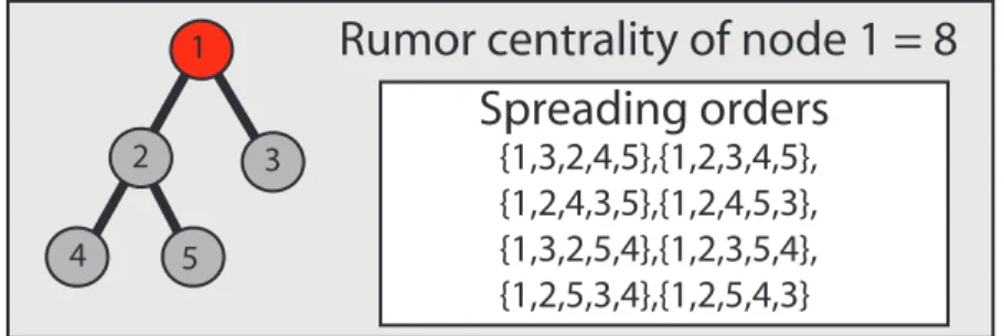
To solve the rumor source detection problem, the notion of rumor centrality was introduced in Shah and Zaman (2010). Rumor centrality is a ‘graph score’ function. That is, it takesG= (V, E)as input and assigns a non-negative number or score to each of the vertices. Then the estimated source is the one with maximal (ties broken uniformly at random) score or rumor centrality. The node with maximal rumor centrality is called the ‘rumor center’ (which is also the estimated source) with ties broken uniformly at random. We start with the precise description of rumor centrality for a tree1graphG: the rumor centrality of nodeu∈V with respect toG= (V, E)is R(u, G) =Q|V|! w∈VT u w , (2.1) where Tu
w is the size of the subtree of G that is rooted at w and points away from u. For example, in Figure 1, let u be node 1. Then|V|= 5; the subtree sizes are T1
1 = 5, T 1 2 = 3,T 1 3 =T 1 4 =T 1 5 = 1 and
henceR(1, G) = 8. In Shah and Zaman (2010), a linear time algorithm is described to compute the rumor centrality of all nodes building on the relationR(u, G)/R(v, G) =Tv
u/T u
v for neighboring nodesu, v∈V ((u, v)∈E).
The rumor centrality of a given nodeu∈V for a tree given by (2.1) is precisely the number of distinct spreading orders that could lead to the rumor infected graphGstarting fromu. This is equivalent to comput-ing the number of linear extensions of the partial order imposed by the graphGdue to causality constraints of rumor spreading. Under the SI model with homogeneous exponential spreading times and a regular tree, it turns out that each of the spreading orders is equally likely. Therefore, rumor centrality turns out to be the maximum likelihood (ML) estimator for the source in this specific setting (cf. Shah and Zaman (2010)). In general, the likelihood of each node u∈V being the source givenG is proportional to the weighted summation of the number of distinct spreading orders starting fromu, where weight of a spreading order could depend on the details of the graph structure and spreading time distribution of the SI model. Now
1
1
2 3
4 5
Rumor centrality of node 1 = 8
{1,3,2,4,5},{1,2,3,4,5}, {1,2,4,3,5},{1,2,4,5,3}, {1,3,2,5,4},{1,2,3,5,4}, {1,2,5,3,4},{1,2,5,4,3}
Spreading orders
Figure 1 Example of rumor centrality calculation for a5node network. The rumor centrality of node1is8because there are8
spreading orders that it can originate, which are shown in the figure.
for a tree graph and SI model with homogeneous exponential spreading times, as mentioned above, such a quantity can be computed in linear time. But in general, this could be complicated. For example, computing the number of linear extensions of a given partial order is known to be #P-complete (Brightwell and Win-kler (1991)). While there are algorithms for approximately sampling linear extensions given a partial order (Karzanov and Khachiyan (1991)), Shah and Zaman (2010) proposed the following simpler alternative for general graphs.
Definition 1 [Rumor Centrality] Given nodeu∈V in graphG= (V, E), letT⊂Gdenote a breadth-first search tree ofuwith respect toG. Then, the rumor centrality ofuwith respect toGis obtained by computing it as per(2.1)with respect toT. The estimated rumor source is the one with maximal rumor centrality (ties broken uniformly at random).
2.3. Prior Results
In Shah and Zaman (2010), the authors established that rumor centrality is the maximum-likelihood esti-mator for the rumor source when the underlying graphG is a regular tree. They studied the effectiveness of this ML estimator for such regular trees. Specifically, suppose we observe then(t)node rumor infected graphGafter timet, which is a subgraph ofG. LetCk
t be the event that the source estimated as per rumor centrality is thekth infected node, and thusC1
t corresponds to the event of correct detection. The following are key results from Shah and Zaman (2010):
Theorem 2.1 (Shah and Zaman (2010)) LetGbe ad-regular infinite tree withd≥2. Let
αL d = lim inft →∞ P C1 t ≤lim sup t→∞ PC1 t =αU d. (2.2) Then, αL2 =α U 2 = 0, α L 3 =α U 3 = 1 4, and 0< α L d ≤α U d ≤ 1 2, ∀d≥4. (2.3)
3. Main Results
We state the main results of this paper. In a nutshell, our results concern the characterization of the probabil-ity ofCk
t for anyk≥1for largetwhenGis a generic tree. As a consequence, it provides a characterization of the performance for sparse random graphs.
3.1. Regular Trees, SI Model with Exponential Spreading Times
We first look at rumor source detection on regular trees with degreed≥3, where rumor centrality is an exact ML estimator when the spreading times are exponentially distributed. Our results will utilize properties of Beta random variables. We recall that the regularized incomplete Beta functionIx(a, b) is the probability that a Beta random variable with parametersaandbis less thanx∈[0,1],
Ix(a, b) = Γ(a+b) Γ(a)Γ(b)
Z x
0
ta−1(1−t)b−1dt, (3.1)
whereΓ(·)is the standard Gamma function. For regular trees of degree≥3we obtain the following result.
Theorem 3.1 LetGbed-regular infinite tree withd≥3. Assume a rumor spreads onGas per the SI model with exponential distribution with rateλ. Then, for anyk≥1,
lim t→∞P Ck t =I1/2 k−1 + 1 d−2,1 + 1 d−2 + (d−1) I1/2 1 d−2, k+ 1 d−2 −1 . (3.2)
Fork= 1, Theorem 3.1 yields thatαL d =α
U
d =αdfor alld≥3where
αd=dI1/2 1 d−2, d−1 d−2 −(d−1). (3.3) More interestingly, Corollary 1 lim d→∞αd= 1−ln 2 ≈ 0.307. (3.4)
For any d≥3, we can obtain a simple upper bound for Theorem 3.1 which provides the insight that the probability of error in the estimation decays exponentially with error distance (not number of hops in graph, but based on chronological order of infection) from the true source.
Corollary 2 WhenGis ad-regular infinite tree, for anyk≥1,
lim t→∞P Ck t ≤k(k+ 1) 1 2 k−1 exp−Θ(k).
0 5 10 15 20 10−6 10−4 10−2 100 102
k (infection rank)
mil
tP
(
C
k t)
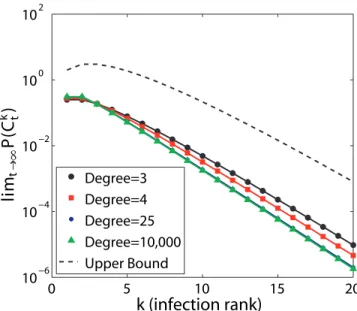
Degree=3 Degree=4 Degree=25 Degree=10,000 Upper Bound 8 Figure 2 limt→∞P Ctkversuskfor regular trees of different degree.
lim P(C
1)
n 8 nα
d 101 102 103 104 0 0.1 0.2 0.3 0.4 0.5Degree
1/4
1-ln(2)
Figure 3 αdversus degreedfor regular trees.
To provide intuition, we plot the asymptotic error distributionlimt→∞P(Ctk)for different degree regular trees in Figure 2. As can be seen, for degrees greater than4, all the error distributions fall on top of each other, and the probability of detecting thekthinfection as the source decays exponentially ink. We also plot the upper bound from Corollary 2. As can be seen, this upper bound captures the rate of decay of the error probability. Thus we see tight concentration of the error for this class of graphs. Figure 3 plots the asymptotic correct detection probabilityαd versus degreedfor these regular trees. It can be seen that the detection probability starts at1/4 for degree 3 and rapidly converges to1−ln(2)as the degree goes to infinity.
3.2. Generic Random Trees, SI Model with Generic Spreading Times
The above precise results were obtained using the memoryless property of the exponential distribution and the regularity of the trees. Next, we wish to look at a more general setting both in terms of tree structures and spreading time distributions. In this more general setting, while we cannot obtain precise values for the detection and error probabilities, we are able to make statements about the non-triviality of the detection probability of rumor centrality. When restricted to exponential spreading times for generic trees, we can identify bounds on the error probability as well. Let us start by defining what we mean by generic random trees through a generative model.
Definition 2 (Generic Random Trees) It is a rooted random tree, generated as follows: given a root node as a starting vertex, addη0children to root whereη0is an independent random variable with distribution D0. If η06= 0, then add a random number of children chosen as per distributionD over{0,1, . . .}
inde-pendently to each child of the root. Recursively, to each newly added node, add indeinde-pendently a random number of nodes as per distributionD.
The generative model described above is precisely the standard Galton-Watson branching process ifD0= D. If we take D0 andD to be deterministic distributions with support ondand d−1 respectively, then
it gives thed-regular tree. For a random d-regular graph on nnodes, as ngrows the neighborhood of a randomly chosen node in the graph converges (in distribution, locally) to such ad-regular tree. If we take D0=D as a Poisson distribution with mean c >0, then it asymptotically equals (in distribution) to the
local neighborhood of a randomly chosen node in a sparse Erdos-Renyi graph as the number of nodes grows. Recall that a (sparse) Erdos-Renyi graph onnnodes with parametercis generated by selecting each of the n2edges to be present with probabilityc/nindependently. Effectively, random trees as described above capture the local structure for sparse random graphs reasonably well. For that reason, establishing the effectiveness of rumor centrality for source detection for such trees provide insights into its effectiveness for sparse random graph models.
We shall consider spreading time distributions to be generic. Let F : [0,∞)→[0,1]be the cumulative distribution function of the spreading times. ClearlyF(0) = 0,F is non-decreasing andlimt→∞F(t) = 1. In addition, we shall require that the distribution is non-atomic at0, i.e.F(0+) = 0. We state the following
result about the effectiveness of rumor centrality with such generic spreading time distribution.
Theorem 3.2 Letη0, distributed asD0, be such thatPr(η0≥3)>0and letη, distributed as perD, be such
that1<E[η]<∞. Suppose the rumor starts from the root of the random tree generated as per distributions
D0andDas described above and spreads as per the SI model with a spreading time distribution with an
absolutely continuous density. Then,
lim inf t→∞ P C1 t >0.
The above result says that irrespective of the structure of the random trees, spreading time distribution and elapsed time, there is non-trivial probability of detecting the root as the source by rumor centrality. The interesting aspect of the result is that this non-trivial detection probability is established by studying events when the tree grows without bound. For finite size trees withnnodes, the rumor source can be estimated by selecting a random node, giving a probability of correct detection ofn−1>0. However, such events are
trivial and are not of much interest to us (neither mathematically, nor motivationally).
3.2.1. Generic Random Trees, SI Model With Exponential Spreading Times Extending the results of Theorem 3.2 for explicitly bounding the probability of the error eventP Ck
t
for generic spreading time distribution seems rather challenging. Here we provide a result for generic random trees with exponential spreading times.
Theorem 3.3 Consider the setup of Theorem 3.2 with spreading times being homogeneous exponential distributions with (unknown, but fixed) parameterλ >0. In addition, letD0=D. Letη, distributed as per D, be such thatE[η]>1andE[exp(θη)]<∞ for allθ∈(−ε, ε)for some ε >0. Then, for appropriate constantsC0, C00>0, lim sup t→∞ P Ctk ≤C0exp(−kC00). (3.5)
The above result establishes an explicit upper bound on the probability of the error event. The bound applies to essentially any generic random tree and demonstrates that the probability of identifying later infected nodes as the rumor source decreases exponentially fast.
3.2.2. Geometric Trees, SI Model With Generic Spreading Times The trees considered thus far, d-regular trees withd≥3or random trees withE[η]>1, grow exponentially in size with the diameter of the tree. This is in contrast with path graphs ord-regular trees withd= 2which grow only linearly in diameter. It can be easily seen that the probability of correct detection,P(C1
t)will scale asΘ(1/ √
t)for path graphs as long as the spreading time distribution has non-trivial variance (see Shah and Zaman (2010) for proof of this statement for the SI model with exponential spreading times). In contrast, the results of this paper stated thus far suggest that the expanding trees allow for non-trivial detection ast→ ∞. Thus, qualitatively path graphs and expanding trees are quite different – one does not allow detection while the other does. To understand where the precise detectability threshold lies, we look at polynomially growinggeometric
trees.
Definition 3 (Geometric Tree) A geometric tree is a rooted, non-regular tree parameterized by constants
α,b, and c, withα≥0,0< b≤c, and root nodev∗. Letd∗ be the degree ofv∗, let the neighbors ofv∗
i= 1,2, ..., d∗. Denote the number of nodes in Ti at distance exactlyr from the subtree’s root nodevi as ni(r). Then we require that for all1≤i≤d∗
brα≤ni(r)≤crα. (3.6)
The condition imposed by (3.6) states that each of the neighboring subtrees of the root should satisfy polynomial growth (with exponentα >0) and regularity properties. The parameterα >0characterizes the growth of the subtrees and the ratioc/bdescribes the regularity of the subtrees. Ifc/b≈1then the subtrees are somewhat regular, whereas if the ratio is much greater than 1, there is substantial heterogeneity in the subtrees. Note that the path graph is a geometric tree withα= 0,b= 1, andc= 2.
We shall consider the scenario where the rumor starts from the root node of a rooted geometric tree. We shall show that rumor centrality detects the root as the source with an asymptotic probability of 1 for a generic spreading time distribution with exponential tails. This is quite interesting given the fact that rumor centrality is an ML estimator only for regular trees with exponential spreading times. The precise result is stated next.
Theorem 3.4 LetG be a rooted geometric tree as described above with parametersα >0,0< b≤cand root nodev∗with degreed∗such that
dv∗>c
b+ 1.
Suppose the rumor starts spreading onGstarting fromv∗as per the SI model with a generic spreading time
distribution whose cumulative density functionF:R→[0,1]is such that (a)F(0) = 0, (b)F(0+) = 0, and (c) ifX is a random variable distributed as perF thenE[exp(θX)]<∞forθ∈(−ε, ε)for someε >0. Then
lim t P(C
1
t) = 1.
A similar theorem was proven in Shah and Zaman (2010), but only for the SI model with exponential spreading times. We have now extended this result to arbitrarily distributed spreading times. Theorem 3.4 says thatα= 0andα >0serve as a threshold for non-trivial detection: forα= 0, the graph is a path graph, so we would expect the detection probability to go to 0ast→ ∞as discussed above, but for α >0 the detection probability converges to1ast→ ∞.
3.3. Detection Probability and Graph Growth: Discussion
Our results can be viewed as relating detection probability to graph growth parametrized byα. For path graphs, where no detection is possible,α= 0. For any finite, positiveαwe have geometric graphs where the detection probability converges to one. For regular trees or random graphs, the growth is exponential, which givesα=∞, and we have a detection probability that is strictly between zero and one.
To understand these results at a high level, it is helpful to consider the properties of the rumor center given by Lemma 1. Essentially, this lemma states that the graph isbalancedaround the rumor center. For the rumor source to be the rumor center (and therefore correctly identified as the true source), the rumor must spread in a balanced way. For a path graph (α= 0), balance is a very delicate condition, requiring both subtrees of the source to be exactly equal in size. The probability of this occurring goes to zero as the graph size goes to infinity.
For any non-negative, finite alpha, this balance condition becomes easier to achieve if the source has degree greater than or equal to three. In this case, because the number of vertices grows polynomially, the variation of the size of a rumor infected subtree after a timetis much smaller than the expected value of its size, resulting in a concentration of the size. This means that with high probability, no subtree will be larger than half of the network size, and balance is achieved. The key here is that the boundary where the rumor can spread grows slower than the size of the rumor infected graph. If the graph has dα+1 nodes, then the
boundary containsdαnodes.
For infinite alpha, which corresponds to graphs with exponential growth, the rumor boundary size is of the same order of magnitude in size as the rumor infected graph. This results in a high variance in the subtree size. We would expect this high variance to result in detection becoming impossible. However, our analysis shows that the manner in which the rumor spreads on these graphs results in detection being possible with strictly positive probability. Another way to view this result is that the vertices in each subtree act as witnesses which we can use to triangulate the source. If there are three or more subtrees, and the subtree sizes do not vary considerably (as in graphs with polynomial growth), then the witnesses have low noise, and we can detect the source exactly as the observed rumor infected graph grows. For exponentially growing graphs, the noise in the signals provided by the witnesses grows with the number of witnesses. The increased number of witnesses balances the increased noise to give a detection probability that remains strictly positive as the graph size goes to infinity.
3.4. Locally Tree-Like Graphs: Discussion
The results of the paper are primarily for tree structured graphs. On one hand, these are specialized graphs. On the other hand, they serve as local approximations for a variety of sparse random graph models. As discussed earlier, for a randomd-regular graph overmnodes, a randomly chosen node’s local neighborhood (say up to distance o(logm)) is a tree with high probability. Similarly, consider an Erdos-Renyi graph overmnodes with each edge being present with probabilityp=c/mindependently for anyc >0(c >1 is an interesting regime due to the existence the of a giant component). A randomly chosen node’s local neighborhood (up to distanceo(logm)) is a tree and distributionally equivalent (in the largemlimit) to a random tree with Poisson degree distribution.
0 2 4 6 8 10 12 10−4 10−3 10−2 10−1 100
k (infection rank)
P
(
C
k 500)
c=10
c=20
Regular Tree Degree=10
Regular Tree Degree=20
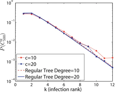
Figure 4 Empirical error probability versuskfor Erdos-Renyi graphs with 500 vertices, mean degree10and20, and exponen-tially distributed spreading times with mean one. Also shown arelimt→∞P Ctk
for degree10and20regular trees with exponentially distributed spreading times with mean one.
Given such ‘locally tree-like’ structural properties, if a rumor spreads on a random d-regular graph or sparse Erdos-Renyi graph for timeo(logm)starting from a random node, then rumor centrality can detect the source with guarantees given by Theorems 3.1 and 3.2. Thus, although the results of this paper are for tree structured graphs, they do have meaningful implications for tree-like sparse graphs.
For the purpose of illustration, we conducted some simulations for Erdos-Renyi graphs that are reported in Figure 4. We generated graphs withm= 50,000nodes and edge probabilitiesp=c/mforc= 10and c= 20. The rumor graph containedn= 500nodes and the spreading times had an exponential distribution with mean one. We used the general graph version of rumor centrality as defined in Definition 1 as the rumor source estimator. We ran 10,000rumor spreading simulations to obtain the empirical error distributions plotted in Figure 4. As can be seen, the error drops of exponentially ink, very similar to the regular tree error distribution. To make this more evident, we also plot the asymptotic error distributions for regular trees of degree10and20and it can be seen that the error decays at similar, exponential rates. This indicates that even though there is substantial randomness in the graph, the asymptotic rumor source detection error distribution behaves as though it were a regular tree graph. This result also suggests that the bounds in Theorem 3.3 are loose for this graph.
4. Proofs
Here proofs of the results stated in Section 3 are presented. We establish results for d-regular trees by connecting rumor spreading with Polya urn models and branching processes. Later we extend this novel method to establish results for generic random trees under arbitrary spreading time distributions. After this,
we prove Theorem 3.4 using standard Chernoff’s bound and the polynomial growth property of geometric trees.
4.1. Proof of Theorem 3.1:d-Regular Trees
4.1.1. Background: Polya’s Urn. We will recall Polya’s urn process and it’s asymptotic properties that we shall crucially utilize in establishing Theorem 3.1. An interested reader can find a good exposition in Athreya and Ney (1972).
In the simplest form, Polya’s Urn process operates in discrete time. Initially, at time0, an urn contains balls of two types, sayW0 white balls andB0 black balls. LetWnandBn denote the number of white and
black balls, respectively, at the end of timen≥1. At each timen≥1, a ball is drawn at random from the urn (Wn−1+Bn−1balls in total). This ball is added back along withα≥1new balls of the same type leading
to a new configuration of balls (Wn, Bn). For instance, at time n, a white ball is drawn with probability Wn−1/(Wn−1+Bn−1)and we have thatWn=Wn−1+α, Bn=Bn−1.
Under the above described process, it is easy to check that the fraction of white (or black) balls is a bounded martingale. Therefore, by the martingale convergence theorem, it has a limit almost surely. What is interesting is that the limiting distribution is nicely characterized as stated below.
Theorem 4.1 (Athreya and Ney 1972, Theorem 1, pp. 220) For the Polya’s Urn process described above
Wn
Wn+Bn →Y almost surely, (4.1)
whereY is a Beta random variable with parametersW0/αandB0/α. That is, forx∈[0,1],
P(Y ≤x) =IxW0 α , B0 α ,
whereIx(a, b)is the incomplete Beta function defined as in(3.1)
4.1.2. Setup and Notation. LetG= (V,E)be an infinited-regular tree and let the rumor start spreading from a node, sayv1. Without loss of generality, we view the tree as a randomly generated tree, as described
in Section 3, withv1being the root withdchildren and all the subsequent nodes withd−1children (hence
each node has degree d). We shall be interested in d≥3. Now suppose the rumor is spread on this tree starting fromv1as per the SI model with exponential distribution with rateλ >0.
Initially, nodev1is the only rumor infected node and itsdneighbors are potential nodes that can receive
the rumor. We will denote the set of nodes that are not yet rumor infected but are neighbors of rumor infected nodes as the rumor boundary. Initially the rumor boundary consists of the d neighbors of v1.
Under the SI model, each edge has an independent exponential clock of mean 1/λ. The minimum ofd independent exponentials of mean1/λis an exponential random variable of mean1/(dλ), and hence when
one of thednodes (chosen uniformly at random) in the rumor boundary gets infected, the infection time has an exponential distribution with mean1/(dλ). Upon this infection, this node gets removed from the boundary and adds itsd−1children to the rumor boundary. That is, each infection addsd−2new nodes to the rumor boundary. In summary, letZ(t)denote the number of nodes in the rumor boundary at timet, thenZ(0) =dandZ(t)evolves as follows: each of theZ(t)nodes has an exponential clock of mean1/λ; when it ticks, it dies andd−1new nodes are born which in turn start their own independent exponential clocks of mean1/λand so on. Letu1, . . . , ud be the children ofv1; letZi(t)denote the number of nodes
in the rumor boundary that belong to the subtreeTi(t)that is rooted atui with Zi(0) = 1 for1≤i≤d; Z(t) =Pd
i=1Zi(t). LetTi(t) =|Ti(t)|denote the total number of nodes infected in the subtree rooted atui
at timet; initiallyTi(0) = 0for1≤i≤d. Since each infected node addd−2nodes to the rumor boundary, it can be easily checked thatZi(t) = (d−2)Ti(t) + 1and henceZ(t) = (d−2)T(t) +dwithT(t)being the total number of infected nodes at timet(excludingv1).
4.1.3. Probability of Correct Detection. Suppose we observe the rumor infected nodes at some time twhich we do not know. That is, we observe the rumor infected graphG(t)which contains the rootv1and
itsdinfected subtreesTi(t) for1≤i≤d. We recall the following result of Shah and Zaman (2010) that characterizes the rumor center (for a proof see Section 4.2).
Lemma 1 (Shah and Zaman (2010)) Given a tree graph G= (V, E), there can be at most two rumor centers. Specifically, a nodev∈V is a rumor center if and only if
Tv i ≤ 1 2 1 + X j∈N(v) Tv j , ∀i∈ N(v), (4.2)
whereN(v) ={u∈V : (u, v)∈E}are neighbors ofv inGandTv
j denotes the size of the sub-tree ofG
that is rooted at nodej∈ N(v)and includes all nodes that are away from nodev(i.e. the subtree does not includev). The rumor center is unique if the inequality in(4.2)is strict for alli∈ N(v).
This immediately suggests the characterization of the event that node v1, the true source, is identified
by rumor centrality at time t: v1 is a rumor center only if 2Ti(t) ≤1 +
Pd
j=1Tj(t) for all 1 ≤i≤d,
and if the inequality is strict then it is the unique rumor center. LetEi={2Ti(t)<1 +Pd
j=1Tj(t)}and Fi={2Ti(t)≤1 +Pd j=1Tj(t)}. Then, PCt1 ≥P∩d i=1Ei = 1−P∪d i=1E c i (a) ≥1− d X i=1 PEic (b) = 1−dPE1c . (4.3)
Above, (a) follows from the union bound of events and (b) from symmetry. Similarly, we have
PC1 t ≤P∩d i=1Fi = 1−P∪d i=1F c i (a) = 1− d X i=1 PFc i (b) = 1−dPFc 1 . (4.4)
Above, (a) follows because eventsFc
1, . . . , F
c
d are disjoint and (b) from symmetry. Therefore, the probability of correct detection boils down to evaluatingP(Ec
1)andP(F
c
1)which, as we shall see, will coincide with
each other ast→ ∞. Therefore, the bounds of (4.3) and (4.4) will provide the exact evaluation of the correct detection probability ast→ ∞.
4.1.4. P(Ec
1),P(F
c
1)and Polya’s Urn. Effectively, the interest is in the ratioT1(t)/(1 +
Pd
i=1Ti(t)),
especially as t→ ∞ (implicitly we are assuming that this ratio is well defined for a given t or else by definition there is only one node infected which will bev1, the true source). It can be easily verified that as
t→ ∞,Ti(t)→ ∞for allialmost surely and henceZi(t) = (d−2)Ti(t) + 1goes to∞as well. Therefore, it is sufficient to study the ratioZ1(t)/(
Pd
j=1Zj(t))ast→ ∞since we shall find that this ratio converges
to a random variable with density on[0,1]. In summary, if we establish that the ratioZ1(t)/(
Pd
j=1Zj(t))
converges in distribution on[0,1]with a well defined density, then it immediately follows thatP(Ec
1)
t→∞ −→
P(Fc
1)and we can useZ1(t)/(
Pd
j=1Zj(t))in place ofT1(t)/(1 +
Pd
j=1Tj(t)).
With these facts in mind, let us study the ratioZ1(t)/(
Pd
j=1Zj(t)). For this, it is instructive to view the
simultaneous evolution of(Z1(t), Z6=1(t))(whereZ6=1(t) 4 =Pd
j=2Zj(t)) as that induced by the standard,
discrete time, Polya’s urn. Initially,τ0= 0and there is one ball of type1(white) representingZ1(τ0) = 1
andd−1balls of type 2(black) representing Z6=1(τ0) =d−1 in a givenurn. Thejth event happens at
timeτj (also known as a split time) when one of the Z1(τj−1) +Z6=1(τj−1) (=d+ (j−1)(d−2)) balls
chosen uniformly at random is returned to the urn along withd−2new balls of its type. If we setτj−τj−1
equal to an exponential random variable with mean 1/(λ(d+ (j−1)(d−2))), then it is easy to check that the fraction of balls of type1is identical in law to that ofZ1(t)/(
Pd
i=1Zi(t))(here we are using the
memorylessproperty of exponential random variables crucially). Therefore, for our purposes, it is sufficient to study the limit law of fraction of balls of type1(or white) under this Polya’s urn model.
From the discussion in Section 4.1.1, it follows that the ratio Z1(t)/(
Pd
i=1Zi(t))converges to a Beta
random variable with parameters1/(d−2)and(d−1)/(d−2). Since the Beta distribution has a density on[0,1], from the above discussion it follows that ast→ ∞,|P(Ec
1)−P(F
c
1)| →0and hence from (4.3),
(4.4) lim t→∞P Ct1 = 1−d 1−I1/2 1 d−2,1 + 1 d−2 , (4.5)
whereI1/2(a, b)is the probability that a Beta random variable with parametersaandbtakes value in[0,1/2].
Note that this establishes the result of Theorem 3.1 fork= 1in (3.2).
4.1.5. Probability ofCk
t. Thus far we have established Theorem 3.1 fork= 1(the probability of the rumor center being the true source). The probability of the eventCk
t (thekth infected node being the rumor center) is evaluated in an almost identical manner with a minor difference. For this reason, we present an abridged version of the proof.
v
1v
k=v
3T
23(0)=0
T
13(0)=2
v
2/w
1w
2w
3T
33(0)=0
Figure 5 Illustration of the labeling of the neighbors ofvkand their subtrees fork= 3in a rumor graph attk (the time of infection ofvk). The rumor infected nodes are colored black, and the uninfected nodes are white.
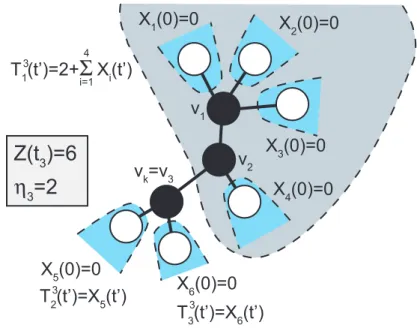
LetTk= inf{t:n(t) =k}represent the time whenkthnode is infected. It can be easily checked that for d≥3regular tree with exponential spreading time distribution,Tk<∞with probability1. Considert≥Tk. Fork≥2, letvkbe thekthinfected node when the rumor starts fromv
1. We will evaluate the probability of
identifyingvkas the rumor center. LetGrepresent the rumor infected tree observed at timetwithn(t)≥k nodes. Letw1, . . . , wdbe thedneighbors ofvk, as is illustrated in Figure 5. We shall denote the neighbor of
vk that is along the path joiningvkandv1asw1. Note thatw1must have been infected beforevk when the
rumor starts spreading fromv1. Letw2, . . . , wdbe thed−1‘children’ ofvk, away fromv1.
For convenience, we shall use notationt0=t−Tkwitht0≥0. LetTk i (t
0)be the subtree ofGrooted atwi at timetaway fromvk. Therefore,Tk
1(t
0)is rooted atw
1 and includesv1, . . . , vk−1. For 2≤i≤d,Tik(t 0) are rooted atwiand contain nodes inGthat are away fromvk. None of theTk
i (t0)for1≤i≤dincludevk. Whenvk is infected at timeTk, we have thatTk
1(0) =k−1, andT
k
i (0) = 0for2≤i≤d. This notation is illustrated in Figure 5.
By definition Tk
1 (t
0) is never empty, but Tk i (t
0) can be empty ifwi is not infected, for 2≤i≤d. As before, letTk
i(t0) =|T k
i (t0)|. As per Lemma 1,vk is identified as a rumor center if and only if all of itsd subtrees are balanced, i.e.
2Tik(t 0)≤1 + d X j=1 Tjk(t 0), ∀1≤i≤d. (4.6)
Therefore, fort≥Tkwitht0=t−Tk,
PCk t ≥P∩d i=1Ei = 1−P∪d i=1E c i ≥1− d X i=1 PEc i , and (4.7)
P Ctk ≤P ∩d i=1Fi = 1−P ∪d i=1F c i =1− d X i=1 P Fic , (4.8) whereEi={2Tk i(t 0)<1 +Pd j=1T k j(t 0)}andFi={2Tk i(t 0)≤1 +Pd j=1T k j(t 0)}.
As before, we shall evaluate these probabilities by studying the evolution of the appropriate rumor bound-aries. However, unlike for k= 1, when k≥2 the rumor boundaries have asymmetric initial conditions. Specifically,Tk 1 (0) =k−1, Z k 1(·) = (d−2)(k−1) + 1 and for 2≤i≤d, T k i (0) = 0 andZ k i(0) = 1. Beyond this difference, the rules governing the evolution of the rumor boundaries are the same as those described in the proof fork= 1. To evaluateEc
1(andF
c
1), we consider a Polya’s urn in which we start with (d−2)(k−1) + 1balls of type1 (corresponding toZk
1(0)) andd−1 balls of type2(corresponding to
Pd
j=2Z
k
j(0)). With these initial conditions, the limit law of fraction of balls of type1turns out to be (see Athreya and Ney (1972) for details) a Beta distribution with parameters a= ((d−2)(k−1) + 1)/(d− 2) = (k−1) + 1/(d−2)andb= (d−1)/(d−2) = 1 + 1/(d−2). Finally, since the fraction of balls of type1, i.e. the ratioZk
1(t 0)/(Pk j=1Z k j(t 0)), equals Tk 1(t 0)/(1 +Pd j=1T k j(t 0))ast0→ ∞, we obtain lim t0→∞P Ec 1 = lim t0→∞P Fc 1 = 1−I1/2 k−1 + 1 d−2, 1 + 1 d−2 . (4.9)
For2≤i≤d, in the corresponding Polya’s urn model, we start with1ball of type1andk(d−2) + 1balls of type2. Therefore, using an identical sequence of arguments, we obtain that for2≤i≤d,
lim t0→∞P Ec i = lim t0→∞P Fc i = 1−I1/2 1 d−2, k+ 1 d−2 . (4.10)
From (4.7)-(4.10), it follows that
lim t→∞P Ck t =I1/2 k−1 + 1 d−2, 1 + 1 d−2 + (d−1)I1/2 1 d−2, k+ 1 d−2 −1. (4.11)
This establishes (3.2) for allkand completes the proof of Theorem 3.1.
4.2. Proof of Lemma 1
We provide here a proof of Lemma 1 for the convenience of the reader. Much of this proof is taken from Shah and Zaman (2010). We begin by establishing the following property about rumor centrality.
Proposition 1 Consider an undirected tree graphG= (V, E)with|V|=Nand any two neighboring nodes
u, v∈V such that(u, v)∈E. The rumor centralities of these two nodes satisfy the following relationship:
R(u, G) R(v, G) = Tv u N−Tv u . (4.12)
We now show that ifvis a rumor center then it must satisfy the condition given by equation (4.2) in Lemma 1. For any nodeineighboring the rumor centerv, Proposition 1 gives
R(i, G) R(v, G)= Tv i N−Tv i ≤1. Rearranging terms, we obtain
Tv i ≤ N 2 ≤ 1 2 1 + X j∈N(v) Tv j .
We now establish the other direction of Lemma 1. Assume equation (4.2) of the Lemma is satisfied for a nodev. We now show thatvmust be a rumor center.
Leti∈V be a nodedhops fromvand let{v0=v, v1, v2, ..., vd=i}be the sequence of nodes in the path
betweenvandi. Using Proposition 1 we obtain
R(i, G) R(v, G) = d Y i=1 R(vi, G) R(vi−1, G) = d Y i=1 Tvi−1 vi N−Tvi−1 vi . The subtrees on the path betweenvandihave the special property thatTvi−1
vi =Tvv
ifori= 1,2, ..., dbecause the nodes in the subtree rooted atvi are the same if the subtree is directed away fromvi−1orv. We also
have the property thatN/2≥Tv vi−1 > T
v
vi fori= 2, ..., dbecause the subtrees must decrease in size by at least one node as we traverse the path fromvtoiand nodev satisfies equation (4.2) in the Lemma. With these facts we obtain
R(i, G) R(v, G) = d Y i=1 Tv vi N−Tv vi ≤1. (4.13)
If the inequality is strict in equation (4.2), then we have that for anyi6=v,Tv
i < N/2. Using Proposition 1 it can be shown that this implies that for everyi6=v, there exists a nodej6=isuch thatTi
j > N/2. This violates equation (4.2), which meansicannot be a rumor center. Therefore,vis the unique rumor center.
4.3. Proof of Proposition 1
The rumor centrality of a nodevin a treeG= (V, E)with|V|=N is given by
R(v, G) =Q N!
w∈VTwv with the tree variablesTv
wdenoting the size of the subtree ofGthat is rooted atwand points away fromv. For any two nodesu, v in a tree such that(u, v)∈E there is a special relationship between their subtrees. For anyw∈V, w6=u, v, it can be shown that Tv
w=T u
w. Also, it can be shown thatT v
u contains all nodes which are not inTu
v . This gives the simple relation thatT u
v =N−T v
u. With these results on the subtree variables we obtain R(u, G) R(v, G) = Q w∈V T v w Q w∈V Tvw = T v u N−Tv u .
4.4. Proof of Corollary 1
Simple analysis yields Corollary 1. We start by defining the asymptotic probability for ad-regular tree as limt→∞P(Ct1) =αd. This quantity then becomes
αd=dI1/2 1 d−2,1 + 1 d−2 −d+ 1 =1− dΓ(1 + 2 d−2) Γ( 1 d−2)Γ(1 + 1 d−2) Z 1 1 2 td−12−1(1−t)d−12dt
We then take the limit asdapproaches infinity.
lim d→∞αd= limd→∞1− dΓ(1 + 2 d−2) Γ(d−12)Γ(1 +d−12) Z 1 1 2 td−12−1(1−t)d−12dt = 1− lim d→∞ dΓ(1 + 2 d−2) (d−2−γ+O(d−1)) Γ(1 + 1 d−2) Z 1 1 2 td−12−1(1−t) 1 d−2dt = 1− Z 1 1 2 t−1dt = 1−ln (2).
Above,γis the Euler-Mascheroni constant and we have used the following approximation ofΓ(x)for small x:Γ (x) =x−1−γ+O(x).
4.5. Proof of Corollary 2
Corollary 2 follows from (3.2) and monotonicity of theΓfunction over[1,∞). Fork≥2,
lim t→∞P Ctk =I1/2 k−1 + 1 d−2,1 + 1 d−2 + (d−1) I1/2 1 d−2, k+ 1 d−2 −1 ≤I1/2 k−1 + 1 d−2,1 + 1 d−2 = Γ(k+ 2 d−2) Γ(k−1 + 1 d−2)Γ(1 + 1 d−2) Z 12 0 tk+d−12−2(1−t) 1 d−2dt (a) ≤ Γ(k+ 2 d−2) Γ(k−1 +d−12)Γ(1 +d−12) Z 12 0 tk−2dt (b) ≤ 4e 2Γ(k+ 2) Γ(k−1) Z 12 0 tk−2dt (c) ≤4e2k(k+ 1)(k+ 2) 1 2 k−1 exp −Θ(k) .
In above, (a) follows from the fact thatt <1and hencetk−2+1/(d−2)≤tk−2. For (b), we use the following
well-known properties of theΓ function: (i) over [2,∞), theΓ function is non-decreasing and hence for k≥2andd≥3,Γ(k+(d−22))≤Γ(k+ 2); (ii) over(0,∞), theΓfunction achieves its minimal value in[1,2] which is at least 1
2eand therefore, along with (i), we have thatΓ(k−1 +
1 d−2)≥ Γ(k−1) 2e andΓ(1 + 1 d−2)≥ 1 2e. For (c), we use the fact thatΓ(x+ 1) =xΓ(x)for anyx∈(0,∞).
4.6. Proof of Theorem 3.2: Correct Detection for Random Trees
The goal is to establish that there is a strictly positive probability of detecting the source correctly as the rumor center when the rumor starts at the root of a generic random tree with generic spreading time dis-tribution as defined earlier. The probability is with respect to the joint disdis-tribution induced by the tree construction and the SI rumor spreading model with independent spreading times. We extend the tech-nique employed in the proof of Theorem 3.1. However, it requires using a generalized Polya’s urn or age-dependent branching process as well as delicate technical arguments.
4.6.1. Background: Age-Dependent Branching Process. We recall a generalization of the classical Polya’s urn known as an age-dependent branching process. Such a process starts at timet= 0with a given finite number of nodes, sayB(0)≥1. Each node remains alive for an independent, identically distributed lifetime with cumulative distribution function given byF: [0,∞)→[0,1]. The lifetime distribution func-tionF will be assumed to be non-atomic at0, i.e.F(0+) = 0. Each node dies after remaining alive for its
lifetime. Upon the death of a node, it gives birth to random number of nodes, sayη. The random variablesη corresponding to each node are independent and identically distributed over the non-negative integers. The newly born nodes live for their lifetime and the upon death give birth to new nodes, and so on.
As can be seen, the classical Galton-Watson process is a special case of this general model and the size of the entire urn in the Polya’s urn process described earlier naturally fits this model. An interested reader is referred to Athreya and Ney (1972) for a detailed exposition. Next we recall certain remarkable asymptotic properties of this process that will be crucially utilized. We start with a useful definition.
Definition 4 (Athreya and Ney 1972, pp. 146) Letm≡E[η]. The Malthusian parameterα=α(m, F)of an age-dependent branching process is the unique solution, if it exists, of the equation
m
Z ∞
0
e−αydF(y) = 1. (4.14)
A sufficient condition for the existence of the Malthusian parameter is m=E[η]>1. As an example,
consider process where spreading time distribution is exponential with parameterλ, i.e.F(t) = 1−e−λt, and letm=E[η]>1. The Malthusian parameterα(m, F)is given by the solution of
m
Z ∞
0
which is
α(m, F) =λ(m−1).
The Malthusian parameter captures the average growth rate of the branching process. We now recall the following result.
Theorem 4.2 (Athreya and Ney 1972, Theorem 2, pp. 172) Consider an age-dependent branching process as described above with the additional properties thatm=E[η]>1andE[ηlogη]<∞. Letα≡α(m, F)
be the Malthusian parameter of the process and define
c= m−1 αm2R∞
0 ye
−αydF(y).
LetB(t)denote the number of nodes alive in the process at timet≥0. Then
1 ceαtB(t)
t→∞
→ W in distribution,
whereW is such that
E[W] = 1 (4.15) P W= 0 =q, (4.16) P W∈(x1, x2) = Z x2 x1 w(y)dy, for 0< x1< x2<∞, (4.17)
whereq∈(0,1)is the smallest root of the equationP∞
k=0s
kP(η=k) =sandw(·)is absolutely continuous
with respect to the Lebesgue measure so thatR0∞w(y)dy= 1−q.
The above result states that with probabilityq(0< q <1) the branching process becomes extinct, and with probability 1−q the size of the process scales as exp(αt)for large t. We will need finer control on the asymptotic growth of the branching process. Precisely, we shall use the following implication of the above stated result.
Corollary 3 Under the setting of Theorem 4.2, for anyf >1, there exists anx >0so that P W∈(x, f x)
>0. (4.18)
ProofDefine
ak=fk, for k∈
By definition, {W >0}=∪k∈Z {W∈(ak, ak+1]}. Due to the absolute continuity of w(·) in (4.17), it
follows thatP(W=ak) = 0for allk∈Z. Therefore, it follows that
0<P W >0 =P ∪k∈Z W∈(ak, ak+1) ≤X k∈Z P W∈(ak, ak+1 . (4.19)
From above, it follows that there exists aksuch thatP W∈(ak, ak+1)
>0. This completes the proof.
4.6.2. Notation. We quickly recall some notation. To start with, as before letv1be the root node of the
tree. It hasη0 children distributed as perD0. Define the event A={η0≥3}. By assumption of Theorem
3.2,P(A)>0. We shall show that
lim inf t→∞ P(C
1
t|A)>0, (4.20)
as it will imply the desired resultlim inft→∞P(Ct1)>0, usingP(A)>0sinceP(C
1
t)≥P(C
1
t|A)P(A). Therefore, we shall consider conditioning on eventAand letd=η0≥3for remainder of the proof. Note that
all the spreading times as well as all other randomness are independent ofη0. The only effect of conditioning
onAis that we know that root hasd≥3children. Letu1, . . . , ud be thedchildren of rootv1. The random
treeGis constructed by adding a random number of children tou1, . . . , udrecursively as per distributionD
as explained in Section 3.2.
Further, as explained in Section 3.2, the rumor spreads onGstarting fromv1at time0as per the spreading
times with cumulative distribution function F that is non-atomic at0. Let G be the sub-tree ofG that is infected at timetwithn(t)infected nodes inGat timet. LetTi(t)denote the subtree ofGrooted at node ui (pointing away from rootv1) at timet, for1≤i≤dand letTi(t) =|Ti(t)|. By definitionTi(0) = 0for 1≤i≤d. LetZi(t)denote the size of the rumor boundary ofTi(t); initiallyZi(0) = 1, 1≤i≤d.
Now let us consider the evolution of Zi(·): recall that each node in the rumor boundary has a rumor infected parent (neighbor). This node will become infected after the amount of time given by the spreading time associated with the edge connecting the node with its infected parent. After the node becomes infected, it is no longer part of the rumor boundary, but all of its uninfected neighbors (children) become part of the rumor boundary. And as per the random generative process of the tree construction, the number of children added,η, has distributionD. Therefore, the rumor boundary processZi(·)for each1≤i≤dis exactly an age-dependent branching process. Further, eachZi(·)evolves independently and since initially each starts at the same time with exactly one node, they are identically distributed. Therefore, we can utilize the results stated in Section 4.6.1 to characterize the properties ofZi(·)for1≤i≤d. In the case of regular trees,Zi(·) andTi(·) were linearly related which allowed us to obtain results aboutTi(·)and the desired conclusion. While in this general setting,Zi(·)andTi(·)are not linearly related, we show that they are asymptotically linearly related due to an appropriate Law of Large Numbers effect. This will help us obtain the desired conclusion. We present the details next.
4.6.3. Correct Detection. As before, we wish to show that P Ct1|A ≥P ∩d i=1 n 2Ti(t)<1 + d X j=1 Tj(t) o , (4.21)
where we have removed the conditioning onA, as the only effect ofAwas havingddistinct trees, which is already captured. We shall establish (4.21) in two steps:
Step 1. Using the characterizations of Zi(·) in terms of age dependent branching processes as dis-cussed above, we shall show that there is a non-trivial event E1 ⊂ ∩di=1
n 2Zi(t) <Pd j=1Zj(t) o with lim inft→∞P(E1)>0.
Step 2.Identify an eventE2⊂ E1withlim inft→∞P(E2)>0andE2⊂ ∩di=1
n
2Ti(t)<1 +Pd
j=1Tj(t)
o
for alltlarge enough.
This will yield the desired results.
4.6.4. Step 1. For anyx >0andε >0define the eventE(x, ε, t)as
E(x, ε, t) =∩d i=1
n
Zi(t)c−1e−αt∈(x,(1−3ε)(d−1)x)o. (4.22)
Sinced≥3,(1−3ε)(d−1)>1for small enoughε >0and hence the above event is well defined. It can be easily checked thatE(x, ε, t)⊂ ∩d
i=1
n
2Zi(t)<Pd
j=1Zj(t)
o
, since under this event,
max
i Zi(t)≤(1−3ε)(d−1)x <(d−1)x≤(d−1) mini Zi(t).
By Theorem 4.2, it follows thatZi(t)c−1e−αt converges toWi, which are independent acrossiand iden-tically distributed as per (4.16)-(4.17). Therefore, using Corollary 3, it follows that there exists anx∗>0 such that lim inf t→∞ P E(x∗, ε, t)>0. (4.23) DefineE1=E(x∗, ε, t).
4.6.5. Step 2. We want to findE2⊂ E1so that fortlarge enough,E2⊂ ∩di=1
n
2Ti(t)<1 +Pd
j=1Tj(t)
o
andlim inft→∞P(E2)>0. For regular trees this was achieved by using the linear (deterministic)
relation-ship between theZi(·) andTi(·). Here, we do not have such a relationship. Instead, we shall establish an asymptotic relationship. To that end, recall that for anyt≥0,
Zi(t) = 1 + X `∈Ti(t)
(η`−1). (4.24)
The above holds because as per the branching process, when a node in the ‘boundary’ dies (−1is added to Zi(·)) and it is added toTi(·),η`new nodes are added to boundary.
ConsiderTi(·). It grows by adding nodes with a random number of children as per distributionD inde-pendently. Let η1, η2, . . . be these random number of children added to it in that order (we assume this
sequence to be infinite irrespective of whether or not Ti(·) stops growing). Since these are i.i.d. random variables with finite mean (actually,E[ηlogη]<∞), by the standard Strong Law of Large Numbers, for any small enoughε, δ >0, with probability at least1−δ, for all1≤i≤d, we have that for allp≥1
(1−ε)p
m −C(ε, δ)≤Ni(p) ≤
(1 +ε)p
m +C(ε, δ) (4.25)
where Ni(p) = inf{`:P`
j=1(ηj −1)≥p},m=E[η]and C(ε, δ) is a non-negative constant depending
uponε, δ but independent ofp. Let us call the event represented by (4.25) as E0(ε, δ). Here, we have the freedom of choosing as small a δ andεas we like. We will chooseδ so that it is much smaller than the probability of eventE1 fortlarge enough. Given such a choice, it will follow that for all tlarge enough,
the eventE2=E1∩ E0(ε, δ) has strictly positive probability. Under eventE2, we have (with the definition ˆ Zi(t) =Zi(t)c−1e−αt) ˆ Zi(t)∈(x∗, x∗(1−3ε)(d−1)), for all 1≤i≤d, (4.26) Ti(t)c−1e−αt∈ Ziˆ(t)(1−ε) m −at, ˆ Zi(t)(1 +ε) m +at ! for all1≤i≤d,
where the constants at→0 ast→ ∞. Therefore, it can be easily checked that for tlarge enough andε small enough, E2⊂ ∩di=1
n
2Ti(t)<1 +Pd
j=1Tj(t)
o
, just the way we argued that E1⊂ ∩di=1
n
2Zi(t)<
Pd
j=1Zj(t)
o
. As discussed above, with an appropriate choice of δ and ε, we can guarantee that lim inft→∞P(E2)>0. This concludes the search for the desired event E2 and we have established the
desired claim oflim inft→∞P(Ct1)>0. This completes the proof of Theorem 3.2.
4.7. Proof of Theorem 3.3
4.7.1. Background: Properties of Age-Dependent Branching Processes. We shall utilize the follow-ing property known in the literature about bounds on the moment generatfollow-ing function of the size of an age-dependent branching process. We shall assume the notation from the earlier section.
Theorem 4.3 (Nakayama et al. 2004, Theorem 3.1) Consider an age dependent branching process with the properties thatm=E[η]>1,E[exp(θη)]<∞for allθ∈(0, θ1)for someθ1>0, and the spreading time
distribution is non-atomic. LetB(t)represent the number of living nodes in the branching process at timet
and letV(t)represent the number of nodes born before timet. Then, there exists aθ∗>0such that for all
θ∈(−θ∗, θ∗) E eθB(t) ≤E eθV(t) <∞. (4.27)
4.7.2. Background: Two inequalities. We state two useful concentration-style inequalities that we shall derive here for completeness.
Proposition 2 For i≥1 let Xi be independent and identically distributed random variables such that E[exp(θX1)] < ∞ for all θ ∈ (−δ, δ) for some δ > 0. Then, for any ε > 0, there exists constants
C1, C2(ε, δ)>0such that P n X i=1 Xi≤µn(1−ε) ! ≤C1exp −C2(ε, δ)µn , (4.28) whereµ=E[X1].
Proposition 3 Consider independent and identical random variablesX1, . . . , Xr+sfor integersr, s such
that1≤s < r. Letµ=E[X1]andE[exp(θX1)]<∞for allθ∈(−δ, δ)for someδ >0. Then there exists
a constantcsuch that for anyγ >0, there exists a constantθ∗= min(γ+(r−s)µ
2(r+s)c , δ1/2)for some0< δ1< δ, such that P( r X i=1 Xi− s X j=1 Xr+j≤ −γ)≤exp − 1 2θ ∗(γ+ (r−s)µ) . (4.29)
Next, we prove these two propositions.
Proof of Proposition 2. LetX be a random variable with identical distribution as that ofXi, i≥1. By assumption in the Proposition statement, it follows that forθ∈(−δ, δ)
MX(θ)≡logE[exp(θX)] = log 1 + ∞ X j=1 θjE[Xj]/j! ≤log1 +θµ+cθ2,
for somec >0for allθ∈(−δ1, δ1)for some0< δ1< δ. Using the inequalitylog(1 +x)≤xfor allx >−1,
we obtain
MX(θ)≤θµ+cθ2. (4.30)
Now, for anyΓ>0andθ >0, using standard arguments and (4.30), we obtain
P( n X i=1 Xi≤nµ−Γ) =P exp(−θ( n X i=1 Xi−nµ))≥exp(Γθ) ≤exp(−θΓ +θnµ)E[exp(−θX)]n = exp −θΓ +θnµ+nMX(−θ) ≤exp −θΓ +cnθ2 (4.31)
For any0< θ≤Γ/(2nc), P( n X i=1 Xi≤nµ−Γ)≤exp −1 2Γθ . UsingΓ =nµεandθ∗= min(δ/2, µε/(2c)), we have
P( n X i=1 Xi≤nµ(1−ε))≤exp −1 2nµεθ ∗ = exp −C2(ε, δ)nµ , (4.32)
whereC2(ε, δ) =12εmin(δ/2, µε/(2c)). This completes the proof of Proposition 2.
Proof of Proposition 3.Given1≤s < r,γ >0andθ >0, using standard arguments (with the notation that the random variableXhas an identical distribution asXi,1≤i≤r+s)
P( r X i=1 Xi− s X j=1 Xr+j≤ −γ) =P(−θ( r X i=1 Xi− s X j=1 Xr+j)≥γθ)
≤exp(−θγ)E[exp(−θX)]rE[exp(θX)]s.
Using notation and arguments similar to that in the proof of Proposition 2, we conclude that the above inequality can be bounded above, for somec >0andθ∈(−δ1, δ1)for0< δ1< δas
P( r X i=1 Xi− s X j=1 Xr+j≤ −γ)≤exp(−θγ+ (s−r)θµ+ (r+s)cθ2). (4.33)
Forθ∗= min(γ2(+(rr+−ss))cµ, δ1/2), we obtain
P( r X i=1 Xi− s X j=1 Xr+j≤ −γ)≤exp − 1 2θ ∗(γ+ (r−s)µ) . (4.34)
4.7.3. Proof of Theorem 3.3. Theorem 3.3 assumes that the spreading times have an exponential dis-tribution with (unknown) parameterλ >0for all edges. The underlying graph is a generic random tree, just like that in Theorem 3.2. We shall crucially utilize the ‘memory-less’ property of the exponential distribu-tion to obtain the exponential error bound onlim supt→∞P(Ck
t)claimed in Theorem 3.3.
To that end, continuing with notations from the proof of Theorem 3.2, letTk= inf{t >0 :T(t) =k}. By definition, lim sup t→∞ P(Ctk|Tk=∞) = 0. (4.35) Therefore, lim sup t→∞ P(Ck t)≤lim sup t→∞ P(Ck t|Tk<∞). (4.36)
Therefore, let us assume thatTk<∞and we will be interested int > Tk. We shall re-define the index for time ast0 =t−Tk. When t0 = 0, we have exactly k nodes infected and let them be v
1, . . . , vk,
v
1v
k=v
3X
1(0)=0
v
2X
2(0)=0
X
6(0)=0
X
4(0)=0
X
3(0)=0
X
5(0)=0
Z(t
3)=6
η
3=2
T
23(t’)=X
5(t’)
T
33(t’)=X
6(t’)
T
13(t’)=2+
Σ
X
i(t’)
i=1 4Figure 6 Illustration of the labeling of the subtree random processesXj(t0)fork= 3in a rumor graph att=tk(the time of infection ofvk). The rumor infected nodes are colored black, and the uninfected nodes are white.
the neighbor ofvk on the path connecting vk andv1 and letw2, . . . , wd be the other neighbors of vk. Let Tk
1(t0)(withT
k
1(t0) =|T
k
1(t0)|) be the sub-tree rooted atw1includingv1(and not includingvk). Similarly,
letTk
j (t0)(withT k
j(t0) =|T k
j (t0)|) be the sub-tree rooted atwj,