Bard College Bard College
Bard Digital Commons
Bard Digital Commons
Senior Projects Spring 2017 Bard Undergraduate Senior Projects Spring 2017
Community Detection for Counter-Terrorism
Community Detection for Counter-Terrorism
Patrick Michael Kelly
Bard College, [email protected]
Follow this and additional works at: https://digitalcommons.bard.edu/senproj_s2017
Part of the Numerical Analysis and Scientific Computing Commons
This work is licensed under a Creative Commons Attribution-Noncommercial-No Derivative Works 4.0 License. Recommended Citation
Recommended Citation
Kelly, Patrick Michael, "Community Detection for Counter-Terrorism" (2017). Senior Projects Spring 2017. 361.
https://digitalcommons.bard.edu/senproj_s2017/361
This Open Access work is protected by copyright and/or related rights. It has been provided to you by Bard College's Stevenson Library with permission from the rights-holder(s). You are free to use this work in any way that is permitted by the copyright and related rights. For other uses you need to obtain permission from the rights-holder(s) directly, unless additional rights are indicated by a Creative Commons license in the record and/or on the work itself. For more information, please contact
Community Detection for Counter-Terrorism
A Senior Project submitted to The Division of Science, Mathematics,
and Computing of Bard College
By Patrick Kelly
Annandale-on-Hudson, New York
Abstract
Community detection in large networks is a process that has been heavily researched in the past decade due to the the emergence of online social networks. For Twitter, Inc., analyzing terrorists communities is vital in the fight against ISIS recruiters who use the twitter platform to radicalize people around the world. The goal of this project is to develop an algorithm which can accurately detect communities in large networks and to provide textual analysis on the discovered communities. Our algorithm combines the results of two unsupervised clustering algorithms to find communities in a given network. One algorithm uses the structure of the network, and the other algorithm uses the text associated with the nodes. Our algorithm is tested on a hand labeled ground truth twitter network and applied to an ISIS twitter recruiting network.
Acknowledgements
I would like to thank...
• My parents for supporting me through everything.
• Professor Sven Anderson and Professor Khondaker Salehin for pushing me each week and advising my research with unending positive energy.
• My friends and teammates for the great times we’ve had together.
• Coach Adam Turner for helping me become better on and off the court.
Dedication
I dedicate this project to Alexei Phillips ’06.
Contents
Abstract i Acknowledgements iii 1 Introduction 1 1.1 Background . . . 1 1.2 Network Science . . . 3 1.3 Clique Percolation . . . 4 1.4 TF and TF-IDF . . . 51.5 Non-negative Matrix Factorization . . . 6
1.6 Set Theory . . . 7
1.7 Choosing K . . . 7
1.8 Latent Dirichlet Allocation . . . 9
1.9 The Big-Clam . . . 10
1.10 K-Means Textual Clustering with PCA . . . 10
1.11 Past Research . . . 11 vii
viii CONTENTS 2 Methods 12 2.1 Overview . . . 12 2.2 Clique Percolation . . . 12 2.3 NMF on the Text . . . 13 2.4 Set Comparisons . . . 14 2.5 Topic Extraction . . . 14
2.6 Evaluation on Ground Truth . . . 15
3 Results 16 3.1 The Ground Truth Data Set . . . 16
3.2 The Bard Community . . . 18
3.3 The Massachusetts Community . . . 20
3.4 The Athletics Community . . . 22
3.5 The Music Community . . . 24
3.6 The Family Community . . . 26
3.7 The Politics Community . . . 28
3.8 The Basketball Community . . . 29
3.9 The Computer Science Community . . . 30
3.10 Failure of BigClam and K-means . . . 31
3.11 Average F1 Scores by Algorithm . . . 33
4 Conclusion 35
4.1 Summary of Thesis Achievements . . . 35
4.2 Applications . . . 35
4.3 Future Work . . . 36
Bibliography 36 A The BigClam Python Implementation 39 B Generating a Ground Truth Data Set From Twitter 43 B.1 getFollowers.py . . . 43
B.2 getTheTweets.py . . . 43
B.3 buildNetwork.py . . . 44
B.4 twitterNetwork.py . . . 47
List of Figures
1.1 The ISIS Twitter Recruiting Network. . . 2
1.2 Probabilistic Model of LDA [1]. . . 9
3.1 The Ground Truth Network. . . 17
3.2 Bard Clique Percolation Results with F1 Score: 0.948905109489. . . 18
3.3 Bard NMF Results with F1 Score: 0.476987447699. . . 18
3.4 Bard Combination Results with F1 Score: 0.501766784452. . . 19
3.5 Massachusetts Clique Percolation Results with F1 Score: 0.786206896552. . . 20
3.6 Massachusetts NMF Results with F1 Score: 0.271428571429. . . 20
3.7 Massachusetts Combination Results with F1 Score: 0.524390243902. . . 21
3.8 Athletics NMF Results with F1 Score: .371428571429. . . 22
3.9 Athletics Combination Results with F1 Score: 0.225563909774. . . 23
3.10 Music Clique Percolation Results with F1 Score: 0. . . 24
3.11 Music NMF Results with F1 Score: .29219325239. . . 24
3.12 Music Combination Results with F1 Score: .201293491293. . . 25
3.13 Family Cliaue Percolation Results with F1 Score: 0.615384615385. . . 26 xi
3.14 Family NMF Results with F1 Score: 0.0769230769231. . . 26
3.15 Family Combination Results with F1 Score: 0.585384615385. . . 27
3.16 Politics Clique Percolation Results with F1 Score: 0. . . 28
3.17 Politics NMF Results with F1 Score: 0.124031007752. . . 28
3.18 Basketball NMF Results with F1 Score: 0.410109209349. . . 29
3.19 Basketball Combination Results with F1 Score: 0.310344827586. . . 30
3.20 Computer Science Combination Results with F1 Score: 0.310344827586. . . 31
3.21 BigClam Bard Community Results with F1 Score: .461929432. . . 32
Chapter 1
Introduction
1.1
Background
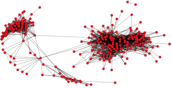
This community detection algorithm utilizes concepts from the areas of network science and text analysis. The algorithm was inspired by the ISIS Twitter Recruiting data set (kaggle.com). The data set features 17,000 tweets by 112 ISIS recruiters from 2014-2016. There has been significant research in both network science and text analysis on the topic of clustering within each field independently, however, effectively combining methods from both fields has not yet been explored to a significant degree. The CESNA algorithm [7] uses network attributes to cluster sets of nodes into communities where nodes can be associated with multiple communities. First, it is important to acknowledge that nodes in communities share properties and have many relationships amongst themselves which are independent of their network structures. This is key to understanding that there are multiple sources of data which can be used to perform the clustering task. In our case, we have a network with text data(tweets) associated with the nodes. This means that our input data is more complex than the input data necessary to run CESNA.
In this paper, we considertrue communitiesto be groups of people that share interests or live in the same area. The algorithm that we build is a community detection algorithm, but it is important distinguish the types of communities we strive to discover are different than
2 Chapter 1. Introduction
what typical community detection algorithms search for. While many researchers have defined “communities” as groups of densely connected nodes, this is only a part of detecting “true” communities as we define them.
The network is constructed by assigning each user to a node and each tweet @ another recruiter as an edge. Take for example the following tweet written by the recruiter named @ISBAQIYA “@spamci16: More than 70000 childrens have been killed by Assad regime. Why cry only for the drowned child? Hypocricy of the world.” This tweet would lead to the construction of an edge between @ISBAQIYA and @spamci16. When analyzing the text, all tweets from one user are appended together and treated as one document. The following sections feature brief explanations of the theory behind each step of our algorithm which utilizes both the network structure and the text data to group the users into communities.
1.2. Network Science 3
1.2
Network Science
Network Science is the study of systems using their network structure or topology. A net-work’s structure can be described by a bunch of nodes and edges between pairs of nodes that represent a connection of some sort. In the case of the ISIS twitter recruiting data set, the recruiters themselves are represented by nodes and the social interactions between the users are represented as edges.
A directed network is a network that contains only edges that can only run in one direction. We build an undirected network, which is a network that contains edges that point in both directions which represents a simple connection between nodes[8]. An undirected network is utilized because much more research has been produced in community detection algorithms in undirected networks.
A network can be represented as a square matrix. A matrix that corresponds to a given network is called it’s adjacency matrix. The rows and columns are represented by the nodes in the network, with a 1 or 0 in position (vi, vj). If vi is adjacent to vj than position (vi, vj)
is represented by a 1. If vi is not adjacent to vj than position (vi, vj) is represented by a 0.
We take an undirected network, and the resulting adjacency matrix is symmetric. A weighted network can be represented in an adjacency matrix by assigning values that correspond to the weights of the connections [10].
There are a few key terms to understand that are used to describe characteristics of networks. The degree of a node in a network is the number of edges connected to it. The path is any sequence of nodes such that every consecutive pair of nodes in the sequence is connected by an edge in the network. A path’s length is described by the number of edges traversed along the path. The geodesic path is the shortest path between any two nodes. The centrality
of a node is a measurement of the node’s importance in the network. The most simple way of measuring centrality is the degree. The higher the degree, the more central the node is to the network. But as networks grow larger and have higher complexity, it’s easy to see that degree is not always the best way to define centrality. A more complex measurement of centrality is
4 Chapter 1. Introduction
closeness centrality. Closeness is a measure of the degree to which an individual is near all other individuals in a network. It is the inverse of the sum of the shortest distances between each node and every other node in the network. Another method, called betweenness centrality, is a measure of the extent to which a node is connected to other nodes that are not connected to each other. Its essentially a measure of the degree to which a node serves as a bridge [10].
Numerous methods have been developed over the years in order to analyze networks based off of their structure. The development of online social networks like Facebook and Twitter led to a heightened interest in grouping network nodes into communities. Communities are found in networks that have tightly knit groups of nodes with many edges between them with looser connections outside of the communities. Community structure stemmed from the concepts of network clustering. Clustering is based off of a concept known as network transitivity, which is a postulate which states that two nodes that are both neighbors of the same third node have a heightened probability of also being neighbors of one another.
As research has progressed, three major categories of community detection algorithms have emerged: hierarchical, optimization, and others. We implement Clique Percolation due to it’s inherent ability to detect overlapping communities. Clique Percolation is considered a member of the “other” category in the greater score of community detection algorithms. Clique Percolation utilizes network structure and probability concepts to group nodes in a graph into communities.
1.3
Clique Percolation
Clique Percolation is an effective algorithm for detecting overlapping communities in large graphs. Before the creation of the Clique Percolation clustering algorithm, most techniques used to find communities in large networks required the division of networks into smaller con-nected clusters by the removal of key edges which connect dense sub-graphs. This process is not effective for discovering overlapping networks because the removed edges could be key in detecting a different community later in the process.
1.4. TF and TF-IDF 5
The following definitions are important for understanding the clique percolation algorithm.
Cliques are fully connected sub-graphs of k vertices. K-clique adjacency means two k-cliques are adjacent if they share k1 vertices. A k-clique chain is a sub-graph which is the union of a sequence of adjacent k-cliques. Two k-cliques are k-clique-connected if they are parts of a k-clique chain. A k-clique percolation cluster (or component): is a maximal k-clique-connected sub-graph, meaning it is the union of all k-cliques that are k-k-clique-connected to a particular k-clique.
The algorithm finds k-cliques, which correspond to fully connected sub-graphs of k nodes. It understands a community as the maximal union of k-cliques that can be reached from each other through a series of adjacent k-cliques. First, all of the existent maximal k-clique percolation clusters for the given k are discovered. The k-clique percolation cluster is a maximal k-clique-connected sub-graph. This is understood as the union of all k-cliques that are k-clique-k-clique-connected to a particular k-clique. The percolation transition takes place when the probability of two vertices being connected by an edge reaches the threshold pc(k) = [(k − 1)N]−1/(k−1) It is
proven in [3] that the success in overlapping community detection with clique percolation on randomized networks translates to success on real networks. This is because only small clusters would be expected for any k at which the networks is below the transition point, but large clusters do appear, they must correspond to locally dense structures.
1.4
TF and TF-IDF
While analyzing the network structure is an effective approach to discover communities in the ISIS twitter recruiting data, text clustering is another logical approach. Treating all tweets by a given user as a personal document, TF and TF-IDF are useful methods to vectorize the tweets associated with each recruiter.
Term frequency (TF) is a simple way of vectorizing text where all words in the corpus are featured in a vector for each document, and the frequency of each term is reflected in the number representing the corresponding word. The problem with TF is that there are many
6 Chapter 1. Introduction
words that may be used many times but are not helpful in clustering. TF-IDF is usually favored over TF for this reason.
TF-IDF is the term frequency-inverse document frequency. The result of calculating the TF-IDF for each word in a document is a vector of weights, with the importance of a term in its contextual document corpus represented by the weight. First, the term frequency is calculated as normalized frequency, which is the ratio of the number of occurrences of a word in its document to the total number of words in its document. To calculate the inverse document frequency, the logarithm of the ratio of the number of documents in the corpus to the number of documents containing the given term is calculated. This inversion assigns a higher weight to terms that are rare. Multiplying the TF and IDF gives the TF-IDF which values terms that are frequent to a particular user, but rare in the corpus. The TF-IDF weighting scheme assigns to term t a weight in documentd given bytf −idft,d =tft,d×idft With the standard
vector space model, a set of documents S can be expressed as a m×n matrix V, where m is the number of terms in the dictionary and n is the number of documents in S. Each column Vj of V is an encoding of a document in S and each entry Vij of vector Vj is the significance
of term i with respect to the semantics of Vj, where i ranges across the terms in the dictionary
[4]. With the important words for each document highlighted by TF-IDF we test multiple clustering techniques on the vectorized text data.
1.5
Non-negative Matrix Factorization
In Non-negative Matrix Factorization (NMF), a matrix V is factorized into two W and H where all of the elements are non-negative. In terms of text clustering, the size of V would be (number of words) by (number of documents). NMF requires an expected number to be given and this number is the number of features that it should find. The features matrix W would be of size (number of words) by (number of features). The coefficients matrix would become (number of features) by (number of documents). The product of W and H is a matrix of the same size as the input matrixV and is a fairly reasonable approximation of the input matrixV.
1.6. Set Theory 7
Each column in the resulting matrix from W H is a linear combination of the column vectors in the features matrix W with coefficients supplied by the coefficients matrixH. NMF for text clustering could be summed up as an extraction of latent features from high-dimensional data.
NMF’s power is in it’s ability to look at complex data and find hidden patterns. It finds a decomposition of samples X into two matricesW andHof non-negative elements, by optimizing for the squared Frobenius norm (we choose Frobenius norm because it is available in open source): arg min
W,H 1 2||X−W H||= 1 2 P i,j(Xij −W Hij) 2 [12].
It has been observed by many that NMF can produce a parts-based representation of the data set, resulting in interpretable models.
1.6
Set Theory
In order to utilize both the network structure and text associated with the nodes, we take concepts from set theory to combine the results of two clustered data types. These definitions are useful for understanding the steps taken in the process of algorithm combination. The
union of A and B is the set of all objects that are a member of A, or B, or both. The
intersection of the sets A and B is the set of all objects that are members of both A and B. The set differenceof U and A is the set of all members of U that are not members of A. The
symmetric difference of sets A and B is the set of all objects that are a member of exactly one of A and B (elements which are in one of the sets, but not in both). These definitions will help in our set matching for both combining the results of the two algorithms and for comparing to ground truth communities.
1.7
Choosing K
Choosing the amount of clusters to search for is a challenging problem faced by anyone dealing with clustering. K is the number representative of whatever is being searched for. In clique
8 Chapter 1. Introduction
percolation, k represents the size of the cliques that the algorithm discovers for. In NMF, k is the the number of features to be found.
For Cliaue Percolation, we set k = 3 on the test data and the ground truth data. In our ground truth data set, this produces a communities of sizes that make sense for the size of the data set. With k<3, there are too many small communities. With k>3, there are too few communities. Because the ISIS data set is of similar size and structure, we assume that 3 also produces communities with sizes that make logical sense.
For NMF, we utilize the NMF silhouette method to determine the optimal number of clusters. The silhouette score for a user gives us a measure of how closely matched it is to data within it’s cluster and how loosely it is matched to data of the neighbouring cluster. We choose the number of features in NMF which maximize the average silhouette score of the entire network. The following equations represent how the silhouette score for a single user s(i) is calculated.
s(i) =
1−a(i)/b(i), if a(i)<b(i)
0, if a(i) = b(i)
b(i)/a(i)−1, if a(i)>b(i)
s(i) = b(i)−a(i) max(a(i), b(i))
In general, a very large average silhouette width can be taken to mean that the clustering al-gorithm has discovered a very strong clustering structure. [11] However, if the data set contains multiple outliers, non-outliers may appear to be tighter than they actually are. Visualizing the data and removing clear outliers would be an effective step to aid the silhouette scoring method.
1.8. Latent Dirichlet Allocation 9
1.8
Latent Dirichlet Allocation
To provide information on the discovered communities, we utilize Latent Dirchlet Allocation (LDA). LDA can automatically discover topics in a corpus of documents by learning the topic representation of each document and the words associated to each topic. We utilize LDA in an unconventional way by using it only for it’s ability to find words associated with 1 topic. We know that our algorithm outperforms LDA in clustering the users, and we use LDA only to find words associated with the clusters that have already been discovered. By setting K equal to 1 and only searching through the users for one community, we find associated words for each community.
The idea is that documents are represented as random mixtures over latent topics, where each topic is characterized by a distribution over words. Figure 1.2 represents LDA as a probabilistic generative model and emphasizes the three levels of LDA.α andβ are sampled once while gen-erating the corpus. They are considered corpus-level parameters which feed the document-level variables θ. For each word, zdn and wdn sample once in the end of the process [1]. This bag of
words approach returns a list of words that are representative of each topic. We utilize the list of representative words to attempt to understand each detected community.
10 Chapter 1. Introduction
1.9
The Big-Clam
The BigClam algorithm utilizes the underlying adjacency matrix of the given graph to maximize the likelihood of a new matrix F which represents how strongly associated each node is with each community. BigClam formulates community detection as a variant of non-negative matrix factorization. Similar to NMF, BigClam aims to learn factors that can recover the adjacency matrix of a given network. Bloch coordinate gradient descent is used to solve the convex optimization problem of updating eachFu in the matrixF [6]. The original Big-Clam algorithm
utilizes shortcuts to lessen it’s computational cost, we created a python implementation without shortcuts because our data sets have edge lists with lengths in the thousands rather than the millions. The BigClam algorithm is unable to accurately detect communities in our ground truth data set. It’s impossible to point out exactly why the algorithm could not perform on our ground truth network. We do know that the authors construct their model under the following assumption: “On average 95 percent of all communities overlap with at least one other community and only 15 percent of communitys members belong to only that community. We thus examine the structure of community overlaps by measuring the probability of a pair of nodes being connected given that they belong to k common communities. [6] ” In our ground truth community, far less than 95 percent of communities overlap with at least one community. This may have been a reason for why the model misclassified most of the nodes.
1.10
K-Means Textual Clustering with PCA
Conducting K-Means clustering on high dimensional TF-IDF data requires some kind of di-mensionality reduction. We use principal component analysis (PCA) to reduce the text data’s dimensionality to 2 dimensions. PCA performs a linear mapping of the data by maximizing the variance of the data in the low-dimensional representation. The eigen-vectors on the matrix are computed and those that correspond to the largest eigenvalues can now be used to reconstruct a large fraction of the variance of the original data. The goal is to retain the important variance in the data while shrinking its dimensionality. A quick way to think about how PCA works is
1.11. Past Research 11
by organizing data as an m by n matrix, where m is the number of measurement types and n is the number of samples. Then subtracting off the mean for each measurement type. Finally calculate the eigen-vectors of the covariance [5].
K-means works like this: Let X = (x1, ,xn) be n data points. We partition them into K
mutually disjoint clusters. The K-means clustering objective can be written as:
Jkmeans = Pi i=11min<k< k ||xi−fk||2 = Pk k=1 P i∈Ck||xi =fk|| 2
K-means has been shown to be successful at using it’s Euclidean distance measure to effi-ciently cluster text documents [12]. However, NMF significantly outperforms K-means cluster-ing in our ground truth data set. NMF is better at detectcluster-ing patterns hidden patterns. The vectorized textual data requires methods like NMF which are more complex.
1.11
Past Research
The Stanford Network Analysis Project (SNAP) is a leader in community detection research. SNAP developed the CESNA algorithm, which is the first community detection algorithm to utilize node attributes to aid the detection process. This project is partially inspired by the CESNA algorithm because CESNA demonstrates that different kinds of data can be combined to improve community detection efficiency. CESNA capitalizes on the fact that an algorithm may fail to account for import structure in data when looking at the data independently. The authors of paper about CESNA explain that “it is important to consider both sources of information together and consider network communities as sets of nodes that are densely connected, but which also share some common attributes. Node attributes can complement the network structure, leading to more precise detection of communities; additionally, if one source of information is missing or noisy, the other can make up for it. However, considering both node attributes and network topology for community detection is also challenging, as one has to combine two very different modalities of information [7].” We take these sentiments and replace node attributes with textual data because our data sets give us tweets.
Chapter 2
Methods
2.1
Overview
Given a network with textual node attributes, our algorithm can detect sub-communities within the network. In network science ”communities” are not strictly defined. In our case, we define communities as users who have similar interests or are associated with certain places. We perform clique percolation on the network, NMF clustering on the text (tweets), and use set comparison and union to combine the results of two algorithms. The following sections are sequentially ordered and contain brief explanations of the process at each step.
2.2
Clique Percolation
The first step in our algorithm is to run clique percolation on the given network to discover k communities. We first utilize the clique percolation algorithm on the network to discover k-cliques. We choose k=3 .
2.3. NMF on the Text 13
2.3
NMF on the Text
The text must be cleaned before clustering. We find that removing typos and strange characters before clustering produces tighter clusters. We use the following code to remove user-names from the tweets.
d e f r e m o v e u s e r s ( t w e e t ) : t e x t = t w e e t . l o w e r ( )
removeAt = r e . sub ( r ”@\w+” , ” ” , t e x t ) r e t u r n ( removeAt )
In order to discover typos and messy tweets written by bots, we use the list returned by ”newCount” to find and remove them from the data set.
s p l i t = ” ” . j o i n ( d a t a [ ” t w e e t ” ] ) . s p l i t ( )
n s t w e e t s = [ w f o r w i n s p l i t i f not w i n s t o p w o r d s . words ( ” e n g l i s h ” ) ] newCount = Counter ( n s t w e e t s ) . most common ( 1 0 0 )
p r i n t ( newCount )
We print ”newCount” and remove all messy words. We continue this process until all unrec-ognizable words are removed from the text.
After cleaning the tweets, we find that the NMF silhouette R package is best for estimating the optimal number of features for NMF to find. We adjust how we deal with the results of NMF to account for overlapping communities by not just assigning nodes to the community that has the max score. We edit the NMF clustering process by allowing any nodes in the top 75 percentile of all scores in that feature.
t f i d f d o c s = T f i d f v e c t o r i z e r . f i t t r a n s f o r m ( d o c s ) nmf = model . f i t t r a n s f o r m ( t f i d f d o c s )
This code builds an NMF model for the vectorized TF-IDF text data and returns the trans-formed data. It’s the transtrans-formed matrix which represents the users in the rows and the different features in the columns. For each user, if they are in the 75th percentile or above for all scores
14 Chapter 2. Methods
in each column, they are considered to be a part of the cluster that the corresponding column represents.
2.4
Set Comparisons
With K cliques (clique percolation) and F features (NMF) the sets must be matched to attempt to improve the detection. We create an intersection score which provides a score for best matching sets. We define intersection score as:
d e f i n t e r s e c t s c o r e ( net , t e x t ) : a = s e t ( n e t ) b = s e t ( t e x t ) i n t e r = s e t ( a ) . i n t e r s e c t i o n ( b ) maxlen = max( l e n ( a ) , l e n ( b ) ) r e t u r n l e n ( i n t e r ) / maxlen
Any set in K with at least a .25 intersection score will be matched with a set in F. If there are multiple sets in F that create an intersection score higher than .25, the set that produces the highest score will be matched. The two sets will union to produce a new set which is appended to the list of matched sets M. After all sets from K and F are compared, we consider the final group of sets to be all sets in M (union sets) and all the sets not included in M will be considered independent sets. By performing this set matching, we are combining similar sets, under the assumption that if there are common users in sets, they are representative of the same community. Those sets that are not matched will be left on there own, as we assume that one data type presents a community that might not be visible in the other data type.
2.5
Topic Extraction
With LDA, we extract words which are representative of the text for each discovered community. We set the number of topics to 1, and find the words representative of the 1 topic for each
2.6. Evaluation on Ground Truth 15
community discovered. These lists of words help gain an understanding of who the clusters of users are and what they talk about.
2.6
Evaluation on Ground Truth
In order to evaluate the performance of the combined algorithms, we build a set comparison method to find the closest matching sets to the ground truth communities.
bad0 = [ ] bad1 = [ ] s c o r e l i s t = [ ] f o r com i n a l l G t : comMax = [ ] f o r g r o u p i n f i n a l c o m m u n i t i e s : s c o r e = i n t e r s e c t s c o r e ( com , g r o u p )
comMax . append ( ( a l l G t . i n d e x ( com ) + 1 , f i n a l c o m m u n i t i e s . i n d e x ( g r o u p ) + 1 , s c o r e ) ) a n o t h e r = [ ]
f o r i t i n comMax :
i f i t [ 0 ] n o t i n bad0 and i t [ 1 ] n o t i n bad1 : a n o t h e r . append ( i t )
e l s e :
a n o t h e r . append ( ( 1 0 0 , 1 0 0 ,−2 0 0 ) ) themax = max ( a n o t h e r , k e y=lambda x : x [ 2 ] )
s c o r e l i s t . append ( max ( a n o t h e r , k e y=lambda x : x [ 2 ] ) ) bad0 . append ( themax [ 0 ] )
bad1 . append ( themax [ 1 ] )
”scorelist” returns a list of all of the discovered communities matched to the closest ground truth communities. With this list, we can evaluate the F1 scores on each matched set.
Chapter 3
Results
3.1
The Ground Truth Data Set
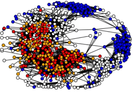
In order to obtain a ground truth community we scrape the network of @patmikekelly4 via tweepy. We scrape the list of followers for each user that follows @patmikekelly4. We then create an edge list of all of the users who follow each other while taking @patmikekelly4 out of the edge list because having one central user in the network would not occur in a terrorist recruitment network. Next, we scrape the last 300 tweets that each user published. Finally, we hand label each user into a list of ground truth communities. 8 communities are formed and all have at least 3 users. The users are members of one or more of the following communities: Bard College, the state of Massachusetts, passion for music, passion for politics, plays a sport (Athletics), plays basketball, a family member of @patmikekelly4, or computer science student/professional. For example, someone who plays music at Bard would be considered part of both the Bard and the Music ground truth communities. The data set includes 143 users. Figure 3.1 gives a visual of all of the users in the ground truth network and who they are connected with.
For the network diagrams in the following sections: A red dot means that the user is
correctly classified in the community. A blue dot means that the algorithm incorrectly classifiedthe user into it’s respective community. Anorange dot means missed classifica-tion. Missed classification means that the user is a part of the ground truth community, but
3.1. The Ground Truth Data Set 17
Figure 3.1: The Ground Truth Network. not classified as a part of that community by the algorithm.
We choose F1 scores to rank the ability of the algorithm because F1 considers both precision and the recall of the test. [2] We look at each user as a binary number telling us if that user is in the community we are examining. Precision is the number of correct positive results divided by the number of all positive results. Recall is the number of of correct positive results divided by the number of positive results that should have been returned. The F1 scores creates a weighted average of precision and recall that returns between 0 and 1. In order to rank the success of each algorithm as a whole, we calculate the average F1 score on each community and multiply it by the number of detected communities divided by the total number of ground truth communities.
18 Chapter 3. Results
3.2
The Bard Community
Figure 3.2: Bard Clique Percolation Results with F1 Score: 0.948905109489.
3.2. The Bard Community 19
Figure 3.4: Bard Combination Results with F1 Score: 0.501766784452.
The Bard community is by far the largest community in the network. Clique percolation performs extremely well for this community because of the density of it’s connections. Unfor-tunately, because of the diversity of interests amongst Bard students, it’s NMF pairing brought it’s overall F1 score down significantly. To try to improve this, future algorithms could attempt to understand that it’s dealing with a larger community which overlaps other communities, and could assign more weight to the clique percolation than to the textual clustering.
The LDA extracted topics are:
[im, gonna, literally, dying, sorry, glad, way, like, girl, eating, tired, mad, crying, really, season, date, sad, going, facebook, f*cking]
20 Chapter 3. Results
3.3
The Massachusetts Community
Figure 3.5: Massachusetts Clique Percolation Results with F1 Score: 0.786206896552.
3.3. The Massachusetts Community 21
Figure 3.7: Massachusetts Combination Results with F1 Score: 0.524390243902.
The Massachusetts community is the second largest community in the ground truth data set. Massachusetts makes up almost all of the nodes that are not a part of the Bard community. Together these two communities make up a majority of the network and both contain most of the sub communities within themselves. Once again, the NMF clustering hurts the performance that clique percolation had initially achieved, but this is expected as the topics vary greatly amongst the Massachusetts network.
The LDA extracted topics are:
[thanks, connect, follow, looking, following, miss, got, voice, lmk, time, hope, need, told, fan, congrats, best, dont, libertarians, nice, florida]
22 Chapter 3. Results
3.4
The Athletics Community
Athletics Clique Percolation Results
No athletics community detected.
3.4. The Athletics Community 23
Figure 3.9: Athletics Combination Results with F1 Score: 0.225563909774.
After Bard and Massachusetts, clique percolation isn’t expected to perform well because these communities have a lesser likelihood of being connected, and a greater likelihood of talking about similar subjects. Many of the sub-communities aren’t directly connected. As many of the athletics community members are both a part of Bard and Massachusetts, clique percolation couldn’t possibly detect their membership as they are not directly connected. NMF performs well in finding athletes referring to similar topics.
The LDA extracted topics are:
[love, people, thank, ty, life, today, free, advisor, probably, rarely, mom, hope, bro, youre, pic, bard, thing, obamas, ur, culture]
24 Chapter 3. Results
3.5
The Music Community
Figure 3.10: Music Clique Percolation Results with F1 Score: 0.
3.5. The Music Community 25
Figure 3.12: Music Combination Results with F1 Score: .201293491293.
Clique percolation is unable to detect the actual music community. NMF performs well on this community with an F1 score of .29.
LDA extracted topics are:
[home, hvac, ecolife, life, eco, protection, help, heating, comfort, water, air, energy, new, furnace, costs, save, comfortable, make, systems, sure]
26 Chapter 3. Results
3.6
The Family Community
Figure 3.13: Family Cliaue Percolation Results with F1 Score: 0.615384615385.
3.6. The Family Community 27
Figure 3.15: Family Combination Results with F1 Score: 0.585384615385.
Members of @patmikekelly14’s family are detected at a surprisingly high rate. This tiny community is detected very well by clique percolation, probably due to it’s nature of being a small community which are densely connected and not connected to the large communities that make up a majority of the network. NMF achieved minor success.
LDA extracted topics are:
[just, like, think, man, dude, did, going, got, really, lol, idea, boss, fight, roommate, years, mother, past, team, dont, stop]
28 Chapter 3. Results
3.7
The Politics Community
Figure 3.16: Politics Clique Percolation Results with F1 Score: 0.
Figure 3.17: Politics NMF Results with F1 Score: 0.124031007752.
Combination Results
3.8. The Basketball Community 29
With all of the political dialogue on Twitter in the past year cluttering the text data, the true passionate political users are unable to be accurately detected by NMF.
3.8
The Basketball Community
Clique Percolation Results
No basketball community detected.
30 Chapter 3. Results
Figure 3.19: Basketball Combination Results with F1 Score: 0.310344827586.
The basketball community is detected well by the NMF textual clustering, but is not detected by clique percolation. With an overall F1 score of .31, this sub-community is detected fairly well.
LDA extracted topics are:
[day, great, happy, best, photo, big, hours, good, february, finsup, makes, perfect, senior, valentines, going, weekend, new, presidentsday, tomorrow, youre]
3.9
The Computer Science Community
Clique Percolation Results
No computer science community detected.
NMF Results
3.10. Failure of BigClam and K-means 31
Figure 3.20: Computer Science Combination Results with F1 Score: 0.310344827586.
The computer science community results are the most intriguing, because while the algorithm does not recognize the community at first, the union of it’s closest matching results create a fairly accurate final community. This is possible due to the nature of the matching process in this algorithm. When deciding which sets to union, these two sets could have been the mismatched in clique percolation or in NMF, but when combined they match closest to the computer science community.
LDA extracted topics are:
[data, machinelearning, science, big, machine, learning, python, mining, miningtechniques, bruce, analytics, bigdata, hadoop, datascience, ai, know, power, datamining, scientist, better]
3.10
Failure of BigClam and K-means
To illustrate the difficulty that our community detection problem presents by our definition of community, we share the results of the BigClam (Network Structure) and K-Means (Textual Clustering). The BigClam algorithm failed to detect any communities with an F1 score of higher than .19. Visually, the easiest community to detect would be the Bard community, as it
32 Chapter 3. Results
is the biggest and most densely connected community. Since the bigclam attempts to maximize the likelihood of the matrix F using sets of neighbors and non-neighbors to understand the network, we expect the Bard community to be an easy find for the BigClam. The algorithm produces almost identical sets of users in the Snap Stanford C Library version and our python implementation. Figure 3.21 displays the results of the python implementation for the Bard community.
Figure 3.21: BigClam Bard Community Results with F1 Score: .461929432.
We hoped to build a mathematical model on top of the BigClam because not only does it offer overlapping community detection at scale, but it also returns a matrix F which gives a metric representing confidence in the grouping of each user. Fu in the resulting matrix offers a
non-negative scoring of how well the user fits into each community where each community is a different column in the matrix F.
Dimensionality reduction and k-means clustering also failed to utilize the tweets to group users into something close to the ground truth communities. There are two possibilities for why k-means failed to recognize clusters of users given the tweets. The data could have been non-spherical. The nature of K-means utilizing euclidean distance fails to find non-spherical clusters, whereas other algorithms can detect patterns in the data and can find non-spherical clusters.
3.11. Average F1 Scores by Algorithm 33
K-means also struggles with clusters of differing sizes. As K-means attempts to minimize the within-cluster sum of squares, larger clusters are split because they are given more weight and it ends up splitting the cluster. K-means and PCA produce an extremely low average F1 score on our ground truth data set.
3.11
Average F1 Scores by Algorithm
An average F1 score is calculated by multiplying the average F1 score of the detected commu-nities and multiplying that by the number of commucommu-nities detected by 8, the total number of communities.
Algorithm Clique Percolation NMF Text Clustering Combined Algorithms
Equation 0.39915684431167 * 6/8 0.24766934442273 * 6/8 0.37043279809681 * 7/8
Score 0.2993676332337525 0.1857520083170475 0.32412869833470875
3.12
Results on ISIS Data set
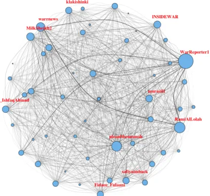
For the ISIS recruiting data set there ended up being 8 Communities formed by 4 clique percolation communities and 7 NMF communities. After set comparison, we end up with 8 communities detected. Because we have no knowledge of the true communities, presenting the list of users grouped by the algorithm is unnecessary. Instead we display the terms extracted from these communities by LDA:
Topics in Community 1: [http, english, new, sheikh, al, video, statement, wilayat, mte2, jn, ha, coming, soon, regarding, time, media, el, town, wilayataljazirah, people]
Topics in Community 2: [isis, killed, iraq, army, ramadi, soldiers, iraqi, attack, today, west, deirezzor, near, claims, breakingnews, forces, fighters, militants, islamicstate, breaking, huge]
Topics in Community 3: [allah, protect, ya, azzawajal, muslims, brothers, swt, akbar, make, help, people, said, family, accept, freemuslimprisoners, messenger, love, dua, reward, abu]
34 Chapter 3. Results
russian, deirezzor, opposition, people, kids, idlib, madaya, homs, children, assads, kerry]
Topics in Community 5: [know, did, dont, al, just, fact, shia, caliphate, ottomon, islam, muslims, want, used, didnt, world, created, america, ummah, sheikh, religion]
Topics in Community 6: [follow, brother, sisters, account, khair, support, dear, spread, true, path, jazakallah, baqiyah, shout, family, nation, great, jazakallahu, retweet, surprise, dm]
Topics in Community 7: [akhi, jazakallahu, ya, shout, im, nasheed, dm, sheikh, happened, know, link, inschallah, check, source, khair, better, plz, akh, punishment, surprise]
Topics in Community 8: [state, islamic, fighters, israel, military, says, territory, group, at-tacks, time, turkish, soldiers, terrorist, enter, explosive, sinai, wilayatsalahuddin, iraq, general, spy]
With closeness centrality[10], we discover the central figures for each ISIS recruiting community. The central figures for each ISIS community: Community 1: @WarReporter1
Community 2: @KhalidMaghrebi Community 3: @UncleSamCoco Community 4: @GunsandCoffee70 Community 5: @RamiAlLolah Community 6: @KhalidMaghrebi Community 7: @Nidalgazaui Community 8: @ismailmahsud
Chapter 4
Conclusion
4.1
Summary of Thesis Achievements
Our combination of algorithms was able to detect sub-communities in a network with a score of 0.32412869833470875 which is strong considering the difficulty of the problem. The average score is slightly stronger than both the clique percolation and NMF textual clustering, which shows that our algorithm is able to effectively combine both forms of the given data to aid in the community detection problem.
We also demonstrate the difficulty of our problem by displaying the failure of BigClam and K-Means textual on the ground truth data set. Both K-Means and BigClam have proven to be successful when applied to simpler data on large networks.
4.2
Applications
This algorithm can be applied to detect communities in a network in which the users have textual attributes such as tweets. When applied to the ISIS twitter network, we are able to group them into sub-communities, summarize what each community is discussing, and learn about who the users are. Marketing agencies may have an interest in this algorithm to improve
36 Chapter 4. Conclusion
their ability to target customers in particular communities given limited data.
4.3
Future Work
With a larger ground truth data set in a larger network, a more thorough evaluation can occur on how to best deal with the problem of community detection in networks with nodes with textual attributes. Given that there are an immense amount of algorithms that could deal with a problem of this nature, more combinations of network clustering and text clustering algorithms could be applied using our set matching process.
Further, the model could be enhanced by extending the algorithms to handle the dynamics in the networks and to detect the evolutions of communities along with the time. Understanding the shaping of a network can allow an algorithm to better understand the network’s communi-ties. Several studies have been devoted to such extensions without much success, but with the added textual data, better results may appear.
Finally and most importantly, building a model that allows the network analysis and text analysis to occur simultaneously would most likely produce stronger results than what we see with our set matching. We could not build a dynamic model due to the failure of the Bigclam on our data set. Our thesis illustrates that putting time into building a single model that would combine network science and text analysis to detect communities in networks would likely be worthwhile and produce strong results.
Bibliography
[1] Ng A., Blei D., and Jordan M. “Latent Dirichlet Allocation”. In: Journal of Machine Learning Research (2003).
[2] Orman G. et al. “On Accuracy of Community Structure Discovery Algorithms”. In: Jour-nal of Convergence Information Technology (2011).
[3] Nyi I.D., Palla G., and Vicseki T. “Clique Percolation in Random Networks”. In:Physical Review Letters (2005).
[4] Ramos J. “Using TF-IDF to Determine Word Relevance in Document Queries”. In: Pro-ceedings of the first instructional conference on machine learning. (2003).
[5] Shlens J. “A Tutorial on Principal Component Analysis”. In: Google Research (2014). [6] Yang J. and Leskovec J. “Overlapping Community Detection at Scale: A Nonnegative
Matrix Factorization Approach”. In:Web Search and Data Mining (2013), pp. 1–9. [7] Yang J., Mcauley J., and Leskovec J. “Community Detection in Networks with Node
Attributes”. In:Stanford University (2015), pp. 4–5.
[8] Girvan M. and Newman M.E.J. “Community Structure in Social and Biological Net-works”. In: Physics Abstract Service (2002), pp. 1–5.
[9] Kay M.Generating a network graph of Twitter followers using python and networkx. 2014.
url: http://mark- kay.net/2014/08/15/network- graph- of- twitter- followers/ (visited on 12/30/2016).
[10] Newman M.Networks: An Introduction. Oxford University Press, Inc., 2010.
38 BIBLIOGRAPHY
[11] Rousseeuw P. “Silhouettes: a graphical aid to the interpretation and validation of cluster analysis”. In:Journal of Computational and Applied Mathematics (1986).
[12] Li T. and Ding C. “Non-negative Matrix Factorizations for Clustering: A Survey”. In:
Appendix A
The BigClam Python Implementation
i m p o r t numpy a s np i m p o r t n e t w o r k x a s nx i m p o r t m a t p l o t l i b . p y p l o t a s p l t i m p o r t community i m p o r t math i m p o r t i t e r t o o l s a s IT i m p o r t s c i p y #A c u t , v e r t e x c u t , o r s e p a r a t i n g s e t o f a c o n n e c t e d g r a p h G #i s a s e t o f v e r t i c e s whose r e m o v a l r e n d e r s G d i s c o n n e c t e d . d e f c u t s i z e (G, S , T=None , w e i g h t=None ) : e d g e s = nx . e d g e b o u n d a r y (G, S , T) r e t u r n sum ( w e i g h t f o r u , w e i g h t i n e d g e s ) #t h e d e g r e e o f e a c h node i n t h e g r a p h d e f volume (G, S , w e i g h t=None ) : d e g r e e = G. d e g r e e d i c t V o l = d e g r e e ( S , w e i g h t=w e i g h t ) summ = [ ] f o r key , v a l u e i n d i c t V o l . i t e m s ( ) : summ . append ( v a l u e ) r e t u r n sum (summ)
#number o f c u t e d g e s / min ( volume o f t h e s e t , volume o f o t h e r s e t ) d e f c o n d u c t a n c e (G, S , T=None , w e i g h t=None ) : i f T i s None : T = s e t (G) − s e t ( S ) n u m c u t e d g e s = c u t s i z e (G, S , T , w e i g h t=w e i g h t ) v o l u m e S = volume (G, S , w e i g h t=w e i g h t ) volume T = volume (G, T , w e i g h t=w e i g h t ) r e t u r n n u m c u t e d g e s / min ( v o l u m e S , volume T ) #k = INIT method = b i g c l a m i n i t . py k = 7 F = np . z e r o s ( ( l e n ( l s ) , k ) ) c= {} # i n i t i a l i z e t h e m a t r i x F d e f g r a p h C o n d u c t a n c e (G ) : f o r w i n s e t (G ) : newSet = s e t (G. n e i g h b o r s (w ) ) c [ w ] = ( c o n d u c t a n c e (G, newSet ) ) nx . s e t n o d e a t t r i b u t e s (G, ’ c o n d u c t a n c e ’ , c ) l o c a l G r a p h = G 39
40 Appendix A. The BigClam Python Implementation
f o r i i n r a n g e ( 1 , k ) :
com = nx . g e t n o d e a t t r i b u t e s (G, ’ c o n d u c t a n c e ’ ) comNode = min ( com , k e y=com . g e t )
community = G. n e i g h b o r s ( comNode ) + [ comNode ] G = s e t (G)−s e t ( community ) f o r x i n r a n g e ( l e n ( l o c a l G r a p h . n o d e s ( ) ) ) : i f x i n community : F [ x−1 ] [ k−2] = 1 i f x i n G: F [ x−1 ] [ k−1] = 1 r e t u r n ( F ) #i t e r a t i n g t h r o u g h t h e e d g e s o f Graph . #A s s i g n 1 node a s u and 1 a s v . F = g r a p h C o n d u c t a n c e ( Graph ) n o d e s = Graph . n o d e s ( ) #o r t h o g o n a l d o t p r o d u c t t r y and f i n a l l y d e f c a t c h I n f ( e x p o n e n t i a l ) : e = np . l o g (1−e x p o n e n t i a l ) i f e == f l o a t ( ’−i n f ’ ) : r e t u r n −10 e l s e : r e t u r n e #l o o p s t h r o u g h t h e e d g e s o f t h e g r a p h #t h e L i k e l i h o o d o f t h e e n t i r e m a t r x i F #t h e s c a l a r g i v e n h e r e i s o u r o v e r a l l #l i k e l i h o o d f o r e a c h l o o p i t e r a t i o n t h r o u g h t h e e n t i r e m a t r i x . #t h i s l o o p w i l l r u n u n t i l t h e l i k e l i h o o d s t a y s t h e same l F = [ ] d e f l i k e l i h o o d O f F ( Graph ) : f o r node i n Graph . e d g e s ( ) : # u = a node f r o m t h e e d g e u = node [ 0 ] # v = a n o t h e r node f r o m t h e e d g e v = node [ 1 ] #g r a b s t h e Fu Row f r o m c o n n e c t i o n s t r e n g t h m a t r i x F Fu = F [ u−1 , : ] #same t h i n g f o r Fv Fv = F [ v−1 , : ] FvT = np . t r a n s p o s e ( Fv ) # d o t p r o d u c t o f Fu , FvT mFuFvT = np . d o t ( Fu , FvT ) #e x p o n e n t i a l o f Fu . Fv
e x p V a l = math . exp (−mFuFvT) f V a l = c a t c h I n f ( e x p V a l ) #f V a l = ( np . l o g (1−e x p V a l ) ) l F . append ( f V a l ) sLF = sum ( l F ) #now t h e c o m p l i m e n t s e t nLF = [ ] nonEdges = l i s t ( nx . n o n e d g e s ( Graph ) ) f o r node i n nonEdges : nU = node [ 0 ] nV = node [ 1 ] nFu = F [ nU−1 , : ] nFv = F [ nV−1 , : ] nFvT = np . t r a n s p o s e ( nFv ) nmFuFvT = np . d o t ( nFu , nFvT ) nLF . append (nmFuFvT) snLF = sum ( nLF ) l i k e = sLF− snLF
41 r e t u r n l i k e #l o o p s t h r o u g h e a c h node , #and t h e n t h e n e i g h b o r s f o r e a c h node d e f l i k e l i h o o d O f F u ( Graph , node ) : n e i g h L i k e = [ ] n o n N e i g h L i k e = [ ] f o r n e i g h b o r i n Graph . n e i g h b o r s ( node ) : u = node v = n e i g h b o r Fu = F [ u−1 , : ] Fv = F [ v−1 , : ] FvT = np . t r a n s p o s e ( Fv ) mFuFvT = np . d o t ( Fu , FvT )
e x p V a l = math . exp (−mFuFvT) f V a l = c a t c h I n f ( e x p V a l ) n e i g h L i k e . append ( f V a l )
#l o o p t h r o u g h non−n e i g h b o r s o f node u lSum = sum ( n e i g h L i k e )
f o r non i n nx . n o n n e i g h b o r s ( Graph , node ) : u = node v = non Fu = F [ u−1 , : ] Fv = F [ v−1 , : ] FvT = np . t r a n s p o s e ( Fv ) mFuFvT = np . d o t ( Fu , FvT ) n o n N e i g h L i k e . append (mFuFvT) nLSum = sum ( n o n N e i g h L i k e ) fLSum = lSum− nLSum r e t u r n fLSum
d e f divExp ( divNum ) :
f u n c = 1− math . exp ( divNum ) r e t u r n f u n c #c o m p u t i n g t h e g r a d i e n t d e f c o m p u t e G r a d i e n t ( Graph , node ) : n e i g h L i k e = [ ] n o n N e i g h L i k e = [ ] f o r n e i g h b o r i n Graph . n e i g h b o r s ( node ) : u = node v = n e i g h b o r Fu = F [ u−1 , : ] Fv = F [ v−1 , : ] FvT = np . t r a n s p o s e ( Fv ) mFuFvT = np . d o t ( Fu , FvT )
e x p V a l = math . exp (−mFuFvT) d i v V a l = math . exp (−mFuFvT) i f d i v V a l == 1 : o n e M i n u s D i v V a l = 1 e l s e : o n e M i n u s D i v V a l = 1 − d i v V a l f E x p V a l = e x p V a l / o n e M i n u s D i v V a l f v P r o d = np . m u l t i p l y ( Fv , f E x p V a l ) n e i g h L i k e . append ( f v P r o d ) sumFvProd = sum ( n e i g h L i k e )
f o r non i n nx . n o n n e i g h b o r s ( Graph , node ) : v = non Fv = F [ v−1 , : ] n o n N e i g h L i k e . append ( Fv ) sumOfFv = sum ( n o n N e i g h L i k e ) g r a d i e n t = sumFvProd− sumOfFv r e t u r n g r a d i e n t
42 Appendix A. The BigClam Python Implementation a l p h a = . 0 0 1 m a x I t e r = 1 0 0 0 t h r e s = . 0 0 0 1 c u r L = 0 . 0 i = 0 d e f getCommunity ( rowNum ) : rowData = V [ rowNum ] com = rowData . argmax ( )
r e t u r n com d e f b a c k T r a c k i n g L i n e S e a r c h ( theGraph , a l p h a ) : s t e p S i z e = 1 f o r i i n r a n g e ( m a x I t e r ) : f o r node i n Graph . n o d e s ( ) : d e l t a V = c o m p u t e G r a d i e n t ( Graph , node ) com = getCommunity ( node−1)
newVal = s t e p S i z e ∗ d e l t a V [ com ] i f newVal < minVal :
newVal = minVal i f newVal > maxVal : newVal = maxVal
s V a l = np . d o t ( c o m p u t e G r a d i e n t ( Graph , node ) , l i k e l i h o o d O f F u ( Graph , node ) )
i f l i k e l i h o o d O f F u ( Graph , node ) < i n i t L i k e l i h o o d + a l p h a ∗ s t e p S i z e ∗ s V a l [ com ] : s t e p S i z e = s t e p S i z e ∗ B et a e l s e : b r e a k i f i == m a x I t e r−1: s t e p S i z e = 0 . 0 r e t u r n s t e p S i z e d e f bigClam ( Graph ) : w h i l e i < m a x I t e r : i = i + 1 #g e t l i k e l i h o o d b e f o r e u p d a t e p r e v L = l i k e l i h o o d O f F ( Graph ) f o r node i n Graph . n o d e s ( ) : #c = community #u p d a t e m a t r i x w i t h g r a d i e n t f o r c i n r a n g e ( 0 , k ) : g r a d = c o m p u t e G r a d i e n t ( Graph , node ) v a l = a l p h a ∗ g r a d [ c ] u p d a t e = F [ node−1 , c ] + v a l #k e e p m a t r i x b e t w e e n 0 and 1 i f u p d a t e<= 0 : F [ node−1 , c ] = 0 e l i f u p d a t e>= 1 : F [ node−1 , c ] = 1 e l s e : F [ node−1 , c ] = u p d a t e #c u r r e n t l i k e l i h o o d c u r L = l i k e l i h o o d O f F ( Graph ) i f c u r L− p r e v L<= t h r e s∗a b s ( p r e v L ) : b r e a k e l s e : p r e v L = c u r L a l p h a = b a c k T r a c k i n g L i n e S e a r c h ( Graph , a l p h a ) p r i n t ( ’ i t e r a t i o n : ’ , i , c u r L ) p r i n t ( F )
Appendix B
Generating a Ground Truth Data Set
From Twitter
B.1
getFollowers.py
#r u n t h i s f i l e i n t e r m i n a l and name i t g e t f o l l o w e r s . py
#Get t h e k e y / t o k e n f r o m OAuth and e n t e r y o u r own u s e r n a m e i n t o t h e #s c r e e n name f i e l d #W i l l p r i n t a l i s t o f t h e u s e r IDs o f y o u r f o l l o w e r s on t w i t t e r i m p o r t t i m e i m p o r t t w e e p y c k e y = ’ ’ c s e c r e t = ’ ’ a t o k e n = ’ ’ a t o k e n s e c r e t = ’ ’ a u t h = t w e e p y . OAuthHandler ( c k e y , c s e c r e t ) a u t h . s e t a c c e s s t o k e n ( a t o k e n , a t o k e n s e c r e t ) a p i = t w e e p y . API ( a u t h ) i d s = [ ] f o r p a g e i n t w e e p y . C u r s o r ( a p i . f o l l o w e r s i d s , s c r e e n n a m e =” p a t m i k e k e l l y 4 ” ) . p a g e s ( ) : i d s . e x t e n d ( p a g e ) t i m e . s l e e p ( 2 0 ) p r i n t ( i d s )
B.2
getTheTweets.py
#name t h i s f i l e : g e t T h e T w e e t s . py #e n t e r t h e l i s t o f u s e r i d s t h a t you c r e a t e d w i t h #g e n e r a t e n e t w o r k . py i n t o t h e l i s t named ” i d s ” #t h i s c o d e w i l l c r e a t e a CSV c o n t a i n i n g a l l o f t h e #u s e r s t w e e t s a s s o c i a t e d w i t h t h e i r u s e r I D 4344 Appendix B. Generating a Ground Truth Data Set From Twitter i m p o r t t w e e p y i m p o r t c s v i m p o r t p a n d a s a s pd #Put y o u r l i s t o f u s e r i d s i n h e r e : i d s = [ ] #T w i t t e r API c r e d e n t i a l s c o n s u m e r k e y = ”” c o n s u m e r s e c r e t = ”” a c c e s s k e y = ”” a c c e s s s e c r e t = ”” #a u t h o r i z e t w i t t e r , i n i t i a l i z e t w e e p y a u t h = t w e e p y . OAuthHandler ( c o n s u m e r k e y , c o n s u m e r s e c r e t ) a u t h . s e t a c c e s s t o k e n ( a c c e s s k e y , a c c e s s s e c r e t ) a p i = t w e e p y . API ( a u t h ) o u t t w e e t s = [ ] d e f g e t a l l t w e e t s ( s c r e e n n a m e ) : #T w i t t e r o n l y a l l o w s a c c e s s t o a u s e r s most r e c e n t #3240 t w e e t s w i t h t h i s method # i n i t i a l i z e a l i s t t o h o l d a l l t h e t w e e p y Tweets a l l t w e e t s = [ ] n e w t w e e t s = a p i . u s e r t i m e l i n e ( s c r e e n n a m e = s c r e e n n a m e , c o u n t =200) f o r t w e e t i n n e w t w e e t s : o u t t w e e t s . append ( ( t w e e t . i d s t r , t w e e t . t e x t . e n c o d e ( ” u t f−8 ” ) ) ) r e t u r n o u t t w e e t s a l l o f t h e m = [ ] f o r u s e r i n i d s : t r y : u = a p i . g e t u s e r ( u s e r ) t w e e t s = g e t a l l t w e e t s ( u . s c r e e n n a m e ) a l l o f t h e m . append ( t w e e t s ) e x c e p t t w e e p y . TweepError a s e : p a s s w i t h open ( ’ a l l t w e e t s . c s v ’ , ’w ’ ) a s f i l e : o u t p u t = c s v . w r i t e r ( f i l e , d e l i m i t e r = ’ , ’ ) o u t p u t . w r i t e r o w s ( [ [ ’ i d ’ , ’ t w e e t ’ ] ] ) #a f t e r r u n n i n g t h i s f i l e you w i l l h a v e a l i s t o f u s e r i d s , and a # l i s t o f t h e l a s t x number o f t w e e t s t h a t e a c h u s e r composed .
B.3
buildNetwork.py
This code is based off of the tutorial written by [9] and modified to fit our needs. #T h i s c o d e w i l l g e n e n a t e JSONs f o r e a c h u s e r c o n t a i n i n g #a l i s t o f who e a c h u s e r i s f o l l o w i n g w i t h up t o 4 0 0 u s e r s f o r e a c h . i m p o r t t w e e p y i m p o r t t i m e i m p o r t o s i m p o r t s y s i m p o r t j s o n i m p o r t a r g p a r s e FOLLOWING DIR = ’ f o l l o w i n g ’
B.3. buildNetwork.py 45
MAX FRIENDS = 4 0 0
FRIENDS OF FRIENDS LIMIT = 4 0 0 i f n o t o s . p a t h . e x i s t s (FOLLOWING DIR ) : o s . m a k e d i r (FOLLOWING DIR) e n c = lambda x : x . e n c o d e ( ’ a s c i i ’ , e r r o r s = ’ i g n o r e ’ ) CONSUMER KEY = ’ ’ CONSUMER SECRET = ’ ’ ACCESS TOKEN = ’ ’ ACCESS TOKEN SECRET = ’ ’ # == OAuth A u t h e n t i c a t i o n ==
# T h i s mode o f a u t h e n t i c a t i o n i s t h e new p r e f e r r e d way # o f a u t h e n t i c a t i n g w i t h T w i t t e r .
a u t h = t w e e p y . OAuthHandler (CONSUMER KEY, CONSUMER SECRET) a u t h . s e t a c c e s s t o k e n (ACCESS TOKEN, ACCESS TOKEN SECRET) a p i = t w e e p y . API ( a u t h )
d e f g e t f o l l o w e r i d s ( c e n t r e , max depth =1 , c u r r e n t d e p t h =0 , t a b o o l i s t = [ ] ) : # p r i n t ’ c u r r e n t d e p t h : %d , max d e p t h : %d ’ % ( c u r r e n t d e p t h , max depth ) # p r i n t ’ t a b o o l i s t : ’ , ’ , ’ . j o i n ( [ s t r ( i ) f o r i i n t a b o o l i s t ] ) i f c u r r e n t d e p t h == max depth : p r i n t ( ’ o u t o f depth ’ ) r e t u r n t a b o o l i s t i f c e n t r e i n t a b o o l i s t : # we ’ v e b e e n h e r e b e f o r e p r i n t ( ’ A l r e a d y b e e n h e r e . ’ ) r e t u r n t a b o o l i s t e l s e : t a b o o l i s t . append ( c e n t r e ) t r y : u s e r f n a m e = o s . p a t h . j o i n ( ’ t w i t t e r−u s e r s ’ , s t r ( c e n t r e ) + ’ . j s o n ’ ) i f n o t o s . p a t h . e x i s t s ( u s e r f n a m e ) : p r i n t ( ’ R e t r i e v i n g u s e r d e t a i l s f o r t w i t t e r i d %s ’ % s t r ( c e n t r e ) ) w h i l e True : t r y : u s e r = a p i . g e t u s e r ( c e n t r e ) d = {’ name ’ : u s e r . name , ’ s c r e e n n a m e ’ : u s e r . s c r e e n n a m e , ’ i d ’ : u s e r . i d , ’ f r i e n d s c o u n t ’ : u s e r . f r i e n d s c o u n t , ’ f o l l o w e r s c o u n t ’ : u s e r . f o l l o w e r s c o u n t , ’ f o l l o w e r s i d s ’ : u s e r . f o l l o w e r s i d s ( )} w i t h open ( u s e r f n a m e , ’w ’ ) a s o u t f : o u t f . w r i t e ( j s o n . dumps ( d , i n d e n t =1)) u s e r = d b r e a k e x c e p t t w e e p y . TweepError a s e r r o r : p r i n t ( t y p e ( e r r o r ) ) i f s t r ( e r r o r ) == ’ Not a u t h o r i z e d . ’ : p r i n t ( ’ Can ’ ’ t a c c e s s u s e r d a t a − n o t a u t h o r i z e d . ’ ) r e t u r n t a b o o l i s t i f s t r ( e r r o r ) == ’ U s e r h a s b e e n s u s p e n d e d . ’ : p r i n t ( ’ U s e r s u s p e n d e d . ’ ) r e t u r n t a b o o l i s t e r r o r O b j = e r r o r [ 0 ] [ 0 ] p r i n t ( e r r o r O b j ) i f e r r o r O b j [ ’ m e s s a g e ’ ] == ’ Rate l i m i t e x c e e d e d ’ : p r i n t ( ’ Rate l i m i t e d . S l e e p i n g f o r 15 m i n u t e s . ’ ) t i m e . s l e e p ( 1 5 ∗ 60 + 1 5 ) c o n t i n u e r e t u r n t a b o o l i s t e l s e :
46 Appendix B. Generating a Ground Truth Data Set From Twitter
u s e r = j s o n . l o a d s ( f i l e ( u s e r f n a m e ) . r e a d ( ) ) s c r e e n n a m e = e n c ( u s e r [ ’ s c r e e n n a m e ’ ] )
fname = o s . p a t h . j o i n (FOLLOWING DIR, s c r e e n n a m e + ’ . c s v ’ ) f r i e n d i d s = [ ] # o n l y r e t r i e v e f r i e n d s o f Pat . . . s c r e e n names i f s c r e e n n a m e ==(’ p a t m i k e k e l l y 4 ’ ) : i f n o t o s . p a t h . e x i s t s ( fname ) : p r i n t ( ’ No c a c h e d d a t a f o r s c r e e n name ”%s ” ’ % s c r e e n n a m e ) w i t h open ( fname , ’w ’ ) a s o u t f : params = ( e n c ( u s e r [ ’ name ’ ] ) , s c r e e n n a m e ) p r i n t ( ’ R e t r i e v i n g f r i e n d s f o r u s e r ”%s ” (% s ) ’ % params ) # p a g e o v e r f r i e n d s c = t w e e p y . C u r s o r ( a p i . f r i e n d s , i d=u s e r [ ’ i d ’ ] ) . i t e m s ( ) f r i e n d c o u n t = 0 w h i l e True : t r y : f r i e n d = c . n e x t ( ) f r i e n d i d s . append ( f r i e n d . i d ) params = ( f r i e n d . i d , e n c ( f r i e n d . s c r e e n n a m e ) , e n c ( f r i e n d . name ) ) o u t f . w r i t e ( ’% s\t%s\t%s\n ’ % params ) f r i e n d c o u n t += 1 i f f r i e n d c o u n t >= MAX FRIENDS : p r i n t ( ’ Reached max no . o f f r i e n d s f o r ”%s ” . ’ % f r i e n d . s c r e e n n a m e ) b r e a k e x c e p t t w e e p y . TweepError : # h i t r a t e l i m i t , s l e e p f o r 15 m i n u t e s p r i n t ( ’ Rate l i m i t e d . S l e e p i n g f o r 15 m i n u t e s . ’ ) t i m e . s l e e p ( 1 5 ∗ 60 + 1 5 ) c o n t i n u e e x c e p t S t o p I t e r a t i o n : b r e a k e l s e : f r i e n d i d s = [ i n t ( l i n e . s t r i p ( ) . s p l i t ( ’\t ’ ) [ 0 ] ) f o r l i n e i n f i l e ( fname ) ] p r i n t ( ’ Found %d f r i e n d s f o r %s ’ % ( l e n ( f r i e n d i d s ) , s c r e e n n a m e ) ) # g e t f r i e n d s o f f r i e n d s cd = c u r r e n t d e p t h i f cd+1< max depth :
f o r f i d i n f r i e n d i d s [ : FRIENDS OF FRIENDS LIMIT ] :
t a b o o l i s t = g e t f o l l o w e r i d s ( f i d , max depth=max depth , c u r r e n t d e p t h=cd +1 , t a b o o l i s t = t a b o o l i s t )
i f cd+1< max depth and l e n ( f r i e n d i d s ) > FRIENDS OF FRIENDS LIMIT : p r i n t ( ’ Not a l l f r i e n d s r e t r i e v e d f o r %s . ’ % s c r e e n n a m e ) e x c e p t E x c e p t i o n a s e r r o r : p r i n t ( ’ E r r o r r e t r i e v i n g f o l l o w e r s f o r u s e r i d : ’ , c e n t r e ) p r i n t ( e r r o r ) i f o s . p a t h . e x i s t s ( fname ) : o s . remove ( fname ) p r i n t ( ’ Removed f i l e ”%s ” . ’ % fname ) s y s . e x i t ( 1 ) r e t u r n t a b o o l i s t i f n a m e == ’ m a i n ’ : ap = a r g p a r s e . A r g u m e n t P a r s e r ( )
ap . a d d a r g u m e n t (”−s ” , ”−−s c r e e n−name ” , r e q u i r e d=True , h e l p =” S c r e e n name o f t w i t t e r u s e r ” ) ap . a d d a r g u m e n t (”−d ” , ”−−d e p t h ” , r e q u i r e d=True , t y p e=i n t , h e l p =”How f a r t o f o l l o w u s e r n e t w o r k ” ) a r g s = v a r s ( ap . p a r s e a r g s ( ) )
t w i t t e r s c r e e n n a m e = a r g s [ ’ s c r e e n n a m e ’ ] d e p t h = i n t ( a r g s [ ’ depth ’ ] )
i f d e p t h < 1 o r d e p t h > 3 :
B.4. twitterNetwork.py 47 s y s . e x i t ( ’ I n v a l i d d e p t h argument . ’ ) p r i n t ( ’ Max Depth : %d ’ % d e p t h ) m a t c h e s = a p i . l o o k u p u s e r s ( s c r e e n n a m e s =[ t w i t t e r s c r e e n n a m e ] ) i f l e n ( m a t c h e s ) == 1 : p r i n t ( g e t f o l l o w e r i d s ( m a t c h e s [ 0 ] . i d , max depth=d e p t h ) ) e l s e : p r i n t ( ’ S o r r y , c o u l d n o t f i n d t w i t t e r u s e r w i t h s c r e e n name : %s ’ % t w i t t e r s c r e e n n a m e )
B.4
twitterNetwork.py
This is the last step in the process. This code takes the central user out of the network, and creates an edge list in a CSV of who is following who from the user list.
i m p o r t g l o b i m p o r t o s i m p o r t j s o n i m p o r t s y s f r o m c o l l e c t i o n s i m p o r t d e f a u l t d i c t u s e r s = d e f a u l t d i c t ( lambda : { ’ f o l l o w e r s ’ : 0 }) f o r f i n g l o b . g l o b ( ’ t w i t t e r−u s e r s /∗. j s o n ’ ) : d a t a = j s o n . l o a d ( f i l e ( f ) ) s c r e e n n a m e = d a t a [ ’ s c r e e n n a m e ’ ] u s e r s [ s c r e e n n a m e ] = { ’ f o l l o w e r s ’ : d a t a [ ’ f o l l o w e r s c o u n t ’ ] } SEED = ’ p a t m i k e k e l l y 4 ’ d e f p r o c e s s f o l l o w e r l i s t ( s c r e e n n a m e , e d g e s = [ ] , d e p t h =0 , max depth = 2 ) : f = o s . p a t h . j o i n ( ’ f o l l o w i n g ’ , s c r e e n n a m e + ’ . c s v ’ ) i f n o t o s . p a t h . e x i s t s ( f ) : r e t u r n e d g e s f o l l o w e r s = [ l i n e . s t r i p ( ) . s p l i t ( ’\t ’ ) f o r l i n e i n f i l e ( f ) ] f o r f o l l o w e r d a t a i n f o l l o w e r s : i f l e n ( f o l l o w e r d a t a ) < 2 : c o n t i n u e s c r e e n n a m e 2 = f o l l o w e r d a t a [ 1 ] # u s e t h e number o f f o l l o w e r s f o r s c r e e n n a m e a s t h e w e i g h t w e i g h t = u s e r s [ s c r e e n n a m e ] [ ’ f o l l o w e r s ’ ] e d g e s . append ( [ s c r e e n n a m e , s c r e e n n a m e 2 , w e i g h t ] ) i f d e p t h+1 < max depth : p r o c e s s f o l l o w e r l i s t ( s c r e e n n a m e 2 , e d g e s , d e p t h +1 , max depth ) r e t u r n e d g e s
e d g e s = p r o c e s s f o l l o w e r l i s t (SEED , max depth =3) w i t h open ( ’ t w i t t e r n e t w o r k . c s v ’ , ’w ’ ) a s o u t f : e d g e e x i s t s = {} f o r e d g e i n e d g e s : k e y = ’ , ’ . j o i n ( [ s t r ( x ) f o r x i n e d g e ] ) i f n o t ( k e y i n e d g e e x i s t s ) : o u t f . w r i t e ( ’% s\t%s\t%d\n ’ % ( e d g e [ 0 ] ,
![Figure 1.2: Probabilistic Model of LDA [1].](https://thumb-us.123doks.com/thumbv2/123dok_us/853838.2608764/24.892.263.633.879.1070/figure-probabilistic-model-of-lda.webp)