A combined machine learning algorithms and DEA method for measuring and predicting the efficiency of Chinese manufacturing listed companies

1

Zhu, C., N. Zhu, and, A. Emrouznejad (2020) A combined machine learning algorithms and DEA

method for measuring and predicting the efficiency of Chinese manufacturing listed companies,

Journal of Management Science and Engineering

,

https://doi.org/10.1016/j.jmse.2020.10.001

.

A combined machine learning algorithms and DEA method for measuring and

predicting the efficiency of Chinese manufacturing listed companies

Nan Zhu

The Western Business School, Southwestern University of Finance and Economics, Chengdu, China [email protected]

Chuanjin Zhu

The School of Statistics, Southwestern University of Finance and Economics, Chengdu, China [email protected]

Ali Emrouznejad

Operations & Information Management, Aston Business School, Aston University, Birmingham, UK [email protected]

Abstract

Data Envelopment Analysis (DEA) is a linear programming methodology for measuring the efficiency of Decision Making Units (DMUs) to improve organizational performance in the private and public sectors. However, if a new DMU needs to be known its efficiency score, the DEA analysis would have to be re-conducted, especially nowadays, datasets from many fields have been growing rapidly in the real world, which will need a huge amount of computation. Following the previous studies, this paper aims to establish a linkage between the DEA method and machine learning (ML) algorithms, and proposes an alternative way that combines DEA with ML (ML-DEA) algorithms to measure and predict the DEA efficiency of DMUs. Four ML-DEA algorithms are discussed, namely DEA-CCR model combined with propagation neural network (BPNN-DEA), with genetic algorithm (GA) integrated with and back-propagation neural network (GANN-DEA), with support vector machines (SVM-DEA), and with improved support vector machines (ISVM-DEA), respectively. To illustrate the applicability of above models the performance of Chinese manufacturing listed companies in 2016 is measured, predicted and compared with the DEA efficiency scores obtained by the DEA-CCR model. The empirical results show that the average accuracy of the predicted efficiency of DMUs is about 94%, and the comprehensive performance order of four ML-DEA algorithms ranked from good to poor is GANN-DEA, BPNN-DEA, ISVM-DEA, and SVM-DEA.

2 1 Introduction

It is universally acknowledged that based on Farrell’s (1957) original work, data envelopment analysis (DEA) is a frontier analysis approach to efficiency measurement of Decision-Making Units (DMUs) with multi-inputs and multi-outputs by using a linear programming methodology, by Charnes et al. (1978). Since then new methods and applications with more variables and more complicated models are being introduced. DEA methods have been widely used in many fields for assessing efficiency of DMUs to improve organizational performance in many sectors, such as in government agencies, airlines, hospitals, financial institutions and manufacturing companies. See Emrouznejad et al. (2018) for a full bibliography of DEA.

During evaluating organizational performance, however, if a new DMU needs to be known its efficiency score, the DEA analysis would have to be re-conducted. Especially, nowadays DMU datasets are growing quickly in the real world with the rapid development of big data. For example, the number of small and micro-sized companies in mainland China has exceeded 73 million, and the number is still increasing, (Zhang, 2017). Hence, when we have already calculated DEA efficiency for a large number of DMUs, and if a new DMU needs to be known its efficiency score, the DEA model would have to be re-run, which would need huge computer resources in terms of memory and CPU time. Therefore, we attempt to propose a way to predict the efficiency score using machine learning (ML) algorithms.

ML algorithms build a mathematical model of sample data, known as “training data”, in order to make predictions or decisions without being explicitly programmed to perform the task (Bishop, 2006). It is used in the applications of evaluating organizational performance with DEA. For example, to address the problem for the very large scale datasets emerging in practice, Emrouznejad et al. (2009) proposed a neural network back-propagation DEA algorithm (NNDEA), the empirical result showed that the NNDEA prediction for efficiency score appeared to be a good estimation for the majority of DMUs, and the analysis of error showed that the larger the datasets the smaller error. Fethi et al. (2010) presented a comprehensive review of 179 studies which employed operations research (OR) and artificial intelligence (AI) techniques in the assessment of bank performance, and they found only a few studies that proposed the combination of the prediction of individual models into integrated meta-classifiers, and believed that this was an area of research that was worthy of further attention. Barros et al. (2014) and Kwon et al. (2015) proposed a DEA-BPNN method to measure and predict the efficiency score of insurance companies in Mozambique and large US banks, respectively. Misiunas et al. (2016) proposed a hybrid DEANN methodology to improve prediction with an application to predict the functional status of patients in organ transplant operations, the results demonstrated that high accuracy rates with a reduction in training datasets size validated the DEANN. Supplier assessment and selection of the high-quality

3

suppliers play a vital role in successful supply chain management, hence Fallahpour et al. (2016) employed an integrated genetic programming model to address the drawbacks of existing DEA-AI approaches in supplier selection, the results showed that the proposed approach can address the issues of DEA models in distinguishing technical efficiency and time-consuming of efficiency calculation. Gupta et al. (2016) applied a DEA approach to measure the relative energy efficiency of residential buildings, and divided the DMUs into two classes, namely efficient and inefficient. Then, they used three machine learning classification algorithms to perform classification on unseen DMUs, and made a comparative analysis of the results obtained by different classification algorithms. Yang et al. (2017) studied the problem of rule reduction in the extended belief-rule-based system (EBRBS) and applied DEA approach to assess the efficiency of each rule in an extended belief-rule-based (EBRB), the results showed that the DEA-based rule reduction approach can downsize the EBRB and promote the accuracy of EBRBS. De Clercq et al. (2019) explored the determinants of efficiency in industrial scale co-digestion facilities in the US and Germany using a combined DEA and stochastic gradient boosting approach, the results indicated that high suitability for separating the determinants of efficiency. Liu et al. (2019) evaluated the financing efficiency of 39 agricultural listed companies in China from 2013 to 2017 based on DEA method, Tobit regression model and the random forest regression model. Since most of the previous researches focused on variables that affect efficiency, rather than efficiency prediction, Nandy et al. (2020, In Press) attempted to apply DEA method in combination with Random forest (RF) algorithm to assess and predict the effect of environmental variables on the performance of farms, and the DEA-RF two-stage approach was used to 450 paddy producers in rural Eastern India. In order to find out the key factors that affect the academic performance of schools and explore the relationship between them, Rebai et al. (2020, In Press) conducted a combined DEA method with a graphically based regression trees and random forests with an application to Tunisian secondary schools, the results emphasized that the machine learning could capture the manner in which multiple mechanisms jointly shape associations between secondary schools performance and the related factors.

According to a preceding review of the above-mentioned studies, the previous literature shows that the hybrid ML-DEA methodology has received much attention for predicting the efficiency of DMUs in many fields. However, the current studies have some drawbacks, for instance, the ML algorithm is mainly limited to neural network or back-propagation neural network, there are even some studies that employ decision tree and random forest algorithm, which are not suitable for regression tasks, to predict continuous efficiency value. On the other hand, there is still a lack of researches on applying integrated models to predict efficiency and comparing the results with single models. To address the above problems, this paper has a purpose to establish a linkage between DEA method and ML algorithms, and proposes an alternative way that combines DEA with more ML (ML-DEA) algorithms to measure and predict the

4

efficiency of DMUs. Four ML-DEA algorithms are discussed: DEA-CCR model combined with back-propagation neural network (BPNN-DEA), with genetic algorithm (GA) integrated with back-back-propagation neural network (GANN-DEA), with support vector machines (SVM-DEA), and with improved support vector machines (ISVM-DEA), respectively. The BPNN and SVM are the classical algorithm, and the GANN is an integrated model that integrates the BPNN with the GA algorithm. The ISVM algorithm is proposed in this paper by adding a novel loop structure to search the best initial parameters of the model. To illustrate the applicability of proposed approach, a the real datasets of the manufacturing companies operated in mainland China in 2016 is collected, and the performances of the companies are measured, predicted and compared with the DEA efficiency scores obtained by the DEA-CCR model, respectively.

The rest of the paper is organized as follows. The DEA method and four ML algorithms are explained in

Section 2. The research framework on combining DEA method with four ML algorithms is discussed in

Section 3. In Section 4, the performances of Chinese manufacturing listed companies in 2016 are measured, predicted and compared with the efficiency scores obtained by the DEA-CCR model, respectively. Finally, Section 5 concludes this paper and provides direction for future studies.

2 Methodologies

2.1 DEA methods with applications

DEA is a method for measuring the efficiency of DMUs using linear programming methodology to ‘‘envelop” observed input/output vectors as tightly as possible. The DEA-CCR model (Charnes, et al., 1978) is a frontier analysis model concerning the ratio of multi-outputs to multi-inputs of using scarce resources to produce valuable items of a DMU subjected to the condition that the similar ratios for all other DMUs be less than or equal to one. The model does not require a priori weights on inputs and outputs.

Suppose there is a set of N DMUs. Each DMUt (t =1, ...,N) produces J different outputs yt_{j (j =1, ..., J)} utilizing I different inputs xti (i =1, ..., I); (xt, yt) is a positive known input/output vector for the DMUt. There is the fractional programming model (Charnes, et al., 1978; Cooper et al., 2004):





= = = _I i t i i J j t j j t x v y u FE 1 1 max

5

,

,

,

1

;

,

,

1

;

0

,

;

,

,

1

,

1

.

.

1 1

J

j

I

i

u

v

N

n

x

v

y

u

t

s

j i I i n i i J j n j j







=

=



=







= = (2.1)

where (v, u) is the variable input/output weight vector. The DMUt (t =1,…, N) is measured for the optimal objective value FEt with the optimal solution (v*, u* ) in (2.1). It can be proved that the model (2.1) is equivalent to the linear programming model, i.e., the input-oriented DEA-CCR model (2.2) which assumes the existence of constant returns-to-scale (CRS). The maximum, TEt (=FEt) of the objective function given by the CCR model (2.2) is called the technical efficiency (TE) of DMUt. We have TE≤ 1.

t j J j j t u y TE =



₌ 1 max

.

,

,

1

;

,

,

1

;

0

,

,

1

;

,

,

1

,

0

.

.

1 1 1

J

j

I

i

u

v

x

v

N

n

x

v

y

u

t

s

j i t i I i i n i I i i n j J j j







=

=



=

=



−







= = = (2.2)

TE can be decomposed as the product of pure technical efficiency (PTE) and scale efficiency (SE): PE = PTE × SE. See Banker et al. (1984) who extended the CCR model (2.2) to the BCC model for obtaining PTE score by assuming the existence of variable returns-to-scale (VRS). TE score expresses the global operational efficiency of a DMU, since it takes no count of scale effect, but PTE score expresses the local PTE of the DMU under VRS conditions. SE, which is obtained by PE / PTE, expresses the efficiency of operation in the productive scale size of the DMU. Generally, if the efficiency score is equal to value one then the DMU is called efficient relatively, however, if the value is less than one then the DMU is called inefficient relatively.

After the work of Charnes et al. (1978), many new applications with more variables and more complicated models are being introduced for measuring the efficiency and productivity change of DMUs so as to improve organizational performance in private and public sectors. Examples of models and applications of DEA can be seen in Cooper et al. (2004), Mulwa et al. (2008), Ray et al. (2010), Song et al. (2018), Yang et al. (2020, In Press). See also Emrouznejad et al. (2018) for a full bibliography of DEA. Due to the complexity of DEA calculation, several specialist software products have been developed (e.g., Emrouznejad, 2005).

However, during evaluating organizational performance, if a new DMU is added, the DEA model would have to be re-run. To avoid recalculation of efficiency of all DMUs, some studies proposed on predicting

6

the DEA efficiency of a new DMUs by using the DEA model combining with some ML algorithms. For example, Liu et al. (2013) used DEA, three-stage DEA and artificial neural network (ANN) to measure the technical efficiency of 29 semi-conductor firms in Taiwan area, and found that different approaches (DEA vs. NN) will produce different results when they are employed in the similar methodological framework. The DEA and SVM combination is also used to improve classification, see for examples, Jiang et al. (2013).

Nowadays, datasets have been growing quickly in the real world with the rapid development of big data. Hence, when DEA for a the large datasets with many inputs and outputs would require huge computer resources in terms of memory and CPU time. Emrouznejad et al. (2009) proposed a neural network back-propagation DEA algorithm (NNDEA). The aim of the algorithm developed is to select a random set of DMUs for training a neural network and then use the generated model for estimating the efficiency scores without any need to solve linear programming problems for every single DMU. Since that algorithm requirements for computer memory and CPU time are far less than those which are needed by the DEA-CCR model it can be a useful tool in measuring efficiency in large datasets. Misiunas et al. (2016) combined DEA with ANN, and proposed a healthcare analytic methodology for the prediction of organ recipient functional status. Their work examines the thoracic datasets that consists of 16,771 records and 442 variables containing information on all lung and heart transplants performed in the US. The methodology is implemented via the problem of predicting the functional status of patients in organ transplant operations. The results yielded are very promising which validates the proposed method.

Following the previous scholars’ work, this paper proposes an alternative way that combines DEA with four ML algorithms to predict the efficiency of DMUs. In the following subsections, four ML algorithms are discussed, respectively.

2.2 ML algorithms

The development of ML has mainly gone through three main periods: Hebb (1949) took the first step of ML based on the learning mechanism of neuropsychology, after that ML has been developed briefly. Then, the development of ML has experienced about fifteen years of stagnation from the mid-1960s to the end of the 1970s, because the limited memory and processing speed of computers at that time was not sufficient to solve any practical AI problems. Since the late 1970s, people have expanded from learning a single concept to learning multiple concepts, explored different kinds of learning strategies and various learning methods. During this period, ML returned to people’s attention and slowly recovered. Now ML attracts the attention of many scholars with the rapid development of AI and data mining, and many

7

breakthroughs have appeared already. After decades of development, ML algorithms are mainly used to solve classification, regression and cluster problems.

ML is a multi-disciplinary subject involving many disciplines such as probability theory, statistics, approximation theory, convex analysis, and algorithm complexity theory. It specializes in how computers simulate or implement human learning behaviors to acquire new knowledge or skills and reorganize existing knowledge structures to continuously improve their performance. After decades of continuous development (Turing, 1950; Rosenblatt, 1958; Werbos, 1981; Schapire, 1990; Cortes et al., 1995), nowadays ML is a well-known method that “using algorithms to parse data, learn from it, and then make decisions or predictions about something unknown in the world”. ML has been widely used in many applications, such as data mining (Kavakiotis et al., 2017), computer vision (Brunetti et al., 2018), biometric recognition (Chen et al., 2016), stock market analysis (Lee et al., 2019) and robotic applications (Xu et al., 2018), and so on.

Generally, the key of ML is using algorithms to parse data, learn from it, and then make decisions or predictions about something unknown. This means that instead of explicitly writing a program to perform certain tasks, it is better to teach the computer how to develop an algorithm to accomplish the task. ML is mainly divided into supervised learning, unsupervised learning, semi-supervised learning, and intensive learning. Each method has its specific advantages and shortcomings. The supervised learning is one of the most widely used machine learning algorithms, and the main tasks of supervised learning are classification and regression. In classification, machines are trained to divide a group into specific classes. A simple example of the classification is the spam filter on an email account. The filter analyzes emails that someone has previously marked as spam and compares them to new ones. If they match a certain percentage, these new messages will be marked as spam and sent to the appropriate folder. Emails that are not similar are classified as normal and sent to the mailbox. In regression, the machine uses previous (marked) data to predict the future. Weather applications are a good example of a return. Using historical data on weather events (i.e. average temperature, humidity, and precipitation), the mobile weather application (APP) can view current weather and predict weather in the future. For more information about ML, see Stuart et al. (2010) and Mehryar et al. (2012). Since the technical efficiency of the DEA-CCR model (2.2) is continuous data, so in this paper four ML algorithms that are fitted for regression problems are discussed. They are back-propagation neural network (BPNN), GA combined with BPNN (GANN), support vector machines (SVM) and its improved SVM (ISVM). 2.2.1 Back-propagation neural network

To introduce BPNN, it needs to start with ANNs (Mcculloch et al., 1943). In ML and cognitive science, ANNs are a family of statistical learning models inspired by biological NNs (i.e. the central nervous

8

systems of animals) and are used to estimate or approximate functions that can depend on a large number of inputs and are generally unknown. Below a brief introduction will be given to the original idea of ANNs: The single neuron model can be simplified to Figure 1, this is the simplest neuron model. This model can be taken as an example to introduce the basic idea of ANN: Assuming that there are m DMUs and each DMU has n features (i.e., n inputs, that is x1, x2 ,…, xn in Figure 1), and each DMU has a target variable y (Target variable is the object that we want to research, different research problems have different target variables, and for DMUi, its target variable can be written as yi), it also can be called output variables; For DMUi, obviously the importance of each feature is different, so each feature has different weights depending on importance (i.e., wi1, wi2, …, win in Figure 1). Then, the weighted sum of inputs and yi can establish a mapping relationship by an activation function:

𝑦𝑖 = 𝑓(∑ 𝑤𝑖𝑗𝑥𝑗) 𝑛

𝑗=0 − 𝜃 (2.3)

In (2.3)，∑𝑛𝑗=0𝑤𝑖𝑗𝑥𝑗is the weighted sum of inputs, θ is the intercept term. 𝑓() is the activation function,

there are some common activation function like sigmoid function, tanh function, rectified linear unit function (namely ReLU), softmax function, etc. By collecting n DMUs with known inputs and outputs, the weights wij and θ can be estimated according to (2.3), this step is also called model training. After getting the trained model, once the new DMU is generated, whose inputs are known but the outputs are unknown, we can get the estimated output through the model, the weights wij and θ can be corrected at the same time. The principle of the multilayer neural network model is similar to this, see more in Cheng (1995). wi0 win wi2 wi1 x1 x2 xn . . . yi ∑ f () x0 = −1

Figure 1. Diagram of single neuron model

After a long period of development, at present BPNN has become the most commonly used method of teaching ANNs how to perform a given task (Rumelhart et al. 1986). It mainly has two features: (a) It is a supervised learning method, and is a generalization of the delta rule. It requires an expert who knows, or can calculate, the desired output for any input in the training datasets. (b) It requires that the activation function used by the artificial neurons is everywhere differentiable.

9

The BPNN algorithm was developed by ANN. Because the mathematical proof process of BPNN is complicated, and many books and papers have explained it, this paper just briefly introduces its basic principles: propagation and weight update (namely, the actual output is calculated in the direction from input to output, while the modification of weights and thresholds is carried out in the direction from output to input).

Phase 1:Propagation

a. Forward propagation of a training pattern’s input through the NN in order to generate the propagation’s output activations.

b. Back-propagation of the propagation’s output activations through the NN using the training pattern’s target to generate the deltas of all output and hidden neurons.

In this phase, it needs to calculate the output value of each node. It is based on the output value of all nodes of the previous layer, the weights between the current node and all nodes of the previous layer, the current node’s threshold and activation function. One of the common activation function is a sigmoid function, and it is used as an activation function in this paper.

Phase 2:Weight Update

a. Multiply its output delta and input activation to get the gradient of the weight.

b. Bring the weight in the opposite direction of the gradient by subtracting a ration of it from the weight.

This phase is the error back-propagation process, the basic idea of BPNN is to adjust the network parameters by calculating the error between the output layer and the expected value, so that the error becomes smaller. The specific mathematical process can be seen in Rumelhart et al. (1986) and Rattay (1999), and the full code for BPNN based on MATLAB (R2016b) software can be seen in

Supplementary Materials.

2.2.2 Genetic algorithm and its integration with back-propagation neural network

GA is an evolutionary algorithm whose basic principle is to imitate the evolutionary rules of “natural selection and survival of the fittest” in the biological world, which was originally proposed by Holland (1975). The GA is a global search method, that is are based on three basic operations: selection, crossover and mutation.

The purpose of the selection is to select good individuals from the current group, so that they have the opportunity to become the descendants of the next generation to multiply the offspring, and the basis for selection is the probability that the adaptable individuals contribute one or more offspring to the next

10

generation. Through crossover, a new generation of individuals can be obtained, and the new individuals combine the characteristics of the parents. Pairs of individuals in a group are randomly paired, and for each individual, some of the chromosomes between them are exchanged with a crossover probability. For each individual in the population, the genetic value at one or more loci is changed by the mutation probability to other alleles. As in the biological world, the probability of a mutation occurring is very low, and variation provides an opportunity for the creation of new individuals.

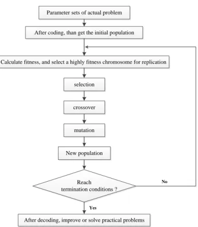
Parameter sets of actual problem

After coding, than get the initial population

Calculate fitness, and select a highly fitness chromosome for replication

selection crossover mutation New population Reach termination conditions ?

After decoding, improve or solve practical problems

Yes

No

Figure 2. The basic steps of GA

GA simulates the natural evolution of the population, and the latter population is more adaptable to the environment than the previous generation. The optimal individual in the last generation can be decode, which can be used as an approximate optimal solution, so it's an optimization algorithm. The basic steps of GA is shown in Figure 2, explanations of relevant technical terms can be found in Table 1. For more information about GA, see Vose (1999) and Schmitt (2001).

Although the BPNN has a mature theory and wide application, it still has many problems, such as the convergence rate is slow, the iterations increase, and the realtime performance is not so good. It is necessary to improve the initial BPNN to solve there problems and achieve optimal performance. Therefore, it needs to use GA to optimize the initial BPNN so as to improve the training speed of it and

11

prediction accuracy.Based on the previous work (e.g., Kitano, 1990), and the full code for GANN based on MATLAB (R2016b) software can be seen in Supplementary Materials.

2.2.3 Support vector machine and its improved algorithm

SVM is a set of related supervised learning methods that analyze data and recognize patterns, used for classification and regression analysis. The SVM algorithm was invented by Drucker et al. (1997), see also Vapnik (1993). The current standard incarnation (i.e., soft margin) was proposed by Cortes et al. (1995).

As shown in Figure 3, a the SVM constructs a hyperplane or set of hyperplanes in a high or infinite-dimensional space, which can be used for classification, regression, or other tasks. A good separation is achieved by the hyperplane that has the largest distance to the nearest training data points of any class, since in general the larger the margin the lower the generalization error of the classifier.

Maximum-margin Optimal hyperplane Cluster 1 Cluster 2 Support vector Support vector

Figure 3. A brief diagram of SVM

SVM is proposed for the problem of binary classification, it can not solve the regression problem. To address the problem, Vapnik et al. (1997) introduced the insensitive loss function on the basis of SVM classification, thus the regression SVM (SVR) is obtained. The difference between SVR and SVM classification is that the SVR samples have only one type in the end, the basic idea is not to find an optimal classification surface to separate two types of samples, but to find an optimal classification surface to minimize the error of all training samples from the optimal classification plane.

SVR is divided into linear and non-linear regression (Vapnik et al., 1997; Gunn, 1998; Kwok, 1998; Smola et al., 2004). For linear regression, linear regression function (2.4) can be used to estimate sample

data (x1, y1), (x2, y2),…,(xi, yi),…, (xn, yn), xi, yi ∈R.

12

To ensure the flatness of (2.4), minimum w needs to be found. For this reason, by minimizing the universal of Euclidean space, assuming that there exists a function F which can estimate all (xi, yi) sample in ɛ precision, the problem of finding the minimum w can be expressed as a convex optimization problem:

2 1 min 2 . . i i i i w y w x b s t w x b y





−  −     + −   (2.5)

To deal with samples that cannot be estimated by (2.4) under ɛ precision, the slack variable 𝜉𝑖 , 𝜉𝑖 is

introduced, so Model (2.5) can be rewritten as Model (2.6):

(

)

2 1

1

min

2

. .

,

0

i l i i i i i i i i i i i i i

w

C

y

w x

b

s t

w x

b

y

 

 

 

 

= _ =   

+

+

 −  −  +



 + −  +











(2.6)

Then introducing the Lagrangian Function:

(

)

(

)

(

)

(

)

2 1 1 1 1 1 2 i l i l i i i i i i i i i l i l i i i i i i i i i i L w C w x b y y w x b

 

  

  

   

= _ = = = = _ = _{ } = = = + + − + +  + − − + + −  − − +









(2.7)

According to Karush–Kuhn–Tucker conditions, the following expression (2.8) is obtained (Vapnik et al., 1997; Gunn, 1998; Smola et al., 2004):

(

)

1

0

0

,

,

1,

,

i l i i i i i

C i

l

 

 

= _ = 



−

=









=





_(2.8)

(

)(

)(

)

(

)

(

)

, 1 1 1 1 ( , ) 2 l i i i j i i j j i j l l i i i i i i i W x x y

 

 





 

  

   =   = = = − − −  + − − −







(2.9)

(

)

1 i l i i i i

w

=



=₌

 

−



x

(2.10) Using (2.8) as a constraint, we can obtain the parameter𝑖 ,𝑖 by maximizing (2.9). Then substituting the

parameter _𝑖 ,𝑖into the (2.10), combining (2.4), we can get linear regression function as follow:

(

)

(

)

1

( )

l _{i i i}

i

13

According to (2.11), if the sample that satisfies _𝑖−𝑖 0, then it is the support vector.

For more knowledge on non-linear SVR, it can be found in Ben-Hur, et al. (2001), Steinwart, et al. (2008), and Campbell, et al. (2011). The full code for SVM algorithm based on MATLAB (R2016b) software can be seen in Supplementary Materials.

However, the SVM has some initial parameters that need to be set in advance, but it is commonly set based on experience, so the stability of the model is not strong, namely, whenever the model is used, different results may be obtained. Therefore, a novel loop structure is written to address this problem (i.e. ISVM), and it can be used to find the best initial parameters of the model by running the model that contains a novel loop structure again and again. The full code for ISVM algorithm based on MATLAB (R2016b) software can be seen in Supplementary Materials.

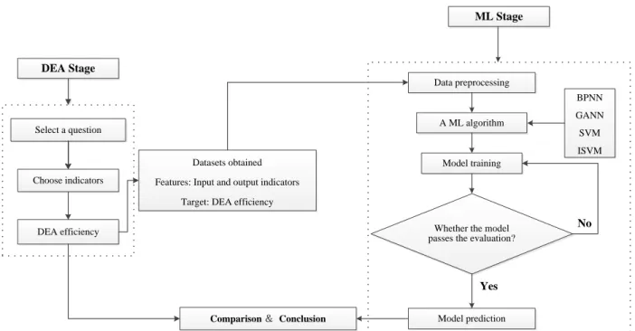
3 Research framework

The research framework on combining DEA method with four ML algorithms are discussed in the following: Four ML-DEA methods are used: DEA-CCR model (2.2) combined with BPNN (BPNN-DEA), with GA combined with BPNN (GANN-(BPNN-DEA), with SVM (SVM-(BPNN-DEA), and with ISVM (ISVM-DEA).

Firstly, the DEA-CCR model is used to measure the efficiency of each DMU in the training datasets, so that different DMUs can be “marked” by its technical efficiency (namely the DEA efficiency is target variable, and the input and output indicators of DEA model are feature variables); Then use ML algorithms to parse these DMUs marked by DEA efficiency, and learn the rules from them: What kind of input/output combination can be got the corresponding DEA efficiency? After training through the training datasets, the trained ML model is obtained until the model satisfies the evaluation standard, and then it is applied to “unmarked” DMUs which DEA efficiencies are unknown. Finally, the efficiency of them can be predicted through the trained ML model. Four discussed ML-DEA algorithms, i.e., BPNN-DEA, GANN-BPNN-DEA, SVM-BPNN-DEA, and ISVM-BPNN-DEA, are used to predict the DEA efficiency of new DMUs, respectively.

14 Select a question

Choose indicators

DEA efficiency

Datasets obtained Features: Input and output indicators

Target: DEA efficiency

Data preprocessing

A ML algorithm

Model training

Whether the model passes the evaluation?

Model prediction Yes No BPNN GANN SVM ISVM Comparison ＆ Conclusion DEA Stage ML Stage

Figure 4. Research framework of the linkage between DEA method and ML algorithms

The research framework consists of two main stages: the DEA stage and the ML stage, see Figure 4. In the first stage, i.e., DEA stage, according to actual problems, select DMUs with appropriate input and output indicators, and measure their DEA efficiencies by using a DEA model. In the second stage, i.e. ML stage, the DEA results are used as a basis for predicting the DEA efficiency of unmarked DMUs via frontier form learned by a selected ML algorithm. In ML stage, there are five steps:

Step 1: Data preprocessing. Mainly refers to data standardization processing.

Step 2: ML algorithms selection. Select one of four ML algorithms: BPNN, GANN, SVM, and ISVM algorithm, for training datasets.

Step 3: Model training. Use the training datasets with DMUs “marked” by its DEA efficiency to learn the rules from them, namely what kind of input/output combination can be got the corresponding DEA efficiency?

Step 4: Standard judgement. If the model satisfies the evaluation standard, namely the accuracy and stability of the model meet the requirements, then the trained ML model is obtained. Otherwise, continue training the model.

Step 5: Model prediction. The DEA efficiency of a new DMU can be predicted through the trained ML model. To predict efficiencies of the DMUs, we just need to add the new DMUs that needs to predict efficiency into the testing datasets, and running the MATLAB program, then the MATLAB software can automatically calculate its prediction efficiency.

15

In comparison & conclusion phase, the DEA efficiency needs to be analyzed, compared with ML-DEA efficiency (namely prediction efficiency), including the accuracy and stability of the model, statistical test and inference.

4 Empirical research and analysis

To illustrate the four ML-DEA algorithms discussed in this paper, i.e., BPNN-DEA, GANN-DEA, SVM-DEA, and ISVM-DEA. Where the BPNN and SVM are the classical algorithm, and the GANN is an integrated model that integrates the BPNN with the GA algorithm. The ISVM is adapted by adding a novel loop structure to search the best initial parameters of the model. More details about how the ISVM algorithm is adapted can be found in section 2.2.3 and the MATLAB code in Supplementary Material. The performances of Chinese manufacturing listed companies in 2016 are measured, predicted and compared with the efficiency scores obtained by the DEA-CCR model (2.2).

The data of 948 manufacturing companies (i.e. samples) in 2016 are collected from the Chinese Wind database, and the original data can be seen in Supplementary Material. Here, 900 samples are randomly chosen and used as the training datasets, and the other 48 samples are used as the testing datasets. These four ML algorithms run on the MATLAB software platform. Two inputs: owners’ equity and total operational expenses, and two outputs: operational income and net profit, are used to get the efficiency scores of the DEA-CCR model (2.2). The selection of input and output variables for the DEA-CCR model used in this paper is based on the existing literature on firm performance (e.g., Lin, et al., 2013).

Table 2. Correlation matrix

Equity Operational expenses Net profit Operational income

Equity 1

Operational expenses 0.896 1

Net profit 0.902 0.866 1

Operational income 0.899 1.000 0.875 1

Note:all coefficients are statistically significant at the 1% level (2-tail test).

Based on the correlation matrix shown in Table 2, it can be concluded that the property of isotonicity on the condition of using the DEA-CCR model (2.2) is satisfied. Table 2 shows that all coefficients are statistically significant at the 1% level (2-tail test), namely, there is a significant positive correlation between input and output indicators, so it is feasible to use the DEA method to measure the efficiency of DMUs.

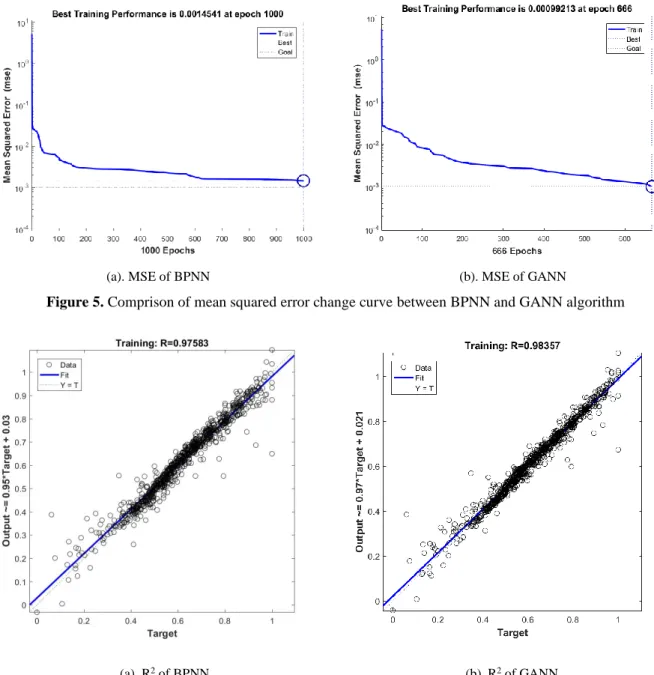
The plots in Figure 5 (a) show that the best training performance of BPNN algorithm is MSE = 0.0015 at the epoch 1000, the correlation coefficient (i.e. R2, the correlation coefficient is a numerical measure of some type of correlation, meaning a statistical relationship between two variables.) of the training datasets

16

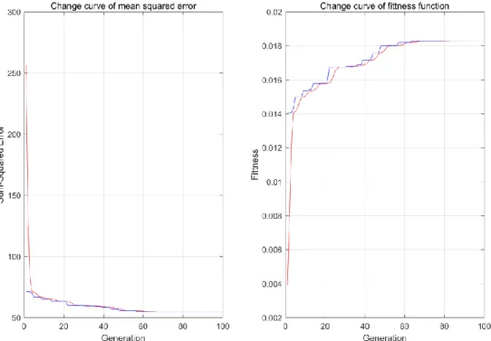
is R2_{= 0.9758 as shown in Figure 6 (a). After the optimization of GA, the best training performance of} GANN algorithm is MSE = 0.0010 at the epoch 666 as shown in Figure 5 (b), the R2 _{of training set is R}2 = 0.9836 as shown in Figure 6 (b), and the evolutionary process of GA is presented in Figure 7.

(a). MSE of BPNN (b). MSE of GANN

Figure 5. Comprison of mean squared error change curve between BPNN and GANN algorithm

(a). R2 _{of BPNN (b). R}2 _{of GANN}

Figure 6. Comprison of correlation coefficient between BPNN and GANN algorithms

As it can be seen from Figure 7, evolutionary process of GA shows that the MSE (MSE is a more convenient way to measure “average error”, and it can evaluate the degree of change of data) decreased gradually until it reaches a stable level, and the fitness of the population increased gradually until it reaches a stable level. After the optimization of GA, training speed of BPNN is faster (As it can be seen from Figure 5, it just need to iterate 666 epoch, the MSE drops below 0.001, but BPNN that has not been

17

optimized by GA needs to iterate 1000 epoch), the error is smaller, and the correlation is stronger (𝑀𝑆𝐸𝐺𝐴𝑁𝑁 = 0.0010 < 𝑀𝑆𝐸𝐵𝑃𝑁𝑁= 0.0015, 𝑅𝐺𝐴𝑁𝑁2 = 0.9836 > 𝑅𝐵𝑃𝑁𝑁2 = 0.9758, the smaller the MSE the smaller the error, the larger the R2 _{the stronger the correlation, R}2 _{refers to correlation coefficient that}

reflects the strength of the correlation between the two variables). Therefore, the performance of GANN algorithm is better than BPNN algorithm for training set.

Figure 7. Evolutionary process of GA

Table 3. A summary of DEA-CCR efficiency scores and predictied values of ML-DEA algorithms.

DEA-CCR BPNN-DEA GANN-DEA SVM-DEA ISVM-DEA

1 0.5211 0.5124 0.5261 0.6496 0.5777 2 0.7371 0.7369 0.7324 0.6554 0.7067 3 0.6247 0.6448 0.6436 0.6518 0.6361 4 0.7767 0.7614 0.7797 0.6606 0.7662 5 0.8119 0.8049 0.7981 0.6578 0.7515 6 0.8002 0.7816 0.8020 0.6667 0.8018 7 0.8083 0.8097 0.8060 0.6644 0.8023 8 0.7745 0.7753 0.7742 0.6612 0.7642 9 0.5407 0.5227 0.5298 0.6484 0.5685 10 0.7104 0.6718 0.6832 0.6551 0.6937 11 0.6266 0.6450 0.6409 0.6524 0.6433 12 0.9903 1.0192 1.0074 0.6713 0.9498 13 0.7803 0.8144 0.7806 0.7483 0.7852 14 0.6534 0.6738 0.6718 0.6535 0.6614 15 0.8900 0.8527 0.8482 0.6594 0.7865 16 0.8582 0.8328 0.8750 0.7095 0.8373 17 0.7223 0.7262 0.7235 0.6581 0.7176

18 18 0.6835 0.7014 0.6981 0.6550 0.6892 19 0.6347 0.6173 0.6234 0.6521 0.6334 20 0.8435 0.8275 0.8217 0.6588 0.7698 21 0.7810 0.7947 0.7924 0.6588 0.7571 22 0.8974 0.8732 0.8838 0.6782 0.9170 23 0.9504 0.9652 0.9703 0.6739 0.9753 24 0.6754 0.7001 0.6998 0.6545 0.6792 25 0.6888 0.7143 0.7109 0.6573 0.7037 26 0.6951 0.6947 0.6965 0.6547 0.6938 27 0.7216 0.7357 0.7312 0.6561 0.7086 28 0.9735 0.9152 0.9492 0.6951 1.1098 29 0.6051 0.6089 0.6075 0.6361 0.6207 30 0.8453 0.8603 0.8543 0.6617 0.8039 31 0.5210 0.5085 0.5117 0.6473 0.5523 32 0.5090 0.4555 0.5074 0.5904 0.5100 33 0.5476 0.5275 0.5307 0.6419 0.5240 34 0.7628 0.7795 0.7490 0.6826 0.7664 35 0.6751 0.7144 0.6949 0.6608 0.6749 36 0.5763 0.5889 0.5855 0.6497 0.5890 37 0.5696 0.5818 0.5798 0.6355 0.5726 38 0.7352 0.7350 0.7424 0.6645 0.7267 39 0.8304 0.8363 0.8287 0.8678 0.8350 40 1.0000 0.9604 1.0144 0.8388 0.9956 41 0.7148 0.7578 0.7319 0.6726 0.7104 42 0.8225 0.8075 0.8084 0.8180 0.8182 43 0.5664 0.6030 0.5820 0.5787 0.5709 44 0.7464 0.7714 0.7394 0.7002 0.7510 45 0.4962 0.4444 0.4868 0.5921 0.4769 46 0.8678 0.8283 0.8594 0.6916 0.8985 47 0.8568 0.8256 0.8571 0.6825 0.8781 48 0.3759 0.4549 0.4598 0.6478 0.5509 Mean 0.7249 0.7245 0.7277 0.6704 0.7274 STD 0.1408 0.2323 0.2352 0.1618 0.2278

Table 4. Common statistical parameters of four ML-DEA algorithms for testing datasets

Average accuracy MSE R2 Spearman’s Rho p-Value

BPNN-DEA 96.62% 0.0008 0.9758 0.988 p ≤ 0.001

GANN-DEA 97.93% 0.0004 0.9836 0.995 p ≤ 0.001

SVM-DEA 85.60% 0.0177 0.3094 0.866 p ≤ 0.001

ISVM-DEA 96.30% 0.0018 0.9113 0.983 p ≤ 0.001

The prediction DEA efficiency of the testing datasets is presented in Table 3, column 1 represents 48 test samples, column 2 represents the technical efficiency score, and column 3-6 represents the prediction efficiency of four ML algorithms, respectively. According to the results of Table 3, we can get the common statistical parameters of four ML-DEA algorithms for testing datasets which are shown in Table 4. Average accuracy is an important indicator that directly reflects the predictive power of a model. In this case study, the GANN-DEA algorithm has the highest accuracy, and the worst is the SVM-DEA algorithm. The results of Emrouznejad et al. (2009) showed that the NNDEA predictions for efficiency

19

score appeared to be a good estimate for the majority of cases, which is consistent with the finding of our work (Average accuracy of four ML-DEA is about 94%). What’s more, MSEGANN-DEA = 0.0004 <MSENN-DEA = 0.0008 <MSEISVM-DEA = 0.0018 <MSESVM-DEA = 0.0177, so the performance of the GANN-DEA algorithm is also the best, and the worst is the SVM-DEA algorithm, so the result is consistent with the advantage of GA algorithm mentioned above. As it can be seen from column 4, the size of R2 is ranked as follows:

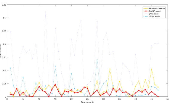
𝑹𝑮𝑨𝑵𝑵−𝑫𝑬𝑨𝟐 = 𝟎. 𝟗𝟖𝟑𝟔 > 𝑹𝑵𝑵−𝑫𝑬𝑨𝟐 = 𝟎. 𝟗𝟕𝟓𝟖 > 𝑹𝑰𝑺𝑽𝑴−𝑫𝑬𝑨𝟐 = 𝟎. 𝟗𝟏𝟏𝟑 > 𝑹𝑺𝑽𝑴−𝑫𝑬𝑨𝟐 = 𝟎. 𝟑𝟎𝟗𝟒 , so the correlation between prediction efficiency of GANN-DEA algorithm and DEA efficiency is the strongest, and the weakest is SVM-DEA algorithm. The results of Spearman’s Rho is given in column 5-6, all the correlations are significant at the 0.01 level (2-tail test). Hence the ranking order of the test samples between the DEA-CCR model and ML-DEA algorithms is very similar, it demonstrates that the idea of combining ML algorithms with the DEA method is reasonable. Figure 8 provides a visual comparison of the errors for four ML-DEA algorithms, it can be found that the comprehensive performance order of four ML-DEA algorithms ranked from good to poor is: GANN-DEA, BPNN-DEA, IDEA, and SVM-DEA.

Figure 8. Comparison of relativeerror of 4 ML-DEA algorithms 5 Conclusions and direction for future reserach

Following the previous studies, this paper aims to establish a linkage between the DEA method and ML algorithms, and proposes an alternative way that combines DEA with ML algorithms to predict the DEA efficiency of new DMUs. Four ML-DEA algorithms are discussed, namely, DEA-CCR model combined with back-propagation neural network (BPNN-DEA), with genetic algorithm (GA) integrated with and

20

back-propagation neural network (GANN-DEA), with support vector machines (SVM-DEA), and with improved support vector machines (ISVM-DEA), respectively. For the purpose of this study, this paper uses the DEA-CCR efficiency results trying to predict efficiency on a new DMUs by training datasets and by predicting the shape of the efficiency frontier.

As different algorithms have different performance effects, choosing an appropriate ML algorithm is of great significance for improving the accuracy of prediction. By selecting different models or models integration, selecting different datasets or adjusting the size of the datasets, after a large number of actual tests, the most suitable algorithm can be found.

To illustrate the method of the paper, a real dataset of Chinese manufacturing listed companies in 2016 is collected, analyzed and compared with the efficiency scores obtained by the DEA-CCR model. The empirical result shows that the average accuracy of the predicted efficiency of DMUs is about 94%, and the comprehensive performance order of four ML-DEA algorithms ranked from good to poor is GANN-DEA, BPNN-GANN-DEA, ISVM-GANN-DEA, and SVM-DEA.

The future research direction is to collect larger real datasets, integrating and optimizing more DEA methods combined with ML algorithms for predicting DEA efficiency of DMUs, comparing the computational complexity of ML-DEA and DEA methods at the same time. On the other hand, there are also some technical issues that need further study, such as the selection of activation function, optimization algorithm, cross-validation design and regression model selection, etc.

Conflicts of Interest: The authors claim no conflicts of interest, and manuscript is approved by all authors for publication.

Acknowledgments: The authors would like to thank to the peers for their insightful comments and suggestions in DEA 40th Anniversary - International Conference of Data Envelopment Analysis, as results the paper has been improved substantially. Meanwhile, this paper has been funded by the Fundamental Research Funds for the Central Universities (Grant Nos. 331510004007000002).

Data Availability Statement: The data of Chinese manufacturing listed companies used to support the findings of this study are included within the Supplementary Materials.

References

Banker, R. D., Charnes, A., & Cooper, W. W. (1984). Some models for estimating technical and scale inefficiencies in Data Envelopment Analysis. Management Science, 30:1078-1092.

21

Barros, C. P., & Wanke, P. (2014). Insurance companies in Mozambique: A two-stage DEA and neural networks on efficiency and capacity slacks. Applied Economics, 46 (29): 3591-3600.

Ben-Hur, A., Horn, D., Siegelmann, H., & Vapnik, V. N. (2001). Support vector clustering. Journal of Machine Learning Research, 2: 125-137.

Bishop, C. M. (2006). Pattern Recognition and Machine Learning, Springer, ISBN 978-0-387-31073-2. Brunetti, A., Buongiorno, D., Trotta, G. F., & Bevilacqua, V. (2018). Computer vision and deep learning techniques for pedestrian detection and tracking: A survey. Neurocomputing, 300: 17-33.

Campbell, C., & Ying, Y. (2011). Learning with Support Vector Machines. Morgan and Claypool.

Charnes, A., Cooper, W. W., & Rhodes, E. (1978). Measuring the efficiency of decision-making units.

European Journal of Operational Research, 2 (6): 429-444.

Cheng, C. S. (1995). A multi-layer neural network model for detecting changes in the process mean.

Computers & Industrial Engineering, 28 (1): 51-61.

Chen, Y., Yang, J., Wang, C., & Liu, N. (2016). Multimodal biometrics recognition based on local fusion visual features and variational Bayesian extreme learning machine. Expert Systems with Applications, 64: 93-103.

Cooper, W. W., Seiford, L. M., & Zhu, J. (2004). Handbook on data envelopmentanalysis, Kluwer Academic.

Cortes, C., & Vapnik, V. N. (1995). Support-vector networks. Machine Learning, 20 (3): 273–297. De Clercq, D., Wen, Z., & Fei, F. (2019). Determinants of efficiency in anaerobic bio-waste co-digestion facilities: A data envelopment analysis and gradient boosting approach. Applied Energy, 253, 113570. Drucker, H., Burges, C. J., Kaufman, L., Smola, A., & Vapnik, V. N. (1997). Support Vector Regression Machines. Advances in Neural Information Processing Systems, 9: 155-161.

Emrouznejad, A. (2005). Measurement efficiency and productivity in SAS/OR. Journal of Computers and Operation Research, 32 (7): 1665-1683.

Emrouznejad, A., & Shale, E. (2009). A combined neural network and DEA for measuring efficiency of large scale datasets. Computers & Industrial Engineering, 56: 249-254.

Emrouznejad, A., & Yang, G. (2018), A survey and analysis of the first 40 years of scholarly literature in DEA: 1978-2016. Journal ofSocio-Economic Planning Sciences, 61 (1): 1-5.

22

Fallahpour, A., Olugu, E. U., Musa, S. N., Khezrimotlagh, D., & Wong, K. Y. (2016). An integrated model for green supplier selection under fuzzy environment: application of data envelopment analysis and genetic programming approach. Neural Computing and Applications, 27 (3): 707-725.

Farrell, M. J. (1957). The measurement of productive efficiency. Journal of the Royal Statistical Society, 120 (3): 253-281.

Fethi, M. D. & Pasiouras, F. (2010). Assessing bank efficiency and performance with operational research andartificial intelligence techniques: A survey. EuropeanJournal of Operational Research, 204: 189-198. Gunn, S. (1998). Support vector machines classification and regression. ISIS Technical Report, Image Speech  Intelligent Systems Group, University of Southampton.

Gupta, A., Kohli, M., & Malhotra, N. (2016, July). Classification based on Data Envelopment Analysis and supervised learning: A case study on the energy performance of residential buildings. 2016 IEEE 1st international conference on power electronics, intelligent control and energy systems (ICPEICES) (pp. 1-5). IEEE.

Hebb, D. O. (1949). The Organization of Behavior: A Neurapsychological Theory. Wiley, New York. Holland, J. H. (1975). Adaptation in natural and artificial Systems: an introductory analysis with applications to biology, control, and artificial intelligence, University of Michigan Press, Ann Arbor. Jiang, B., Chen, W., Zhang, H., & Pan, W. (2013). Supplier’s efficiency and performance evaluation using DEA-SVM approach. Journal of Software, 8 (1): 25-30.

Kavakiotis, I., Tsave, T., Salifoglou, A., Maglaveras, N., Vlahavas, I., & Chouvarda, I. (2017).Machine Learning and Data Mining Methods in Diabetes Research. Computational and Structural Biotechnology Journal, 15, 104-116.

Kitano, H. (1990). Designing Neural Networks Using Genetic Algorithms with Graph Generation Systems. Complex Systems, 4: 461-476.

Kwok, J. Tin-Yau. (1998). Support vector Mixture for classification and regression problems. Proceeding of 14th international conference on pattern recognition, Brisbane, Australia, 1: 255-258.

Kwon, H. B., & Lee, J. (2015). Two-stage production modeling of large US banks: A DEA-neural network approach. Expert Systems with Applications, 42 (19): 6758-6766.

Lin, T.Y., & Chiu, S. H. (2013). Using independent component analysis and network DEA to improve bank performance evaluation. Economic Modelling, 32: 608–16.

23

Liu, H., Chen, T., Chiu, Y., & Kuo, F. (2013). A Comparison of Three-Stage DEA and Artificial Neural Network on the Operational Efficiency of Semi-Conductor Firms in Taiwan. ModernEconomy, 4: 20-31. Lee, T. K., Cho, J. H., Kwon, D. S., & Sohn, S. Y. (2019). Global stock market investment strategies based on financial network indicators using machine learning techniques. Expert Systems with Applications, 117: 228-242.

Liu, L. & Zhang X. (2019). Analysis of Financing Efficiency of Chinese Agricultural Listed Companies Based on Machine Learning. Complexity, vol. 2019, Article ID 9190273, 11 pages.

Mcculloch,W. S., & Pitts, W. (1943). A Logical Calculus of the IdeasImmanent in Nervous Activity.

Bulletin of Mathematical Biophysics, 5 (4): 115-133.

Mehryar, M., Afshin, R., & Ameet, T. (2012). Foundations of Machine Learning. The MIT Press.

Misiunas, N., Oztekin A., Chen Y., & Chandra, K. (2016). DEANN: A healthcare analytic methodology of data envelopment analysis and artificial neural networks for the prediction of organ recipient functional status. Omega, 58: 46-54.

Mulwa, R., Emrouznejad, A., & Muhammad, L. (2008). Economic Efficiency of small holder maize producers in Western Kenya: a DEA meta-frontier analysis. International Journal of Operational Research, 4 (3): 250-267.

Nandy, A., & Singh, P. K. (2020, In Press). Farm efficiency estimation using a hybrid approach of machine-learning and data envelopment analysis: evidence from rural eastern india. Journal of Cleaner Production.

Rattay, F. (1999). The basic mechanism for the electrical stimulation of the nervous system. Neuroscience, 89 (2): 335-346.

Ray, S. C., & Das, A. (2010). Distribution of cost and profit efficiency: Evidence from Indian banking.

European Journal of Operational Research, 201 (1): 297-307.

Rebai, S., Ben Yahia, F., & Essid, H. (2020, In Press). A graphically based machine learning approach to predict secondary schools performance in Tunisia. Socio-Economic Planning Sciences.

Rosenblatt, F. (1958). The perceptron: a probabilistic model for information storage and organization in the brain. Psychological Review, 65 (6): 386-408.

Rumelhart, D. E., & Mcclelland, J. L. (1986). Parallel distributed processing: explorations in the microstructure of cognition, Foundations of Research, MIT Press, Cambridge (Massachusetts).

24

Rumelhart, D. E., Hinton, G. E. & Williams, R. J. (1986). Learning representations by back-propagating errors. Nature, 323 (6088): 533-536.

Schmitt, L. M. (2001). Theory of Genetic Algorithms. Theoretical Computer Science, 259, 1–61. Schapire, R. (1990). The strength of weak learnability. Machine Learning, 5 (1): 197–227.

Smola, A. J., & Schölkopf, B. (2004). A tutorial on support vector regression. Statistics and Computing, 14 (3): 199-222.

Song, Y., Yang, G., Yang, J., Khoveyni, M. & Xu D. (2018). Using Two-layer Minimax Optimization and DEA to Determine Attribute Weights. Journal of Management Science and Engineering, 3 (2): 76-100.

Steinwart, I., & Christmann, A. (2008). Support Vector Machines. Springer-Verlag, New York.

Stuart, J. R. & Peter, N. (2010). Artificial Intelligence: A Modern Approach. Third Edition, Prentice Hall. Turing, A. M. (1950). Computing machinery and intelligence. Mind, 59: 433-460.

Vapnik, V. N. (1993).Three fundamental concepts of the capacity of learning machines. Physica A: Statistical Mechanics and its Applications, 200: 538-544.

Vapnik, V. N., Golowich, S. & Smola, A. (1997). Support vector method for function approximation, regression estimation, and signal processing. Advances in Neural Information Processing Systems, 9: 281-287.

Vose, M. D. (1999). The Simple Genetic Algorithm: Foundations and Theory. Cambridge, MA: MIT Press.

Werbos, P. J. (1981). Applications of advances in nonlinear sensitivity analysis. In Proceedings of the 10th IFIP Conference, NYC, 31.8-4.9: 762-770.

Wikipedia (2019), Machine learning:https://en.wikipedia.org/wiki/Machine_learning.

Xu, Y., Yang, C., Zhong, J., Wang, N. & Zhao, L. (2018). Robot teaching by teleoperation based on visual interaction and extreme learning machine. Neurocomputing, 275: 2093-2103.

Yang, L. H., Wang, Y. M., Lan, Y. X., Chen, L., & Fu, Y. G. (2017). A data envelopment analysis (DEA)-based method for rule reduction in extended belief-rule-based systems. Knowledge-Based Systems, 123: 174-187.

25

Yang, G., Ren, X., Khoveyni, M., & Eslami, R. (2020, In Press).Directional congestion in the framework of data envelopment analysis.Journal of Management Science and Engineering.

Zhang, M. (2017). The number of small and micro-sized enterprises in China has exceeded 73 million,