Optical Design Document
Prepared by: Name:
Rodolfo Canestrari
Signature: Date: 09-‐11-‐2012INAF-‐OABr
Reviewed by: Name:
Gabriele Rodeghiero
Signature: Date: 09-‐11-‐2012
INAF-‐OAPd
Approved by: Name:
Mauro Fiorini
Signature: Date:
Luca Stringhetti
Enrico Giro
TABLE OF CONTENTS
DISTRIBUTION LIST ... 4
DOCUMENT HISTORY ... 5
LIST OF ACRONYMS ... 6
APPLICABLE DOCUMENTS ... 6
REFERENCE DOCUMENTS ... 6
1.
PREFACE ... 7
2.
INTRODUCTION ... 8
3.
THE OPTICAL LAYOUT ... 10
3.1
Obscuration from the detector ... 13
4.
THE OPTICAL SURFACES ... 15
4.1
The primary mirror, M1 ... 15
4.2
The secondary mirror, M2 ... 17
5.
THE DETECTOR ASSEMBLY ... 18
6. OPTICAL ERROR BUDGET TREE ... 21
6.1
Definitions ... 21
6.1.1
Reference system ... 21
6.1.2
Sensitivity ... 22
6.2
Error budget tree related to M1 ... 22
6.3
Error budget tree related to M2 ... 23
6.3.1
Profile errors ... 23
6.3.2
Alignment errors ... 23
6.4
Surface microroughness ... 25
6.5
Error budget tree related to CAM ... 25
6.5.1
Profile errors ... 25
6.5.2
Alignment errors ... 25
7.
FEATURED ENHANCEMENTS ... 26
7.1
Reimaging system ... 26
7.3
Baffle ... 30
DOCUMENT HISTORY
Version Date Modification
1.0 30-‐06-‐2012 first version
1.1 09-‐11-‐2012 Minor updates and proof reading
LIST OF ACRONYMS
CTA Cherenkov Telescope Array DET Detector
EC Elemental Cell M1 Primary Mirror M2 Secondary Mirror
PDM Photon Detection Module SST Small Size Telescope UNIT Basic detector unit
APPLICABLE DOCUMENTS
[AD1] CTA-‐TC_PR1-‐110331 “Level A: Preliminary CTA System Performance Requirements”
REFERENCE DOCUMENTS
[RD1] ASTRI-‐IR-‐OAB-‐3100-‐009 “The optical layout of the ASTRI prototype: 4 meter
Schwarzschild-‐Couder Cherenkov telescope for CTA with 10° of field of view”
[RD2] ASTRI-‐SPEC-‐OAB-‐3100-‐002 “Error Budget Tree for the ASTRI prototype: Structure
and Mirrors”
[RD3] ASTRI-‐TN-‐IASFPA-‐3200-‐015 “Effects of the focal plane lodging for the SST-‐2M
single prototype (Versione 1.0)”
[RD4] ASTRI-‐TN-‐IASFPA-‐3200-‐016 “Stray-‐light study for the SST-‐2M single prototype
(Versione 1.0)”
1.
PREFACE
This document describes the optical design as reported in [RD1] for a wide field, aplanatic, double-‐reflection Cherenkov telescope of 4 meters class. Updates and additional paragraphs are also provided such as 3.1 Obscuration from the detector.
Moreover, the former chapter 5 Tolerances of [RD1] is now replaced by a more extensive discussion of the optical error budget adopted to design the ASTRI telescope and mirrors as reported in [RD2].
2.
INTRODUCTION
This design is developed by INAF in the framework of the ASTRI project and it will be implemented into the end-‐to-‐end prototype to be developed. The proposed layout intends to be fully compliant with the requirements for the telescopes composing the SST array of the CTA Observatory Errore. L'origine riferimento non è stata trovata..
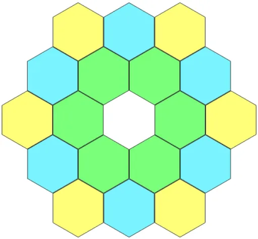
The design hereafter presented is done taking into account both the segmentation of the primary mirror M1 shown in Figure 2.1 and the arrangement of detection units into the detector DET as shown in Figure 2.2 (a description of the detector arrangement and nomenclature is postponed in 5).
Figure 2.1 Tessellation of the primary mirror M1.
Figure 2.2 Arrangement of the detector units on the curved focal plane. In transparency a protective window with no optical power is visible.
The design optimization has been done in such a way the amount of energy contained within 2x2 physical pixels, hereafter called Cherenkov pixel, is not less than 80% along the entire field angle. This parameter is named Ensquared Energy.
The design has been performed using the commercial software for optical system design ZEMAX.
3.
THE OPTICAL LAYOUT
The optical system is a Schwarzschild-‐Couder configuration with a focal ratio F# of 0.5, see Figure 3.1. The design has plate scale of 37.5 mm/°, the Cherenkov pixel is approximately 0.16°, over an equivalent focal length of 2150 mm. This delivers a usable field of view up to 9.6° in diameter.
Figure 3.1 The Schwarzschild-‐Couder optical design adopted for ASTRI.
The images of a point source placed 10 km above the telescope are also shown. Figure 3.2 is a series of six zooms of the entire detector down to the Cherenkov pixel for the field angles: 0°, 1°, 2°, 3°, 4° and 4.8°. From these images have been evaluated the ensquared energies curves plotted in Figure 3.3.
Figure 3.2 Images for 0°, 1°, 2°, 3°, 4° and 4.8° of field angle of a point source located 10 km above the telescope. The images are oversampled because each box has the same dimensions
of a Cherenkov pixel.
Figure 3.3 Ensquared energy for various field angles.
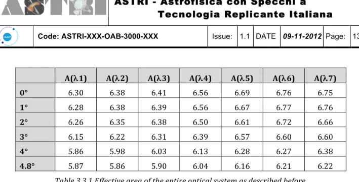
Concerning the throughput we give the effective area, expressed in squared meters, of the entire optical system taking into account:
-‐
segmentation of the primary mirror;
-‐
obscuration of the secondary mirror;
-‐
obscuration of the detector;
-‐
reflectivity of M1 and M2 (standard coated, mean reflectivity 90%) as
function of the energy and incident angle;
-‐
a protection window for the detector (standard coated, transmission >
98%);
-‐
efficiency of the detector as function of the incident angles (ranging from
25° to 72°).
The values in Table 3.3.1 do not consider the quantum efficiency of the detector and the absorption from the atmosphere, whilst they are calculated as function of the incoming wavelengths (λ1=320nm; λ2=350nm; λ3=400nm; λ4=450nm; λ5=500nm; λ6=550nm; λ7=600nm) for different field angles.
To complete the optical design description we report also the temporal behavior of the optics. Figure 3.4 shows that the system is isochronous down to 3x10-‐12 s.
A(λ1) A(λ2) A(λ3) A(λ4) A(λ5) A(λ6) A(λ7) 0° 6.30 6.38 6.41 6.56 6.69 6.76 6.75 1° 6.28 6.38 6.39 6.56 6.67 6.77 6.76 2° 6.26 6.35 6.38 6.50 6.61 6.72 6.66 3° 6.15 6.22 6.31 6.39 6.57 6.60 6.60 4° 5.86 5.98 6.03 6.13 6.28 6.27 6.38 4.8° 5.87 5.86 5.90 6.04 6.16 6.21 6.22
Table 3.3.1 Effective area of the entire optical system as described before.
Figure 3.4 Temporal behavior of the optical system.
3.1
Obscuration from the detector
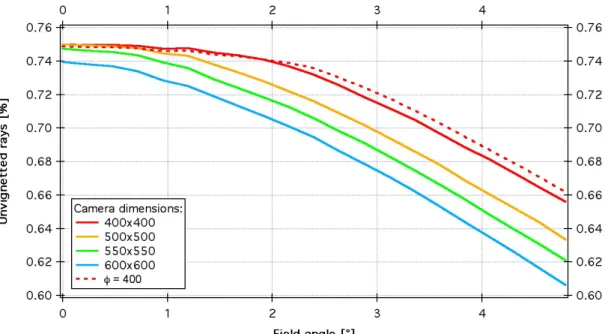
As mentioned before, the throughput given in Table 3.3.1 takes into account also the loss coming from the detector size. The dimensions considered in the computation are those of the ideal detector, i.e. nominal dimensions to use the full field of view. However, we have
analyzed the influence of a real detector by changing its front dimensions. In Figure 3.5 we report the vignetting induced by the detector as function of the field of view.
Further studies that consider the influence of the bottom side of the detector are reported in [RD3]. Absent or very limited variation of the telescope efficiency is observed.
Figure 3.5 Fraction of incident rays arriving on the detector as a function of the field angle for varius detector’s dimensions.
4.
THE OPTICAL SURFACES
The mirror surfaces can be described with the following polynomial equation:
where z is the surface profile, r the surface radial coordinate, c the curvature (the reciprocal of the radius of curvature), k the conical constant, αi the coefficients of the
asphere.
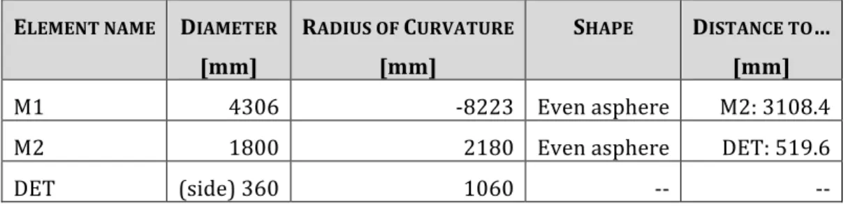
The main system dimensions are listed in Table 4.4.1. Figure 4.1 and Figure 4.2 show the sags as a function of the surface radial coordinate for M1 and M2 respectively.
ELEMENT NAME DIAMETER
[mm]
RADIUS OF CURVATURE
[mm]
SHAPE DISTANCE TO…
[mm]
M1 4306 -‐8223 Even asphere M2: 3108.4
M2 1800 2180 Even asphere DET: 519.6
DET (side) 360 1060 -‐-‐ -‐-‐
Table 4.4.1 Optical system main dimensions.
4.1
The primary mirror, M1
The primary mirror is segmented following the scheme reported in Figure 2.1. The full reflector is composed of 18 segments (the central one is not used). The segmentation requires three types of segments having different surface profiles:
-‐ the green segments, inner corona: M1a; -‐ the light blue segments, central corona: M1b; -‐ the yellow segments, outer corona: M1c.
The segments have hexagonal shape with aperture equal to 849 mm from face to face. Each segment has 9 mm of gap from the neighbours for mounting and alignment purposes. Each segment will be equipped with two actuators plus one fixed point for alignment. Only tilt misplacements will be corrected; piston correction will not be available for the primary mirror segments.
Adopting the same mathematical notation introduced before we report in Table 4.4.2 the description of the surface profile of M1.
COEFFICIENT M1 α1 0.00 α2 9.61060e-‐013 α3 -‐5.65501e-‐020 α4 6.77984e-‐027 α5 3.89558e-‐033 α6 5.28038e-‐040 α7 -‐2.99107e-‐047 α8 -‐4.39153e-‐053 α9 -‐6.17433e-‐060 α10 2.73586e-‐066
Table 4.4.2 Coefficients describing the aspherical terms in M1.
Figure 4.1 Profile of M1 as function of the radial coordinate.
4.2
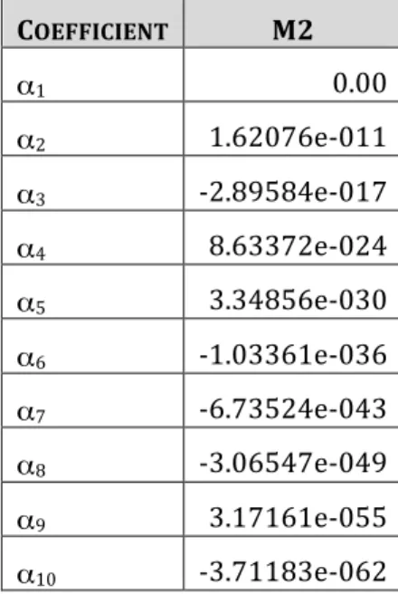
The secondary mirror, M2
The secondary mirror is monolithic and equipped with three actuators. The implementation of the third actuator makes available also the piston/focus adjustment for the entire optical system.
Adopting the same mathematical notation introduced before we report in Table 4.3 the description of the surface profile of M2.
COEFFICIENT M2 α1 0.00 α2 1.62076e-‐011 α3 -‐2.89584e-‐017 α4 8.63372e-‐024 α5 3.34856e-‐030 α6 -‐1.03361e-‐036 α7 -‐6.73524e-‐043 α8 -‐3.06547e-‐049 α9 3.17161e-‐055 α10 -‐3.71183e-‐062
Table 4.3 Coefficients describing the aspherical terms in M2.
5.
THE DETECTOR ASSEMBLY
The detector is based on Silicon Photon Multiplier devices made up of APDs operated in Geiger mode. The design presented in this document makes use of devices available on the market and their arrangement is one constrain adopted for the trade-‐off.
Figure 5.1 shows the basic units and the way in which we intend to assemble them together:
-‐ The UNIT is the primary monolithic device; it is composed of 4x4 pixels of 3 mm in side. A group of 2x2 pixels forms the Cherenkov pixel.
-‐ The ELEMENTAL CELL EC is a symmetric assembly of 2x2 UNITs mounted on a PCB.
-‐ The PHOTON DETECTION MODULE PDM is made up by 2x2 ECs for a total number of 256 pixels; it maintains a symmetry top-‐bottom and left-‐right; it is the basic detection unit to be mechanically integrated into the camera body. Over the geometrical area covered by one PDM, the dead area is about 31.5%.
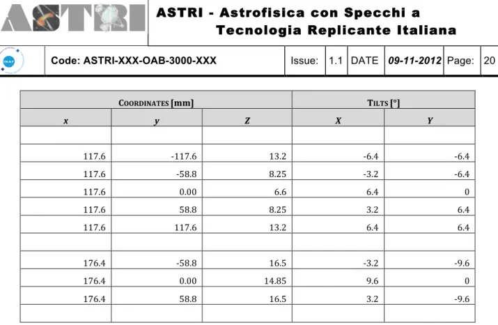
This optical design delivers up to 9.6° of corrected field of view corresponding to a grid of 7x7 PDMs. The field of view can be filled with 31 PDMs (25 + 12 half PDMs) arranged as shown in
Figure 2.2
, the grand total of Cherenkov pixels will be 1984. InTable 5.1
are listed the (x, y, z) coordinates of the centers of each PDM and their (x, y) tilts.
Figure 5.1 Adopted nomenclatures of SiPM detector units.
COORDINATES [mm] TILTS [°] x y z x y -‐176.4 -‐58.8 16.5 -‐3.2 9.6 -‐176.4 0.00 14.85 -‐9.6 0 -‐176.4 58.8 16.5 3.2 9.6 -‐117.6 -‐117.6 13.2 -‐6.4 6.4 -‐117.6 -‐58.8 8.25 -‐3.2 6.4 -‐117.6 0.00 6.6 -‐6.4 0 -‐117.6 58.8 8.25 3.2 6.4 -‐117.6 117.6 13.2 6.4 6.4 -‐58.8 -‐176.4 16.5 -‐9.6 3.2 -‐58.8 -‐117.6 8.25 -‐6.4 3.2 -‐58.8 -‐58.8 3.35 -‐3.2 3.2 -‐58.8 0.00 1.7 -‐3.2 0 -‐58.8 58.8 3.35 3.2 3.2 -‐58.8 117.6 8.25 6.4 3.2 -‐58.8 176.4 16.5 9.6 3.2 0.00 -‐176.4 14.85 0 -‐9.6 0.00 -‐-‐117.6 6.6 0 -‐6.4 0.00 -‐58.8 1.7 0 -‐3.2 0.00 0.00 0.00 0 0 0.00 58.8 1.7 0 3.2 0.00 117.6 6.6 0 6.4 0.00 176.4 14.85 0 9.6 58.8 -‐176.4 16.5 -‐9.6 -‐3.2 58.8 -‐117.6 8.25 -‐6.4 -‐3.2 58.8 -‐58.8 3.35 -‐3.2 -‐3.2 58.8 0.00 1.7 3.2 0 58.8 58.8 3.35 3.2 -‐3.2 58.8 117.6 8.25 6.4 -‐3.2 58.8 176.4 16.5 9.6 -‐3.2
COORDINATES [mm] TILTS [°] x y Z X Y 117.6 -‐117.6 13.2 -‐6.4 -‐6.4 117.6 -‐58.8 8.25 -‐3.2 -‐6.4 117.6 0.00 6.6 6.4 0 117.6 58.8 8.25 3.2 6.4 117.6 117.6 13.2 6.4 6.4 176.4 -‐58.8 16.5 -‐3.2 -‐9.6 176.4 0.00 14.85 9.6 0 176.4 58.8 16.5 3.2 -‐9.6
Table 5.1 Coordinates and tilts of the PMDs composing the detector assembly in a reference frame centered on the focal plane (z axis pointing toward M1).
6.
OPTICAL ERROR BUDGET TREE
6.1
Definitions
6.1.1 Reference system
The reference system is defined as in Figure 6.1, if not explicitly stated. The z axis is the optical axis and it points toward the M2.
Figure 6.1 Reference system definition and segments’ numbering.
According to the M1 segments’ numbering, we give in Table 6.1 the nominal position of the centers of each hexagon. The numbers are in mm unit.
The segments numbered 1, 8 and 13 are used as reference and they correspond to the color index green, light blue and yellow respectively.
6.1.2 Sensitivity
As described in [RD1] the optical layout of the ASTRI prototype has the energy concentration (ensquared energy) greater then 80% into the Cherenkov pixels along the entire field of view.
This definition is meaningful taking into account the entire telescope optical design and is not referred to the single mirror segments, like in the Davies-‐Cotton case. Considering this fact the Error Budget Tree hereafter described can be compiled in such a way the global effect of all contributions keeps the energy concentration (ensquared energy) better then (or equal to) 70%.
This can be translated in a PV error budget equal to 120 µm and slope error budget equal
to 60’’ rms.
6.2
Error budget tree related to M1
Let’s consider the secondary mirror M2 being monolithic, infinitely rigid and having the nominal profile.
Value Units Comments
1. M1 segments profile errors 1.1. Manufacturing a. Mold 30 10 -‐-‐ -‐-‐ µm PV ‘‘ rms
It comes from FLABEG, no/very poor control on it.
The rms is sampled at least with a grid of 25 mm of pitch. b. Replication process 50 10 -‐-‐ -‐-‐ µm PV ‘‘ rms
It comes from FLABEG, limited control on it.
The rms is sampled at least with a grid of 25 mm of pitch.
c. Glass cutting -‐-‐ 6 ‘ Axial (normal to the surface on the hexagon center) rotation of the glass profile wrt the nominal one.
It is equivalent to 0.87 mm over the length of the hexagonal side.
d. Integration TBD TBD -‐-‐ -‐-‐ µm PV ‘‘ rms
Contribution of the cold shaping step (could be also improvements)
SUBTOTAL 58 -‐-‐ -‐-‐ 6 µm PV ‘ Quadratic propagation 1.2. Structural a. Mounting 40 2 mm PV ‘‘ rms
Contribution of the mounting supports (e.g. gluing of the interfaces, …) The shape will be modified only locally.
b. Gravity 30 TBC
µm PV ‘‘ rms
Contribution of the normal gravity
c. Operative wind 30 TBC
µm PV ‘‘ rms
Contribution of the operative wind
d. Operative temp. 1 µm PV Homogeneous temperature shift up to ±20°C
SUB TOTAL 58 µm PV Quadratic propagation
GRAND TOTAL 82 µm PV Error budget in quadratic
propagation.
2. M1 segments alignment errors 2.1 Translations
a. x ±2 mm These values are referred to the positions of the centers of the hexagons as reported in Table 1.
b. y ±2 mm
c. z ±4 mm
2.2 Rotations
a. z’ ±4 ‘ z’ is defined as the axis parallel to the z (optical axis) passing through the center of the hexagons.
2.3 Tilts
a. x ±30 ‘‘
b. y ±30 ‘‘
Table 6.2 Error budget tree for M1.
Not appreciable degradation (i.e. <5%) of the ensquared energy is reported within the values of Table 6.2. There is no need to actively correct with actuators within these ranges. However, these values shall be used to define the accuracy and the range of the actuators.
6.3
Error budget tree related to M2
6.3.1 Profile errors
Let’s consider now the M1 segments being perfectly aligned, infinitely rigid (both the mirrors themselves and the telescope structure) and having the nominal profile.
We consider now the contributions coming from a not perfect secondary mirror.
6.3.2 Alignment errors
The positioning errors along (x, y) and the relative tilts translate almost completely in pointing errors of the telescope (the contribution to the ensquared energy is negligible). The error along z is a defocusing of the telescope and can be correct adjusting the 3 actuators of M2.
Value Units Comments 3. M2 profile errors 3.1. Manufacturing a. Mold 120 40 µm PV ’’ rms
It comes from FLABEG, no/very poor control on it.
The rms is sampled at least with a grid of 25 mm of pitch. b. Replication process 200 40 µm PV ’’ rms
It comes from FLABEG, limited control on it.
The rms is sampled at least with a grid of 25 mm of pitch.
c. Glass cutting n.a. ‘ Axial (normal to the surface on the hexagon center) rotation of the glass profile wrt the nominal one.
d. Integration TBD TBD
µm PV ‘’ rms
Contribution of the cold shaping step (could be also improvements)
SUBTOTAL 217
(54)
µm PV
µm PV
Quadratic propagation
(calculated taking into account the demagnification factor, equal to 4)
3.2. Structural a. Mounting 40 2 µm PV ‘‘ rms
Contribution of the mounting supports (e.g. gluing of the interfaces, …) The shape will be modified only locally.
b. Gravity 120
TBC
µm PV ‘‘ rms
Contribution of the normal gravity
c. Operative wind 120 TBC
µm PV ‘‘ rms
Contribution of the operative wind
d. Operative temp. 4 µm PV Homogeneous temperature shift up to ±20°C SUBTOTAL 174 (44) µm PV µm PV Quadratic propagation
(calculated taking into account the demagnification factor, equal to 4)
GRAND TOTAL 278 (69) µm PV µm PV
Error budget in quadratic propagation.
(calculated taking into account the demagnification factor, equal to 4)
4. M2 alignment errors
4.1 Translations
a. x ±3 mm This introduces pointing errors to be modeled with T-‐points. (1 mm = 38’’ pointing error) b. y ±3 mm c. z ±4 ±1 mm mm Relative to M1 Relative to DET 4.2 Rotations
4.3 Tilts
a. x
10 ‘ The tilts do not constrain the design of the telescope structure up to the indicated value.
Obliviously, this introduces pointing errors to be modeled with T-‐points.
b. y 10 ‘
Table 6.3 Error budget tree for M2.
6.4
Surface microroughness
Concerning the microroughness, it scatters the light causing the blurring of the PSF and the increase of the background light on adjacent pixels. The microroughness is evaluated for spatial frequencies below the millimeter scale; the maximum tolerable value is 4-‐5 nm rms.
6.5
Error budget tree related to CAM
6.5.1 Profile errors
Let’s consider now the M1 segments and M2 monolithic mirror perfectly aligned, infinitely rigid (both the mirrors themselves and the telescope structure) and having the nominal profile.
We consider now the contributions coming from a not perfect camera mounting.
6.5.2 Alignment errors
The positioning errors along (x, y) translate almost completely in pointing errors of the telescope (the contribution to the ensquared energy is negligible). Nevertheless, we fix the maximum displacements to ±5.5 mm along each axis (x, y).
Tilts errors along (x, y) of the order of 20 arcmin for each axes can be tolerable.
The error along z is a defocusing of the telescope and is correct adjusting the 3 actuators of M2.
7.
FEATURED ENHANCEMENTS
The optical design and its performances as they are depicted in the previous sections of this document shall to be considered the baseline choice for the ASTRI prototype. It can be implemented exactly as described before; we call it naked configuration, i.e. without requiring any particular technological development (apart from the obvious work needed for the mirrors and detector implementations). The naked configuration provides a sort of minimum performances at the minimum cost; performances that are in any case already compliant with the main needs of CTA.
In this section, some enhancements are described in order to push these performances. These enhancements can be effective only subsequently to their technological developments. Table 7.1 shows the ideal effective area achievable in case of total reflection or transmission of the optical components.
A(λ1) A(λ2) A(λ3) A(λ4) A(λ5) A(λ6) A(λ7) 0° 6.55 7.24 7.38 7.46 7.46 7.35 7.08 1° 6.53 7.24 7.36 7.46 7.44 7.36 7.09 2° 6.51 7.20 7.35 7.39 7.37 7.31 7.00 3° 6.40 7.05 7.27 7.28 7.33 7.18 6.93 4° 6.09 6.79 6.95 6.97 7.00 6.82 6.70 4.8° 6.10 6.65 6.80 6.87 6.98 6.75 6.53
Table 7.1 Effective area of the optical system equipped with the described enhancements.
7.1
Reimaging system
The reimaging system has the aim to recover the losses caused by photons that go into the detector dead area. Depending from its implementation, it will be possible to recover up to the 70% of photons losses.
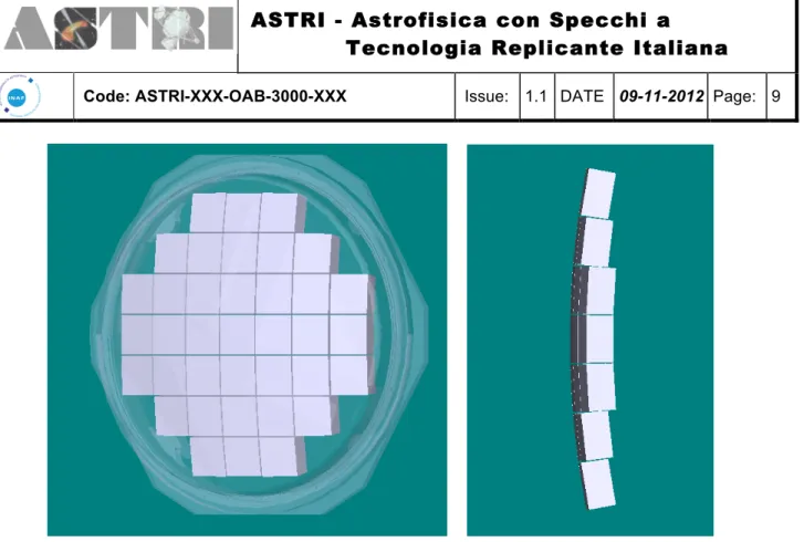
As example, placing a sort of truncated pyramid having the smaller base equal to the detection-‐active area of the UNIT in front of each of them, it is easy to recover the majority of the photons losses apart from the 12% that falls between the individual pixels. The top panel of Figure 7.1 shows the concept just described; while the bottom one present the comparison between two adjacent UNITS with and without the pyramid as simulated by ZEMAX. Finally, the Figure 7.2 shows the mechanical drawing. Moreover, using a proper glass type, i.e. with the index of refraction as high as possible and with good transmission in the desired energy band, it is possible to limit the thickness of those pyramids to few millimeters. The bottom side of these light concentrators can be treated with antireflection coating to minimize also the losses coming from the front reflection. An example of the coating is shown in Figure 7.3.
Figure 7.1 (top) Conceptual design of the reimaging system (drawing is not in scale). (bottom) Simulation of the refractive effect of the pyramids. The first quadrant top right has
no pyramid and looks dimmer than the other.
Figure 7.2 Mechanical drawing of the light cone concentrator. 1 1 2 2 3 3 4 4 5 5 6 6 A A B B C C D D g.l .3 A ng elo M an ga no 20 /0 6/ 20 11 Pr og et ta to d a C on tro lla to d a A pp ro va to d a D at a 1 / 1 Ed izio ne Fo glio D at a < Pe rc or so fil e> : 0,90 0,50 12,60 14,00 14 ,0 0 0,5 0 0,9 0 12 ,6 0 14 ,0 0 2,50 2,5 0 14,00 12,60
IA
SF
-IN
AF
Es pe rim en to : C TA -A ST R I 78,6 9 ° 70,20° 12 ,6 0 78 ,69° ° ,20 70
Figure 7.3 Transmission efficiency as function of the incident angle (20°, 30°, 40°, 50°, 60° and 70°) and wavelength
7.2
Reflective coatings
Coatings are very important for the optical systems. In this case, a fraction of the effective area as large as the 12-‐15% of that of the naked configuration can be gained simply using proper coatings. As an example, we report in Figure 7.4 four reflectivity curves related to the standard coating (Aluminum plus Quartz, Al+SiO2) and various multilayer coatings.
The red curve represents a pure dielectric coating; it is the ideal way to go, once its feasibility is proven. It gives the highest and uniform response and provides a way to select the wavelengths of interest; in particular, it suppresses the near infrared where the SiPM show also a good efficiency.
Figure 7.4 Comparison between possible coatings for enhancing the reflectivity of the M1 mirror.
7.3
Baffle
In the Schwarzschild-‐Couder layout the detector is facing the sky all the time. A proper baffle can be applied during the telescope observation mode in order to limit the amount of night sky background reaching the detector. For example, a cylinder properly sized (i.e. having the diameter of M2 and length as the distance M2-‐DET) can act as desired, see Figure 7.6.
Further studies of the telescope stray light can be found in [RD4]. Any reduction of the baffle height introduces photons contamination.
Figure 7.6 Drawing of the baffle concept. From left to right: the green hemisphere is M2 and the blue cylinder is the baffle. At the top of the grey tube is the focal plane with the detector
modules and the protective shutter windows opened (two lateral wings at the top of the tube).