
Household Wealth and Heterogeneous Impacts of a Market-Based Training Program: The Case of PROJOVEN in Peru
38
0
0
Full text
(2) Abstract This paper analyzes the relationship between households’ wealth and heterogeneous treatment impacts for a market-based training program that has benefited more than 40,000 disadvantaged individuals in Peru since 1996. We proxy long-run wealth by a linear index based on 21 household assets, and three main findings emerge. First, we find that voluntary choices among eligibles, rather than administrative choices, play a bigger role in explaining demographic disparities in program participation. Second, quantile treatment effects on the treated suggest important differences in program impacts at different quantiles of earnings, and strong differences in distributional impacts for men and women. Third, both parametricbased and semiparametric regression-matching estimates reveal that the poorest among the poor benefit the same from the program. It is the type of institution that provides the training services that largely accounts for the heterogeneity of the impacts. Key Words: training, program evaluation, factor analysis, poverty, quantiles, matching methods. JEL Classification Codes: I38, H43, C13, C14. 2. This work was carried out with financial and scientific support from the Poverty and Economic Policy (PEP) Research Network, which is financed by the Australian Agency for International Development (AusAID) and the Government of Canada through the International Development Research Centre (IDRC) and the Canadian International Development Agency (CIDA). We thank Guillermo Cruces, Ana Dammert, Habiba Djebbari, and Chris Ryan for useful comments and suggestions. We also thank seminar participants at the 2007 Poverty and Economic Policy Network Meeting in Lima. Veronica Montalva provided excellent research assistance..
(3) 1.. Introduction One of the most important empirical regularities that have emerged in the past 10. years in the field of microeconometrics is the pervasive evidence of heterogeneous responses to policy interventions (Heckman 2001). The existing literature on impact heterogeneity is based on social experiments carried out in developed countries. The work of Heckman, Smith, and Clements (1997), for instance, represents one of the first attempts to systematically analyze distributional impacts within the National Job Training Partnership Act Study (JTPA). Black, Smith, Berger, and Noel (2003) report impact heterogeneity on unemployment insurance recipiency within the Kentucky Profiling and Reemployment Services. Bitler, Gelbach, and Hoynes (2007, 2006) also find strong evidence against the common effect assumption using welfare experiments in the United States (Connecticut’s Jobs First Waiver Program) and Canada (Self-Sufficiency Project). For developing countries, there is scant evidence about impact heterogeneity in social programs. Djebbari and Smith (2005) and Dammert (2007) are, to the best of our knowledge, the first studies that explore heterogeneous impacts of conditional cash transfer programs in Latin America. Both studies find that program impacts on wealth and nutrition are greater for households who were at a higher level of wealth and nutrition prior to the program. Corresponding evidence for public-sponsored training programs is non-existent for developing countries. In this paper, we analyze whether the poorest among the poor benefit less from active labor market programs that target disadvantaged youth. This research question is particularly relevant in Peru, as well as in many developing countries, where one observes large income inequalities within poor households (e.g., Escobal, Saavedra, and Torero 1998) and where the training system excels in reproducing initial poverty conditions among youngsters (Valdivia 1997; Jaramillo, Díaz, and Ñopo 2007). We use a non-experimental training program, the Youth Training Program PROJOVEN, which has provided training to around 40,000 disadvantaged young individuals aged 16 to 24 since 1996. The PROJOVEN program corresponds to a new array of demanddriven training programs implemented in several Latin American countries in the midst of structural reforms in the mid-1990s. This “last generation” of active labor market policies is based on market-based approaches where public resources are assigned to training institutions via public bidding processes (see Chong and Galdo 2006). In this context, knowing whether this program produces the desired impacts or not constitutes a test of the effectiveness of market-based approaches in improving the employability and productivity of disadvantaged individuals.. 3.
(4) Partial institutional evaluations have found that the PROJOVEN program is an effective labor market initiative with mean treatment impacts ranging between 12 and 100 percent for earnings and between 0 and 15 percentage points for employment (Galdo 1998; Ñopo, Saavedra, and Robles 2001; and Chacaltana and Sulmont 2003). These “common effect” estimates are based on single-cohort data sets and focus on short-term treatment impacts. Two exceptions are Chong and Galdo (2006) and Díaz and Jaramillo (2006), which use data from five different cohorts to investigate the program’s short- and medium-term effects. The former investigates the relationship between the quality of the training services and beneficiaries’ subsequent earnings, while the latter focuses on mean treatment impacts. In this paper, we look at impacts across the entire distribution of the outcome variable. We use quantile treatment effects on the treated to estimate impacts on each percentile of the earnings distribution for men and women. Moreover, we exploit pre-treatment information on household assets to investigate the link between impact heterogeneity and households’ wealth status. This is important in assessing the program’s overall worth. For example, a program that raises the earnings of the most disadvantaged participants might be considered more successful than one that raises the earnings of only the least disadvantaged. Furthermore, we analyze the extent of ‘cream-skimming’ in PROJOVEN as the program has explicit performance rules that are tied to payments and penalties to training centers that may have an effect on the latter’s behavior regarding selection of trainees. We focus on both short- and medium-term treatment impacts using a comprehensive dataset that involves five different cohorts participating in the program from 1996 to 2004. To estimate heterogeneous treatment impacts across the wealth distribution, we construct an index based on the household asset information that PROJOVEN collects in order to assess eligibility of applicants. The basic methodology consists in approximating socioeconomic levels through a household’s asset index, which is based on principal component analysis of a determined number of asset variables. The method used here provides a simple technique for creating a long-run wealth proxy in the absence of either income or expenditure data (e.g., Filmer and Pritchett 2001; Gwatkin, Rutstein, Johnson, Pande, and Wagstaff 2000). We have three main findings. First, we find that voluntary choices among eligibles rather than administrative choices play a bigger role in explaining some demographic disparities in program participation when assessing the extent of cream-skimming in the PROJOVEN program. Second, the quantile treatment effects on the treated (QTT) show that impacts on earnings are concentrated among a relatively small number of participants and impacts for men are smaller but more evenly distributed than impacts for women. Third, both standard parametric and semiparametric matching models do not reject the null hypothesis. 4.
(5) that treatment does not vary with the individuals’ initial poverty level. It is the type of training institution, which is largely related to the quality of the training itself, that may explain the heterogeneity of the impacts of the program. The remainder of the paper is organized as follows. In section 2, we briefly discuss the institutional context of the PROJOVEN program. Section 3 provides an overview of the program design and operation. We then present the evaluation data in section 4. Section 5 presents the QTT impacts. In section 6, we develop the principal component analysis of household’s wealth status. In section 7, we report the parametric-based and semiparametric regression matching estimates. Finally, section 8 concludes. 2.. Institutional Analysis of PROJOVEN The economic context in which the PROJOVEN program was conceived was one of. vigorous economic recovery after the implementation of an aggressive stabilization and structural reform agenda. Indeed, Peru in the early nineties was one of the countries that moved faster in the direction of opening up the economy, eliminating price controls (literally overnight), and restricting the role of the State in the economy. At the same time, fiscal and monetary policy reforms were implemented in order to restore basic macroeconomic equilibrium and reduce inflation.1 After a period of adjustment-induced recession, by 1993 the economy was growing and in the following two years it was among the fastest growing economies in the region. Thanks to the brisk recovery and effective tax reform, by 1995 the country’s fiscal position had improved dramatically and increasing resources were being allocated to the social sector.2 The financial market and trade liberalization contributed to reduce the relative price of physical capital, and thus allowed firms to acquire new capital and hire high-skill workers. As a result, employment growth behaved procyclically, but it was not equitably distributed among different social or demographic groups. Specifically, both unemployment (14 percent) and underemployment (60 percent) rates for youth more than doubled those for adult workers.3 This one group seemed to be in need of extra help in order to take advantage of the new economic environment. Providing pertinent training to disadvantaged youth was the choice policy response in this context.. 1. See Jaramillo and Saavedra (2005) for a detailed account of policies during this period. Economic growth was a pre-condition for the Program to work. This was also one lesson from the Chilean experience (Marín 2003). 3 Total urban population of Peru is around 18 million people, of which 25 percent is between 16 and 24 years old. Participation in the labor force for this age group is large, accounting for more than onefourth. 2. 5.
(6) Furthermore, the high levels of expenditures and income inequality in Peru are well documented (e.g., Escobal et al. 1998).4 Because income heterogeneity may affect the distributional effects of the program, income distribution among PROJOVEN’s target population, roughly the two lowest income quintiles, constitutes relevant information for the present study. Table 1 reports income distribution indicators for youth and households of the two lowest income quintiles. We observe that the income gap between the lowest and second lowest per capita income quintiles is similar among households than among youth, and the gap is large. In fact, average labor income of youth belonging to the second lowest income quintile is more than two times the income of the most disadvantaged youth. In addition, significant inequality also appears within each income quintile. It is noteworthy that inequality is higher within the lowest income quintile, with a standard deviation representing around 40 percent of the mean, than inside the second lowest income quintile, in which the standard deviation represents around 20 percent of the mean. These facts already suggest potential impact heterogeneity in the PROJOVEN program along pre-treatment earnings. Income inequality typically goes together, to some extent, with education and labormarket inequalities; and all these three indicators can potentially influence the benefit level obtained by participants in the PROJOVEN program. In fact, even though general educational attainment is relatively high among urban youth, differences are significant across the distribution of income. Whereas the percentage of youth with complete secondary education is 72 percent in Metropolitan Lima and 60 percent in the urban area for youth belonging to the lowest income quintile, it reaches 90 percent in both areas for youth in the highest income quintile. Similarly, the percentage of youth with post secondary education is 31 percent in Metropolitan Lima and 25 percent in the urban area for the lowest income quintile while around 66 percent for both areas for the highest income quintile. Labor market outcomes of the targeted population are also a crucial aspect to consider for training programs. The unemployment rates for disadvantaged young individuals (21 percent) more than double that for non-poor youth (9 percent). Moreover, the activity rates are not only broadly unequal between them but the proportion of poor youth working in non-paid family jobs reaches almost 25 percent, far above the 12 percent observed for non-disadvantaged youth. Furthermore, labor-earnings gaps for the youth are not only consistently large across the age-earnings profile but also increase through the years. Whereas the average labor earnings for non-disadvantaged individuals aged 15 and 24 years old are approximately US$60 and US$150 respectively, the average labor earnings 4. The average monthly per capita expenditure is on average eight times higher for the highest income quintile than for the lowest income quintile in urban areas. On the income side, the difference is even bigger. The average monthly income is 14 times higher for the highest quintile than for the lowest one. Source: ENAHO 2004.. 6.
(7) for poor individuals are quite flat (US$45) throughout the whole youth age-earnings profile (15 to 24 years old). This important fact, also documented in Saavedra and Chacaltana (2001), supports the focus of active labor market policies on this disadvantaged group and, at the same time, favors the strategy for using control groups within the poor population in the evaluation of the PROJOVEN program. The identification of the treatment impacts is plausible because the outcomes for treated and untreated poor individuals will follow a parallel path in the absence of the program, provided a set of observable covariates. In sum, average educational attainment is relatively high for youth, but unequally distributed: poorer youth tend to have significantly lower educational levels. Naturally, earnings are low among poor youth. In addition, significant variance in earnings is found both between and within the two lowest quintiles of the income distribution. This means that not all participants are on equal footing to take advantage of PROJOVEN, suggesting a potential for heterogeneous impacts. 3.. The PROJOVEN Program. 3.1. Goals and Treatment The Youth Training Program PROJOVEN is an ongoing active labor market policy. that seeks to improve the productivity and employability of disadvantaged youth through labor training services. The PROJOVEN program was designed as a demand-driven program, with public and private training institutions competing for public resources through bidding processes. Since its creation in 1996, and for almost a decade, over 40,000 out-ofschool, unemployed poor individuals aged 16 to 24 years old have been selected as beneficiaries of PROJOVEN, and a total of 542 training institutions have participated in the program, providing more than 2,160 vocational courses. The PROJOVEN program provides funding for basic training in low-skill occupations. The treatment consists of a mix of in-class and on-the-job training organized into two sequential phases. The first consists of 300 hours of classes at the training center locations, roughly five hours per day for three months. The program covers the full cost of the courses. In addition, the program provides a stipend to trainees during these three months in the amount of US$2 dollars per day for men and women without children to cover for transportation and lunch, and of US$3 dollars for women with children under 6 years of age to cover childcare expenses. In the second phase, training institutions must place trainees into a paid, on-the-job training experience in private manufacturing firms for an additional period of three months. To ensure the paid on-the-job training experience, the program relies on a demanddriven mechanism that stipulates that all training centers must present, as part of their offers,. 7.
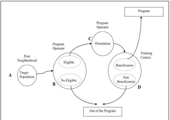
(8) formal agreements with private firms that guarantee internships remunerated (by the firm) at no less than the monthly minimum wage payment for each beneficiary. This design requires a strong match between the content of the training courses and the firm’s labor skill requirements. It supposes a strict coordination between the training institutions and firms when designing and implementing the training courses. As a result, the coverage of this program is limited because of its costly design (about US$515 dollars per trainee) and relatively intense package of services. 3.2. Eligibility, Participation, and Cream-Skimming Figure 1 shows the dynamic of the beneficiary selection process for any given cohort.. The program awareness strategy (position A) constitutes the first formal effort to reach out to the target population and aims to inform potential participants about the program’s benefits and rules. This first filter, under the responsibility of the program operator through local training offices, focuses only on those neighborhoods with a high concentration of households below the poverty line. Those prospective participants attracted by the expected benefits and perceived opportunity costs of participation voluntarily show up in the registration centers (position B), where qualified personnel determine their eligibility status. A standardized targeting system based on five key observable variables (poverty status, age, schooling, labor market status, and pre-treatment earnings) determines who is eligible and who is not. The low percentage of targeting errors shows the combination of self-targeting with individual assessment through objective indicators, which has been quite effective.5 According to the program’s operation rules, this process concludes when the total number of eligible individuals exceeds by around 90 percent the total number of slots available in each program. The eligibility status does not guarantee participation in the program. The program operator invites eligible individuals to an orientation process (position C), where they choose the courses they want to attend on a first-come-first-served basis. This process concludes when the number of eligible individuals exceeds by 75 percent the number of available slots in each course. Finally, the program operator sends this final pool of eligible applicants to the training institutions (position D). This is the only step in the process where training institutions intervene in the selection of participants and does not follow standardized criteria since each institution applies its own rules. Given a system of conditional payments based on center performance and flexibility to select from among the eligible population, training centers then have a strong incentive to. 5. Targeting errors have been documented to be below 10 percent (Arróspide and Egger 2000).. 8.
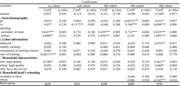
(9) enroll only those with the highest potential to complete and succeed in the courses.6 Thus, cream-skimming induced by performance standards is a legitimate concern in the PROJOVEN program because of its contribution to inequities in service delivery (Anderson, Burkhauser, and Raymond 1993). The availability of administrative data, where it is possible to identify eligibles from participants, provides an opportunity to disentangle cream-skimming from applicant’s selfselection decisions. From 1996 to 2004, the period for which we currently have data, there are 21,253 eligible individuals corresponding to the first, second, fourth, sixth, and eighth cohorts of the program in Metropolitan Lima. A simple comparison of observable characteristics between eligibles and participants shows that they differ in several dimensions associated with human capital and poverty variables. Eligibles are on average older and a greater percentage of them are men. Moreover, eligibles are on average less educated than participants. Furthermore, the analysis of dwelling characteristics suggests some differences in socio-economic status between eligibles and participants, particularly in the sixth and eighth cohorts. Finally, we observe for all cohorts that a higher percentage of eligibles were employed when registering for the program. Program rules suggest that the training centers may have the ability to select the less disadvantaged among the eligible population and thus, cream-skimming may arise from administrative choices. A closer look at the data reveals, however, that 47 percent of those youth eligible and registered to participate in PROJOVEN drop out before being sent to a training institution. This is a very large percentage considering the rather short period of time (two to three months) between registering as eligible and being assigned to a course. In practice, it means that training institutions do not have the ability to sort out eligible individuals given the rules concerning the number of slots available in the program. In fact, the de facto eligibles-participants ratio is less than 1.25/1.0. This evidence suggests that voluntary choices among eligibles rather than administrative choices play a bigger role in explaining some demographic disparities in program participation, and thus, it is insufficient to compare participant and eligible populations when assessing the extent of creamskimming, as Heckman, Heinrich, and Smith (2001) pointed out. We also look at the factors behind the decision to participate in the program. To identify which characteristics are associated with participation in the PROJOVEN program, a probit model was estimated for each cohort where the value 1 is assigned to beneficiaries and 0 to eligibles that do not pursue the application process to its conclusion (positions C. 6. Payments are structured in per capita terms according to the following scheme: 100, 80, 60, and 30 percent if completing both phases of the program, at least a month of on-the-job training, only in-class training, and at least a month of in-class training, respectively.. 9.
(10) and D in figure 1). Conceptually, one would expect that those dropping out are the ones facing the highest (direct and forgone) costs from participating. Opportunity costs will be higher for those who have relatively more human capital stock, those who already have a job, and those who would have to travel longer distances to reach the training institution. Participation and households’ wealth can also be positively correlated because of time preferences. Poorer households value more present income than future income. Table 2 reports the results. Gender is a significant predictor for three of five cohorts. Men are more prone to dropping out for all cohorts but the sixth. Results also indicate an inverse relation between age and participation, statistically significant for the sixth and eighth cohorts. It is the older who tend to drop out, which makes sense since they have a higher opportunity cost. Schooling is also a significant predictor across most cohorts. Eligibles with highest education level tend to participate in the program. This seems a counterintuitive result, as these youth have the highest opportunity cost. It is possible, however, that the time preferences effect dominates the opportunity costs effect within this economically disadvantaged population given the strong relationship between poverty and educational attainment. Thus, schooling may be proxy for socioeconomic status. The evidence regarding dwelling characteristics provides some backing for this interpretation as the estimates suggest that lower socio-economic status is associated with dropping out, although the evidence is not too conclusive as there are some mixed results across cohorts. The eighth cohort, the one with more observations and with more covariates available, reports most clearly the inverse relation between poverty and participation.7 4.. The Evaluation Data From 1996 to 2004, the PROJOVEN evaluation datasets consist of 10 different sub-. samples associated with five different cohorts of beneficiaries receiving treatment in Lima, and five corresponding comparison group samples.8 The beneficiary subsamples are selected by the program operator from a stratified random sample of the population of participants corresponding to the first, second, fourth, sixth, and eighth rounds of the program.9. 7. Benavides (2006) provides qualitative evidence from interviews with poor youth in the neighborhoods where the program operates that suggests that costs of participation are behind the decision to drop out. Unfortunately, we cannot identify in the data at hand dropouts from the eligible individuals that are not chosen for the training institutions. 8 These periods extend from November 1996 to April 1997; February 1998 to July 1998; March 1999 to August 1999; June 2000 to December 2000; and August 2001 to January 2002, respectively. 9 The total number of participants in these five cohorts is 1507, 1812, 2274, 2583, and 3114, respectively. The corresponding number of treated individuals in the random sample is 299, 321, 343, 405, and 421.. 10.
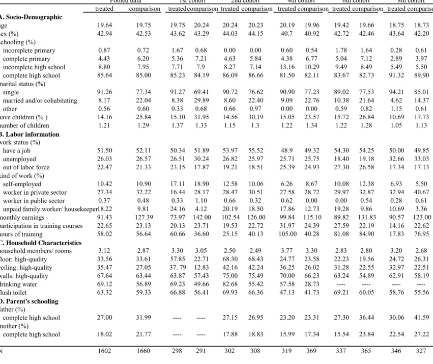
(11) Individuals in the corresponding comparison subsamples are selected from a random sample of “nearest-neighbor” households located in the same neighborhoods as those participants included in the evaluation sample aimed at reaching the same target population. In particular, once the treatment group individuals are chosen, a sample of comparison group individuals is selected by a survey fielded in the same poor neighborhoods where individuals from the treated group reside. The program operator uses the same eligibility instruments applied to the treatment sample and by pairing each beneficiary to a random neighbor who has the same sex, age, schooling, employment status, and initial poverty condition. The neighborhood dimension may have the ability to control some unobservables, including geographic segregation, transportation costs, and firms’ location, which may affect the propensity to work and the potential outcomes. This costly evaluation design greatly ameliorates support problems in the data, as we will see later. For each treated and untreated cohort combination, we have panel data collected in 4 rounds, including a baseline and 3 follow-up surveys taken 6, 12, and 18 months after the end of the program. The baseline survey provides rich information for all variables that define the eligibility status applied to treatment and comparison group individuals at the same calendar time. It also contains demographics, detailed labor-market information, dwelling characteristics, including source of drinking water, toilet facilities, and infrastructure (type of materials used in the floor, ceiling, and walls), which is used to build a wealth index. In fact, relevant factors affecting both the propensity to participate in the program and labor market outcomes are available. Moreover, the follow-up surveys provide detailed labormarket information for both treated and comparison groups, using the same definitions and variables as the baseline instruments. This minimizes potential biases due to misalignment in the measurement of variables, thus overcoming one of the main criticisms when solving the evaluation problem with non-experimental data (Smith and Todd 2005). The response rate to the initial survey was 100 percent and the attrition rates are small, ranging between 4 percent (12 months after the program) to 7 percent (18 months after the program).10 4.1. Comparison of Pre-Treatment Sample Means Table 3 compares the baseline means of several covariates for the treatment and. comparison samples for each one of five different cohorts. Column 2 shows the means using the pooled sample and columns 3 to 7 show the means for five different programs. In terms of demographic and socioeconomic characteristics, Panel A shows the effectiveness of the “neighborhood” strategy to balance the distribution of covariates that determine the eligibility status. Both groups have the same average age (19), sex ratio (42 percent are males), and. 10. For the eighth cohort we only have data available for the first two follow up surveys.. 11.
(12) schooling attainment (85 percent have completed high school). The p-values for all programs do not reject the null hypothesis of equality of means. However, the data show that both marital status and children variables have different distributions for treatment and control groups; estimated p-values reject the null hypothesis of equality of means in all cases. Panel B compares labor market characteristics for treatment and comparison samples. Both groups have the same proportion of individuals in and out of the labor force. Approximately 52, 25, and 22 percent of individuals were employed, unemployed, and out of the labor force, respectively. These non-significant differences are consistent across all cohorts. The type of work depicts a somewhat different pattern. A higher proportion of comparison individuals were working in the formal private sector (63 versus 54 percent) whereas a higher proportion of treated individuals were non-paid family workers (17 versus 10 percent). A comparison of monthly earnings also shows that treated units receive on average smaller earnings than their counterpart comparison sample, which is a steady result across all cohorts. Panel C compares households and dwelling characteristics. The analysis of dwelling characteristics shows that a higher proportion of treated individuals live in houses with somewhat better infrastructure and access to flush toilet and piped water. These differences, however, are not significant for several cohorts. Finally, the father’s schooling attainment is similar in both samples. In summary, table 3 shows that the treatment and comparison group individuals are similar in several dimensions, including sex, age, schooling, employment, father’s education, previous training, and family size. This result reveals the efficacy of the “nearest-neighbor” approach to construct the comparison sample because of the balance of all variables that define eligibility status between treated and untreated groups. On the other hand, the data also reveal some significant differences in three key variables: marital status, children, and unpaid family workers, which will be taken into account in the empirical strategy. 5.. Heterogeneous Treatment Impacts in PROJOVEN In this section we study whether there is heterogeneity in the distribution of earnings. impacts in the PROJOVEN program and discuss the hypothesis about distributional impacts in the program with estimates of quantiles treatment effects on the treated. 5.1. Quantile Treatment Effects on the Treated (QTT) Quantile regression has been used to address heterogeneous treatment impacts in. the context of training programs (Heckman et al. 1997, Friedlander and Robins 1997, Abadie, Angrist and Imbens 2002); welfare reform programs (Bitler et al. 2006, 2007);. 12.
(13) conditional cash transfer programs (Djebbari and Smith 2005, Dammert 2007); and profiling unemployment insurance programs (Black et al. 2003). The appeal of this approach lies in its flexibility to accommodate observed and unobserved heterogeneity (Djebbari and Smith 2005) and on the evidence that intra-group variation in quantile treatment effects greatly exceeds the inter-group variation in mean impacts (Bitler et al. 2006). This technique provides a convenient framework for examining how the impact varies at different quantiles of the untreated outcome distribution. Let Y1 and Y0 denote the outcome of interest in the treated and untreated states with corresponding CDFs. F1 ( y ) ≡ Pr[Y1 ≤ y ] and F0 ( y ) ≡ Pr[Y0 ≤ y ] . We can define the quantile treatment effect on the treated as Δ QTE|T =1 = y1|qT =1 − y0|qT =1 , where the qth quantiles of each distribution is defined by. y qj|T =1 = inf{ y : Fj ( y ) ≥ q | T = 1}, j = 0,1. This parameter of interest gives the difference in earnings between treatment group and comparison group members at any given percentile after conditioning on participation. Note that this parameter does not directly identify the distribution of impacts, which refers to the impact of the program on the earnings of an individual at that percentile unless the program satisfies very strong assumptions.11 To estimate the quantile treatment effect on the treated we use quantile regression of monthly earnings (Y) on an intercept and a discrete variable T = {0,1} . The impact estimate for a given quantile q distribution is the coefficient on the treatment indicator from the corresponding quantile regression.12 Without further assumptions, the quantile regression coefficients do not necessarily have a causal interpretation. As in the matching literature (e.g., Heckman et al. 1997), we then assume “selection on observables” to correct for selfselection into the program. We use the inverse propensity score-weighting approach (Imbens 2004). Denoting the estimated propensity score for person i as pˆ i ( x) , we define the inverse propensity score-weighting for treated and untreated units as:. wˆ1,i =. Ti. ∑ l =1Tl n. and wˆ 0,i =. pˆ i ( x) 1 − Ti , . 1 − pˆ i ( x) ∑ n Tl. (1). l =1. 11. If the ranking of individuals in the distribution of the outcome is preserved under the treatment, then this estimator is also informative about the distribution of impacts (Heckman et al. 1997). 12 For instance, estimating the quantile treatment effect at the 0.50 quantile involves taking the sample median for the treatment group and subtracting the sample median for the control group.. 13.
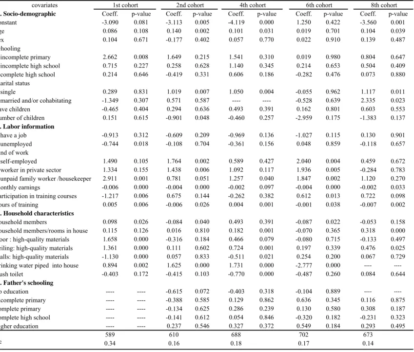
(14) which are used to estimate the effects of treatment on the treated.13 Under this approach, the empirical CDFs for Y1 and Y0 with normalized weights are given by:. (1/ n1 )∑ i =1 1 wˆ 1.i I (Y1 ≤ y ) n. Fˆ1 ( y ) =. ∑ i=1 wˆ1,i n1. (1/ n0 )∑ i =01 wˆ 0,i I (Y0 ≤ y ) n. and Fˆ0 ( y ) =. ∑ i =1 wˆ 0,i n0. (2). where n = n1 + n0 are the number of treated and comparison observations and I(.) is an indicator variable. This procedure corrects for bias in estimating quantiles of the counterfactual treated and control distributions when selection to treatment is based on observable variables and with the simple differences of sample adjusted quantiles then serving as consistent estimates of the population (see a formal proof in Firpo 2007). For the implementation of the weighting approach we estimate the propensity score that predicts the probability that the individual i is in the treatment group conditional on a rich set of baseline covariates, P (T = 1| X = x) . We estimate a logit model subject to the balancing test suggested by Dehejia and Wahba (1999).14 The set of conditioning covariates includes common demographic variables (sex, age, schooling, marital status, and number of children); labor market outcomes (past monthly earnings, employment status, type of work, previous training courses, duration of previous training); household characteristics (number of members, members/number of rooms, drinking water, flush toilet, dwelling’s quality materials); and father’s educational attainment. Table 4 reports the coefficients and standard errors for logit models estimated separately for each cohort. As expected, the covariates used to construct the comparison samples (age, sex, schooling, and employment status) are not significant predictors for program participation as they are balanced between treatment and comparison groups. In general, past earnings, experience, type of work, dwelling characteristics, father’s education, and family members/rooms are the most important predictors of participation in the PROJOVEN program. The estimates also show that married individuals and people with offspring are less likely to participate, although the coefficients are not significant for some cohorts.. 13. Alternatively, Bitler et al. (2004) estimate. wˆ i =. Ti 1 − Ti + pˆ i ( x) 1 − pˆ i ( x). to uncover treatment effects for the entire. population. 14 Parametric propensity score models that pass standard balancing tests are regarded as valid because they balance the distribution of pre-treatment covariates between matched units conditional on the propensity score. However, it is important to indicate that multiple versions of the balancing test exist in the literature, and little is known about their statistical properties or the relative efficiency among them.. 14.
(15) 5.2. QTT Estimates for Monthly Earnings We consider both earners and nonearners in our estimation to avoid neglecting the. substantial share of program impacts resulting from increased employment rather than higher earnings to treatment individuals who would have been employed anyway. In considering these estimates it is important to note the percentage of treatment and comparison group members that did not report earnings in follow-up dates. For men, 30 percent in the treatment group and 25 percent in the comparison group did not report earnings 6, 12, and 18 months after the program. For women, these numbers increase to 40 and 52 percent. These numbers imply two important points. First, impacts on labor earnings will be concentrated among a relatively small number of participants. Second, impacts on labor earnings will be larger and more unevenly distributed for women than for men. Figure 2 plots the quantiles treatment impacts for monthly earnings 6, 12, and 18 months after the program for both men and women pooled samples, to avoid large sampling variability due to small sample sizes. The associated dotted lines represent two-sided 90 percent bootstrapped confidence intervals. Figure 2 shows that women in the first 40th percentile of the earnings distribution report identically zero treatment effects, reflecting the large number of non-earners. Men, on the other hand, show zero or negative treatment impacts in the first 30th percentile. Furthermore, the uneven distribution of the nonzero estimates is an additional indication of the concentration of earnings impacts. Women between the 50th and 70th percentiles report the highest treatment impacts, whereas for the 80th and 90th percentiles the earnings gains decrease substantially in both the short- and medium-term. Men, on the other hand, show positive but small treatment impacts between the 40th and 70th percentiles, and negative treatment impacts for some percentiles in the bottom of the distribution. This last feature suggests that the strong push into employment for men relative to women indeed sacrificed some jobs at higher earnings levels. Strong disparities in labor participation rates between men and women in the Peruvian labor market are widely documented (Jaramillo, Díaz, and Ñopo 2007). Within the program sample, for example, the pre-treatment participation rate for men (62 percent) is much higher than that for women (45 percent). One would, therefore, expect that the primary effect of the PROJOVEN program should occur for those who find a job with program assistance but would not have found a job without the program. In addition, the PROJOVEN data show a large disparity in program completion rates between males and females. In fact, whereas 65 percent of women completed at least one month of on-the-job training, only 50 percent of men did the same. Thus, it is expected that treatment impacts are smaller for men yet, at the same time, more evenly distributed for them since the skills upgrading is less dramatic than that for women. Furthermore, in developing countries one observes that men. 15.
(16) and women face very different opportunity costs when deciding whether to participate in the labor market. Women are less forcefully pushed into employment because of household chores.15 As a result, women may be more selective about the jobs they take, allowing them to hold out for better job opportunities. This feature can strongly increase the unevenness of the impacts distribution for women relative to men because a larger percentage of women will decide to stay out of the labor force. Regardless of the certainty with which these underlying patterns may be inferred, figure 2 clearly shows higher treatment impacts for women across most percentiles of the earnings distribution and, at the same time, higher heterogeneity of the impacts on the distribution of earnings. For instance, whereas the impact on the median of the earnings distribution is US$22 for men 6 months after the program, it almost doubles for women (US$41). Moreover, the range of QTT earnings impacts is [US$0, US$24] for men and [US$0, US$71] for women 6 months after the program. These strong differences are the same whether we measure the impacts 6 or 18 months after the program.16 We asked if it is possible to link the strong evidence on QTT impact heterogeneity to differences in household wealth. Put differently, are the poorest among the poor the ones located at the bottom percentiles of the QTT earnings distribution? These questions cannot be answered in the context of our QTE estimation unless we observe individual impact estimates for all sample members. If so, we can examine the frequency of the QTT estimates across different wealth categories. Rather, we test the role of households’ wealth as a source of heterogeneous treatment impacts by implementing alternative econometric estimators (such as standard OLS and matching methods) which allow us to test differential mean treatment effects across different wealth categories. It is noteworthy that this strategy represents a lower bound to the true extent of impact heterogeneity since the intra-group variation embodied in quantile treatment effects greatly exceeds the inter-group variation in mean impacts. 6.. Measuring Household’s Wealth Because household income or expenditure data are not readily available for. treatment and comparison group individuals, we construct an asset index based on household asset information that PROJOVEN collects to assess eligibility of applicants following factor analytic methods. In contrast to expenditure data that is highly variable and sensitive to transitory fluctuations (Jalan and Ravallion 1998), the asset index is more stable. 15. Research shows significant gender differences in time use in developing countries, with young men more likely to work for pay and young women more likely to do domestic chores. See, for instance, Levison and Moe’s (1998) findings for Peru. 16 All figures in real values of December 2001. The exchange rate (dollar/sol) was 3.4.. 16.
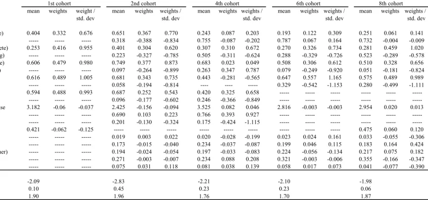
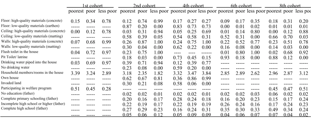
(17) (Fields 1998, Skoufias 1999) and contains less measurement error (Filmer and Pritchett 2001) when predicting a household’s wealth status. By aggregating household assets, the index represents a proxy for long-run economic status rather than a measure either of current welfare or poverty. In fact, we are only establishing a relative measure -households’ ranking within the distribution-, which makes sense in the context of our empirical problem because all treated and comparison individuals are by definition below the poverty line. Because the weight each asset receives is not grounded theoretically, it is recommendable to perform empirical validation exercises to establish the robustness of the index. Evidence for some developing countries suggests that this approach is a robust measure of household wealth (Filmer and Pritchett 2001) and comparable to the results emerging from consumption expenditures in a sample of 19 countries (Wagstaff and Watanabe 2003). 6.1. Constructing the Wealth Index The baseline surveys the first, second, fourth, sixth, and eighth rounds of the. PROJOVEN program, and includes information on 21 poverty indicators that can be grouped into four types: characteristics of the household’s dwelling (six indicators for the building materials used, two indicators for toilet facilities, two indicators for the source of drinking water, two indicators about rooms in the dwelling); household landownership, with two indicators; household’s participation in welfare programs; and parent’s education attainment. Escobal et al. (1998) show that these assets play a pivotal role in explaining the poverty status of Peruvian households in the 1990’s using expenditure data. To aggregate these various asset indicators into one variable to proxy for household wealth, we use the statistical procedure of principal components. The mathematical steps to perform the principal component analysis are detailed in Smith (2002). This technique essentially consolidates the data around the covariance structure of the variables under the assumption. In this particular context, this means that household’s long-run wealth explains the maximum variance-covariance in the wealth variables. Intuitively, it extracts from a set of variables those few orthogonal linear combinations of all the variables that capture the largest amount of information that is common to all of the variables (maximum variance). Then, it finds the second linear combination for the variables, orthogonal to the first, with maximum remaining variance, and so on. The first linear combination is called the first principal component of the set of variables. Once the asset index is obtained for each individual in the dataset, the individuals are ranked by their asset index score and divided into quintiles. Table 5 reports the weights (or scoring factors) from the principal component analysis implemented separately for each. 17.
(18) cohort. The mean of the index is 0 for all rounds with standard deviation in the range 1.46 to 1.93. Because the index ranks households within each distribution, the weights differ from program to program, although we observe similar patterns (signs) for all variables. In general, the characteristics of the household’s dwelling receive the highest weights across all programs. Because all the variables (except members/rooms) are categorical ones, it is easy to interpret the weights: a move from 0 to 1 changes the index by a factor equal to weight/standard deviation (reported in columns 3, 6, 9, 12, and 15). For instance, Column 3 shows that a treated or comparison individual that lives in a household with flush toilet has a wealth index higher by 1.005 than one who does not. The last three rows of table 5 report the mean wealth index for three different groups of individuals that are assigned to the bottom quartile (“poorest”), second and third quartile (“poor”), and upper quartile (“less poor”), according to the value of their index. The difference in the mean index between the “poorest” and “less poor” individuals, as well as between the “less poor” and “poor”, is remarkable. To evaluate the internal validity of the wealth index we investigate the mean distribution of the asset variables across the different percentiles of the PROJOVEN population. We expect that the “poorest” group individuals have the lowest level of asset ownership whereas the “less poor” group individuals represent the highest level. Table 6 reports the average asset ownership across the bottom (25 percent), middle (50 percent), and upper (75 percent) quartiles for all programs. We find, as expected, that the asset ownership differs consistently across these groups of individuals in all rounds of the program. By looking at the first three columns, we observe for instance that, whereas only the 3.3 percent of the “poorest” individuals have access to potable water, this percentage increases to 68 percent for “poor” individuals and to 97 percent for “less poor” individuals. Likewise, the house ownership increases from 36 percent (“poorest”) to 85 percent (“poor”) and 99 percent (“less poor”) in the second round of the program. Also, 62 percent of the “poorest” individuals in the fourth round of the program live in houses with low-quality walls (matting) versus 22 percent for the “poor” individuals and 0 percent for the “less poor” individuals. To evaluate the external validity of our wealth measures we use a standard representative household survey, the Encuesta Nacional de Hogares (ENAHO), conducted in 2000 by Peru’s national statistical agency, the Instituto Nacional de Estadística e Informática. The availability of consumption expenditures and income data allows us to compare an asset index with both household per capita consumption expenditures and. 18.
(19) household per capita income. The asset index is based on the same variables used in the PROJOVEN program with all measures computed only for Metropolitan Lima.17 The results show a considerable fit between the wealth index and expenditures and income measures. The Spearman rank correlations across households are slightly higher when using the expenditures measures (0.59, p=0.000) rather than the income measures (0.54, p=0.000). We further examine the degree of agreement among the different measures by comparing how well the three classification measures overlap. We assigned households to the poorest 40, middle 40, and richest 20 percentiles using all three measures of wealth. Table 7 reports the results, where three main findings emerge. First, by looking at the expenditures measure (upper panel) we observe that 70 percent of those classified into the poorest category by consumption expenditures are also classified as poorest by the asset index. Moreover, only 4 percent of those classified into the poorest category by expenditures appear in the richest category by the asset index. Second, the classification on the middle and rich categories show somewhat less agreement, with 55 and 54 percent of those classified into these categories by consumption expenditures are also classified as middle and rich for the asset index. Importantly, only 3 percent of those classified into the richest category by expenditures appear in the poorest category by the asset index. Third, the results for the income measure (lower panel) are quite similar to those obtained with the expenditures data, which reassures us on the consistency among the three measures. 7.. Treatment Impacts across Wealth Status. 7.1. Parametric Treatment Impacts In this section we explore the heterogeneity of the impacts as a function of the. estimated wealth index. It considers variation in treatment impacts through the interaction of the treatment indicator with the estimated long-run wealth status. If the PROJOVEN targeting mechanism is effective, one expects the poorest individuals to benefit the most from the program. Let. Y1 (q). be the potential outcome in the treatment state (T = 1) for an individual. who is in the wealth quantile q and let. Y0 (q ). be the potential outcome in the untreated. state (T = 0) . Our parameter of interest is the impact of treatment on the treated, which estimates the mean effect of attending a training course rather than not participating on the individuals who attend the course: 17. The survey has 2,572 respondent households. Household consumption and household income are computed by the statistical agency based on the survey’s more than 40 pages of questions on expenditures, consumption, and income. The data are available at www.inei.gob.pe/English/Consulta_por_Encuesta.asp.. 19.
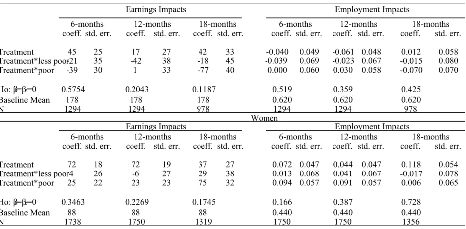
(20) ΔTT = E (Y1 (q) − Y0 (q) | T = 1) = E (Y1 (q ) | T = 1) − E (Y0 (q) | T = 1). (3). While E (Y1 (q ) | T = 1) may be estimated from the observed treatment sample, the right-hand side of the equation (3) contains the missing data E (Y0 (q ) | T = 1) . Because program participation in PROJOVEN depends on both observed and unobserved characteristics which lead to self-selection, one can proceed under the assumption that the distribution of systematic and unobserved differences varies across T=1 and T=0 but not over time within groups, which is the standard assumption of difference-in-differences models. However, this approach may be sensitive to the specific definition of the ‘before” period if we observe a drop in the mean earnings of participants prior to program entry (Ashenfelter 1978). In fact, Chong and Galdo (2006) document the existence of Ashenfelter’s Dip in the PROJOVEN program, which may lend an upward bias to the standard parametric difference-in-differences estimates. We then use an alternative econometric estimator that is consistent when the model of program participation stipulates pre-program earnings dip. We use a regression-based estimator of the difference between the post-treatment earnings of treatment and comparison group members, holding constant the level of pre-treatment earnings and a set of control variables (LaLonde 1986). We compare treatment and comparison individuals through a linear regression of the outcome variables Y (i.e., monthly earnings and employment) on the treatment status (T) and interactions between T and dummy variables indicating whether the individual i is in the top (“less poor”), middle (“poor”), or bottom (“poorest”) percentile of the wealth index distribution,. Yit = δ 0 + δ1q3i + δ 2 q2i + β 0Ti + β1Ti * q3i + β 2Ti * q2i + γ Yi ,t −1 + X it 'α + ε it .. (4). The individuals in the “poorest” group (q1) are the omitted group and, therefore, the implicit counterfactual. The interaction terms are expected to be positive if individuals from “less poor” (q3) and “poor” households (q2) benefit more from the program than individuals living in the “poorest” households (q1). Equation (4) also controls for other baseline household and individual characteristics (X) to account for empirical differences in the covariate distribution between treatment and comparison groups. The X-vector includes sex, age, schooling, marital status, offspring, and pre-treatment participation in training courses. This parametric approach estimates the effect of a treatment under the assumptions of selection on observables, and that simple linear conditioning on the covariates suffices to eliminate selection bias. We test whether the program impact along the wealth index is the same for all individuals by testing the following hypothesis:. 20.
(21) Ho : β1 = β 2 = 0. Rejecting this null hypothesis is evidence of heterogeneous program impacts emerging from differences in individuals’ wealth status. Table 8 reports the results for both monthly earnings and employment outcomes for men (Panel A) and women (Panel B) samples. Two main results emerge. First, we do not reject the null hypothesis that treatment does not vary with the individuals’ initial poverty level. The p-values are above 0.10, and this is a stable result for both men and women and independent of whether we measure the impacts 6, 12 or 18 months after the program and the outcome of interest. This result suggests that the strong treatment heterogeneity on the earnings distribution emerging from the QTT approach is not due to the variation in the initial poverty level of the beneficiaries. Second, both earnings and employment treatment estimates are larger for women rather than men. This finding is in line with our QTT estimates. 7.2. Matching Treatment Impacts We relax any linear assumption that may mask the earnings-wealth relationship by. taking weighted averages over the outcomes of observationally similar untreated individuals. We implement both difference-in-difference and cross-section propensity scores matching methods that are better equipped to deal with the pre-treatment earnings dip after forcing one to compare individuals with the same pre-treatment observable characteristics. The identifying assumption justifying this matching estimator is that there is a set of conditioning variables X such that:. E (Y0t (q) − Y0t ' (q ) | X , T = 1) = E (Y0t (q ) − Y0t ' (q) | X , T = 0). (5). where t’ and t refer to before and after the start of the program (Heckman et al. 1997). This conditional independence assumption ensures that after conditioning on a rich set of observable variables, the outcomes for treated and untreated individuals follow a parallel path. Matching methods force us to compare comparable individuals by relying on the common support assumption:. Pr(T = 1| X ) < 1 for all X.. (6). The support condition ensures that for each X satisfying assumption (5) there is a positive probability of finding a match for each treatment individual. In this sense, matching forces us to compare comparable individuals in a way that standard regression methods do not. Less than five percent of the observations are out of the empirical overlapping region,. 21.
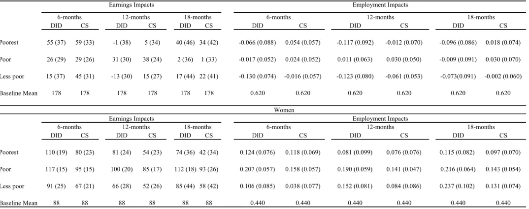
(22) which illustrates the relative efficiency of constructing comparison groups among eligible “neighbors”.18 We use local linear kernel matching that relies on standard kernel weighting functions that assign greater weight to individuals who are similar in terms of the estimated propensity score (Heckman et al. 1998). The price to be paid for the greater flexibility of local linear matching is the selection of the bandwidth parameter that achieves the best possible tradeoff between bias and variance (Imbens 2004). We choose the bandwidth h to minimize the approximation to the mean integrated squared error (MISE) of the estimated counterfactual mean regression function associated with a particular bandwidth given by:. ⎛ 1 n0 2⎞ MISE(h) = arg min ⎜ ∑ ( (Y0 jt − Y0 jt ' ) − mˆ − j ( pˆ ( x j ), h) ) ⎟ . h ⎝ n0 j =1 ⎠. (7). ˆ − j ( pˆ ( x j ), h) denotes the estimated conditional mean function for the where m untreated outcome evaluated at pˆ ( x j ) using all of the untreated units except unit “j”. The benefit of this cross-validation approach comes from using out-of-sample forecasts rather than in-sample fit to guide the bandwidth choice. This approach implicitly weights the MISE calculation by the distribution of estimated propensity scores in the untreated sample. Operationally, this approach proceeds via a grid search over a set of candidate bandwidths specified in advance.19 Table 9 presents both difference-in-difference (DID) and cross-section (CS) matching estimates for monthly earnings and employment outcomes for men (panel A) and women (panel B). Within each panel, we report three different parameters of interest: the average treatment effect on those located on the top quantile of the wealth index (“less poor”), the average treatment effect on those located in the second and third quantile (“poor”), and the average treatment effect on those located in the bottom quantile (“poorest”). In all cases, we estimate the counterfactuals using the full set of comparison group observations. The point estimates for the treatment impacts are presented along with their corresponding bootstrapped standard errors estimated with 500 replications. The results show three main patterns. First, there is again no evidence that the poorest among the poor benefit less from the PROJOVEN program. In this aspect, the PROJOVEN program is very effective in not reproducing commonly observed wealth gaps. 18. To impose the support condition we follow the “trimming” procedure proposed by Heckman et al. (1998). The grid for the bandwidth search equals [0.05, 0.10,…, 2]. Relative to their frequency in a random population, the treatment group individuals are oversampled. Thus, we apply the matching methods to choice-based sampled data, and we thus use the log of the odd ratio pˆ ( x) /1 − pˆ ( x) as the matching variable (Heckman and Todd 1995). 19. 22.
(23) on labor outcomes in the Peruvian labor market. On the contrary, the matching estimates for women suggest that the “less poor” individuals are benefiting somewhat less than the “poor” individuals. Second, the matching estimates show the PROJOVEN program is an effective, active labor-market initiative for women. For instance, 6 months after the program the earnings treatment impacts on the treated ranges from US$20 to US$27 and from US$23 to US$32 for women located on the top and bottom quantiles of the wealth index. Employment effects are also positive for women but not for men, reinforcing the previous OLS estimates. Third, the cross-section matching estimates are lower than the difference-in-difference estimates. This is explained by the existence of Ashenfelter’s dip in the PROJOVEN data. Notice, however, that these differences are modest. Because not everyone receives training in the same institution and the same occupation, both the type of training center and the occupation in which the participants receive training may potentially account for the heterogeneity of the treatment impacts. For instance, the quality of the training services may differ greatly among institutions as long as the level of educational specialization and experience varies, leading to potential heterogeneity of the impacts. Likewise, some occupations may have higher returns in the labor market independent of the quality of the training itself. There are five types of training providers in the PROJOVEN program: private business/manufacturing. firms,. non-governmental. organizations. (NGOs),. post-school. technological institutes (ISTs), occupational training centers (CEOs), and sectoral training centers.20 Using the quality index constructed by Chong and Galdo (2006) we find strong variation in the quality of the training services among these institutions. On average, private manufacturing firms offer the lowest quality (0.38), while sectoral training centers offer the highest one (0.68). With regard to the type of occupation, the distribution of funded courses in the PROJOVEN program is highly concentrated in textiles and apparel (45 percent) followed by services (22 percent), mechanics and metalworking (16 percent), and construction, carpentry, and shoemaking (15 percent). To address the role of training centers and occupation as possible sources of the heterogeneity in the impact of the program, we estimate a linear regression model using data on program participants who have enrolled in different training institutions and. 20. The sectoral training centers in Industry (SENATI), Construction (SENCICO), Telecommunications (INICTEL), and Tourism (CENFOTUR) are funded by legally mandated contributions from employers in their respective sectors and primarily provide training specific to each one’s own sector, both in the form of careers or specific courses. The post-school technical institutes (ISTs) can be either public or private. Like the sectoral training centers, they are open to secondary school graduates and offer both three to four-year technical careers and individual courses. Finally, outside of the academic hierarchy, and unconnected to it, are the occupational training centers (CEOs). Admission to a CEO is not conditioned to any basic schooling requirement.. 23.
(24) courses.21 We include a set of dummy variables that reflects the type of training center and occupation. The omitted categories are private business/manufacturing firms and mechanics/metalworking, respectively. We also include controls for other baseline household and individual characteristics, including the wealth index, to account for empirical differences in the covariate distribution among the treated individuals. Table 10 reports the results for both monthly earnings and employment outcomes. Three main patterns emerge. First, there is strong heterogeneity in the returns to training depending on the type of institution where one receives training. On average, individuals attending a sectoral training institution show the highest returns while individuals attending private business/manufacturing firms show the lowest ones. This is a robust result for both men and women and independent of the outcome of interest. Second, the level of heterogeneity is larger for women rather than men, which is consistent with the QTT results. Third, the type of occupation does not matter. A test of the joint significance for the occupation dummy variables is rejected for both outcomes of interest. Overall, these results reveal that neither the wealth status nor the occupation is the source of heterogeneity in the PROJOVEN program. It is the type of training institution, which is largely related to the quality of the training itself, that may explain the heterogeneity of the impacts of the program. 8.. Conclusions and Policy Discussion The Youth Training Program PROJOVEN corresponds to a new array of demand-. driven training programs implemented in Latin America in the 1990s in the midst of structural reforms in the labor markets. Similar programs have been implemented in Argentina, Chile, Uruguay, and Colombia. This “last generation” of active labor market policies is based on market-based approaches where public resources are assigned to training institutions via public bidding processes. In this context, knowing whether this program produces the desired impacts or not constitutes a test of the effectiveness of market-based approaches to improve the employability and productivity of disadvantaged individuals. Several of the findings presented in this report are of interest to policy makers. First, policy makers interested in enhancing equity aspects of social programs should be interested in the process of participation. We find that voluntary choices among eligibles and not administrative choices play a bigger role in explaining some demographic disparities in program participation. Identification of the factors that prevent the most disadvantaged from participating would be an important step in order to establish better targeting strategies.. 21. We also estimate the same linear regression model, including the comparison sample and a dummy variable for treatment status. None of the qualitative results changed.. 24.
(25) Second, regarding the impact of the program, the results indicate that PROJOVEN’s design is not only an effective mechanism to enhance productivity of economically disadvantaged youth, but it is also equity enhancing among groups of varying poverty levels. This result is likely related to the demand-driven mechanism, which ensures training only on those occupations with assured labor demand that avoids reproducing initial poverty conditions among youngsters.22 Third, the positive assessment of the PROJOVEN program should be tempered by the existence of a high concentration of positive earnings impacts around the 40th and 70th percentiles. In particular, the strong heterogeneity of the treatment impacts can be explained by the type of institution that provides the training services rather than by the wealth status or the occupation in which the participants receive training. In this respect, the heterogeneity in the quality of the training services seems to be the determinant for the size of the treatment impacts as suggested by Chong and Galdo (2006). More research in this direction would be welcome. For instance, it seems more important for the program to rely more on the training services of sectoral training centers rather than private business firms. Fourth, both earnings and employment impacts are larger for women rather than for men, which suggest that interventions such as PROJOVEN are relevant options for policy makers interested in reducing labor market gender gaps. This is possibly associated with the fact that because of opportunity costs (compounded with discrimination, among other factors) women face greater difficulties in getting access to proper employment. Within this context, exposing the participant to a package of basic training and practical experience in the firm seems to go a long way towards changing the labor market prospects of the young women participating in the program. It should be noted that PROJOVEN’s design includes a stipend for single mothers to cover costs of childcare. This information is also important for the discussion of which groups should be targeted by this type of policy in the context of tight public budgets. Five, PROJOVEN seems to be a better fit to improve earnings of participants than changing their employment status, as impacts on earnings are consistently higher than on employment. In other words, while the training intervention seems adequate to produce changes in earnings it does not seem to work the same for employment. Thus, if the goal of the government is to improve employment opportunities of those youth who do not have a job, policy makers should consider specific modifications to the program. Short of starting a different program, it may be a good idea to experiment with a training module within the PROJOVEN setting specifically oriented to this goal.. 22. The Peruvian training system excels in reproducing initial poverty conditions because poorer individuals only have access to very low-quality training institutions, perpetuating large labor earning gaps (Valdivia 1997).. 25.
(26) References Anderson, K., R. Burkhauser, and J. Raymond. 1993. “The Effect of Creaming on Placement Rates under the Job Training Partnership Act.” Industrial and Labor Relations Review. 46 (4): 613-624 Arróspide, M. and P. Egger. 2000 “Capacitación Laboral y Empleo de Jóvenes en el Perú: La Experiencia del Programa PROJoven.” OIT. Ashenfelter, O. 1978. “Estimating the Effect of Training on Earnings.” Review of Economics and Statistics 60: 47-57. Benavides, M. 2006. Para Acercarse a los que se Alejan. Exclusión, Jóvenes y Políticas Públicas. Final Report for Research Department, Inter American Development Bank. Black, D., J. Smith, M. Berger, B. Noel (2003): “Is the Threat of Reemployment Services More Effective than the Services Themselves? Experimental Evidence from the UI System”, American Economic Review, 93 (4) : 1313-1327. Bitler, Marianne, Jonah Gelbach, and Hilary W. Hoynes. 2007. “Distributional Impacts of the Self-Sufficiency Project.” Journal of Public Economics, Forthcoming. Bitler, Marianne, Jonah Gelbach, and Hilary W. Hoynes. 2006. “What Mean Impact Miss: Distributional Effects of Welfare Reform Experiments.” American Economic Review, 96 (4). Chong A., and J. Galdo J. 2006. “Does the Quality of Public-Sponsored Training Programs Matter? Evidence from Bidding Processes Data.” Manuscript. Chacaltana, J. and D. Sulmont. 2003. “Políticas Activas en el Mercado Laboral Peruano: El Potencial de la Capacitación y los Servicios de Empleo.” Lima, Peru: Consorcio de Investigaciones Económicas y Sociales (CIES). Dammert, A. 2007. “Heterogeneous Impacts of Conditional Cash Transfers: Evidence from Nicaragua”, Manuscript. Dehejia R. and S. Wahba. 1999. “Causal effects in Non-Experimental Studies: Re-evaluating the Evaluation of Training Programs.” Journal of the American Statistical Association 94: 1053-1062. Díaz, J. and M. Jaramillo. 2006. “An Evaluation of the Peruvian Youth Labor Training Program – PROJOVEN”. Washington, D.C.: Office of Evaluation and Oversight, Inter American Development Bank, working paper WP-10/6. Djebbari H., and J. Smith. 2005. “Heterogeneous Program Impacts in PROGRESA”, Manuscript. Escobal J., J. Saavedra, and M. Torero. 1998. “Los Activos de los Pobres en el Peru” GRADE, Lima. Fields G. 1998. “Income Mobility: Meaning, Measurement, and Some Evidence for the Developing World.” Manuscript. Filmer, D. and L Pritchett. 2001. "Estimating Wealth Effects without Expenditure Data--Or Tears: An Application to Educational Enrollments in States of India" Demography , Volume 38, Number 1, pp. 115-132 Firpo, S. 2007. “Efficient Semiparametric Estimation of Quantile Treatment Effects.” Econometrica, 75(1):259-276. Friedlander, D. and P. Robins. 1997. “The Distributional impacts of Social Programs.” Evaluation Review, 21(5), pp. 531-553.. 26.
(27) Galdo, J. 1998. “Evaluación de Proyectos de Inversión Social: Impacto del Programa de Capacitación Laboral Juvenil PROJOVEN.” Boletín de Economía Laboral 9, Ministerio de Trabajo y Promoción Social. Gwatkin, D., R. Rutstein, K. Johnson, R. Pande and A.Wagstaff. 2000. Socio-Economic Differences in Health, Nutrition and Population in [44 countries]. Washington, D.C.: The World Bank, Health, Nutrition and Population Department. Heckman, J. 2001. “Micro data, Heterogeneity, and the Evaluation of Public Policy: Nobel Lecture.” Journal of Political Economy 109: 673-748. Heckman, J., H.R. LaLonde, and J. Smith. 1999. “The Economics and Econometrics of Active Labor Programs.” In: O. Ashenfelter and D. Card, eds. Handbook of Labor Economics, Volume 3A. Amsterdam: North Holland, pp. 1865-2097. Heckman, J. and J. Smith, 1999. “The Pre-Programme Earnings Dip and the Determinants of Participation in a Social Programme. Implications for Simple Programme Evaluation Strategies.” Economic Journal 109(457): 313-348. Heckman, J., H. Ichimura, J. Smith, and P. Todd. 1998. “Characterizing Selection Bias Using Experimental Data.” Econometrica 66(5): 1017-1098. Heckman, J., H. Ichimura, and P. Todd. 1997. “Matching as an Econometric Evaluation Estimator: Evidence from Evaluating a Job Training Programme.” Review of Economics Studies 64(4): 605-654. Heckman, J., J. Smith, and N. Clement. 1997. “Making the Most Out of Program Evaluations and Social Experiments: Accounting for Heterogeneity in Program Impacts.” Review of Economic Studies 64: 421-471. Heckman, James, Carolyn Heinrich and Jeffrey Smith. 2001. “The Performance of Performance Standards.” Journal of Human Resources. 37(4). 778-811. Imbens, G. 2004. “Nonparametric Estimation of Average Treatment Effects under Exogeneity.” The Review of Economics and Statistics, 86: 4-29 Jalan, J. and M. Ravallion. 1998. “Transient Poverty in Postreform Rural china.” Journal of Comparative Economics, 26:338-357 Jaramillo, M, and J. Saavedra. 2005. "Governability, Reforms and Economic Performance in 1990s Peru.” In: A. Solimano (ed.), Political Crises, Social Conflict and Economic Development: The Political Economy of the Andean Region. Nueva York: Edward Elgar Publishing. Jaramillo, M., J. Díaz and H. Ñopo. 2007. “La Investigación Sobre el Mercado Laboral Peruano: Instituciones, Capacitación y Grupos Desfavorecidos”. GRADE, Investigación, Políticas y Desarrollo en el Perú. Lima: GRADE. LaLonde, R. 1986. “Evaluating the Econometric Evaluation of Training Programs with Experimental Data”, The American Economics Review, 76(4), 604-620 Levison D. and K. Moe. 1998. “Household work as a deterrent to schooling: An analysis of adolescents girls in Peru.” Journal of Developing Areas. 32(3): 339-356. Marin J. 2003. “Chile Joven: Trayectoria y Resultados del Programa de Capacitación Laboral de Jovenes.”, OIT. Ñopo, H., J. Saavedra, and M. Robles. 2001. “Una Medición del Impacto del Programa de Capacitación Laboral Juvenil PROJOVEN.” GRADE, Lima, Peru. Saavedra, J. and J. Chacaltana. 2001. “Exclusión y Oportunidad: Jóvenes Urbanos y su Inserción en el Mercado de Trabajo y en el Mercado de Capacitación”, GRADE.. 27.
(28) Skoufias, E. 1999. “Krismon and Its Impact on Household Welfare: Preliminary Evidence form Household Panel Data from the 100 Village Survey in Indonesia.” Manuscript. Smith, L. (2002) “A Tutorial on Principal Component Analysis.” Manuscript. Smith, J. and P. Todd. 2005. “Does Matching Overcome LaLonde’s Critique of NonExperimental Estimators? Journal of Econometrics 125(1-2): 305-353. Stecklov, G., A. Bommier, and T. Boerma. 1999. “Trends in Equity in Child Survival in Developing Countries: A Illustrative Example using Ugandan Data.” Manuscript. Valdivia, N. 1997. “ La Relacion entre Educacion Superior, Empleo y Movilidad Social: el Caso de los Tecnicos Profesionales en Lima Metropolitana”. GRADE, Peru. Wagstaff, A. and N. Watanabe. 2003. “What Difference does the Choice of SES Make in Health Inequality Measurement?” Health Economics. 28.
Figure

+6
Related documents