H. Roussel
Institut d’Astrophysique de Paris, Universit´e Pierre et Marie Curie (UPMC), CNRS (UMR 7095), 75014 Paris, France
ABSTRACT
Scanamorphos is one of the public softwares available to post-process scan observations performed with the Herschel photometer arrays. This post-processing mainly consists in sub-tracting the total low-frequency noise (both its thermal and non-thermal components), masking high-frequency artefacts such as cosmic ray hits, and projecting the data onto a map. Although it was developed for Herschel, it is also applicable with minimal adjustment to scan observations made with some other imaging arrays subjected to low-frequency noise, provided they entail sufficient redundancy; it was successfully applied to P-Art´emis, an instrument operating on the APEX telescope. Contrary to matrix-inversion softwares and high-pass filters,Scanamorphos
does not assume any particular noise model, and does not apply any Fourier-space filtering to the data, but is an empirical tool using purely the redundancy built in the observations – tak-ing advantage of the fact that each portion of the sky is sampled at multiple times by multiple bolometers. It is an interactive software in the sense that the user is allowed to optionally visu-alize and control results at each intermediate step, but the processing is fully automated. This paper describes the principles and algorithm ofScanamorphosand presents several examples of application.
Subject headings:Astronomical instrumentation; Data analysis and techniques
withdrawn from A&A June 29, 2012/submitted to PASP July 9/report 1 received August 17/re-submitted August 31/ referee 1 abandons/report 2 received November 19/re-submitted November 30/report 3 received February 19, 2013/ re-submitted April 3/report 4 received July 11/re-submitted July 26/accepted July 27
I have addressed 7 referee reports in total (including those from A&A) !
1This name is a portmanteau word, formed from “scan” and “anamorphosis” (reversible transformation of an image by a
math-ematical or optical operator).
2Herschel is an ESA space observatory with science instruments provided by European-led Principal Investigator consortia and
with important participation from NASA.
1. Introduction
The software described here was developed with the aim to process scan observations made with the photometers of the Herschel space telescope (Pilbratt et al. 2010), subunits of the PACS (Poglitsch et al. 2010) and SPIRE instruments (Griffin et al. 2010; Swinyard et al. 2010), but has broader applicability. Due to the mapping efficiency of the scan mode (also called on-the-fly mapping in ground-based astronomy) for fields larger than a few arcminutes, as opposed to the raster and jiggle modes, this is the preferred acquisition mode for extended Galactic regions, nearby galaxies and high-redshift surveys, in particular. Hence, scans are used extensively and represent a large fraction of the total observing time of Herschel, and the corresponding observing templates have been commissioned first.3 New observing templates based on very small scans have then been introduced after the Science Demonstration Phase to observe compact sources, in place of those based on chop-nod observations, that were found less sensitive.
During the course of a scan observation, the astronomical signal received by each bolometer is super-imposed on a drift, occurring on timescales much longer than the sampling time interval. For small fields of view, the decontamination can be accomplished by chopping and nodding at frequencies higher than those characteristic of the drifts. This technique is not applicable to scan observations, and is appropriate only when reference positions devoid of emission from the target or background sources can be defined. The dual-beam scanning technique (Emerson et al. 1979), with a processing improved by Motte et al. (2007) to better remove atmospheric fluctuations, can be exploited to subtract only the thermal part of the drift, leaving the data contaminated by the non-thermal instrumental drifts. Simple scans with multiple detectors have the advantage of automatically providing the redundancy necessary to extract all the drift components, while spending all the time on source. A single scan already provides some level of redundancy, but most frequently at least two non-parallel scans are combined, ensuring that the drifts are well characterized (Was-kett et al. 2007; Kov´acs 2008a), that transient signals can be suppressed, and that the desired sensitivity is achieved.
Low-frequency noise manifests itself most clearly by the presence of stripes in maps, oriented parallel to the scanning direction. But its removal is far from being only a cosmetic improvement, since this noise also decreases the sensitivity to low-brightness sources and alters the photometric and morphological source properties. It is natural to assign the task of removing low-frequency noise to the map-making module, because temporal and spatial information are interdependent and both necessary to characterize brightness drifts.
Several processing tools are available, within or outside the Herschel pipeline (HIPE; Wieprecht et al. 2009; Dowell et al. 2010; Ott 2010).Scanamorphosis a tool offered to the general user, coded in the
Inter-active Data Language (IDL), mainly for ease of programming and for the efficiency of multi-dimensional array processing that it affords. It is intended as an interactive tool, which means that users have the latitude to choose some map parameters and to visualize the results of intermediate processing steps. The algorithm principles are relatively intuitive and thus easy to understand. Its capabilities include the removal of additive
brightness drifts caused by low-frequency thermal noise and flicker noise, the masking of cosmic ray hits left by the pipeline deglitching and of brightness discontinuities caused by glitches or electronic instabilities in PACS data, the projection of the data onto a spatial grid, and the production of the associated error and weight maps. The correction for all other instrumental effects is made beforehand by successive pipeline modules.
Bolometric imaging has been used extensively in the (sub)millimeter wavelength range, both on the ground or in balloons with medium and then large arrays and in space with single feedhorns, but Herschel and Planck are the first space missions to host bolometer arrays. Two different designs have been adopted for the photometer arrays of PACS (equiped with filters centered at 70, 100 and 160µm) and for the pho-tometer arrays of SPIRE (operating at central wavelengths of 250, 350 and 500µm). The PACS arrays are composed of filled bolometer matrices, while the SPIRE arrays are made of pairs of bolometers and conical feedhorns, providing a sparse spatial coverage in staring mode. The instantaneous field of view is of the order of 3.50×1.750 for PACS and 40×80 for SPIRE. Bolometer arrays operating in the far-infrared and submillimeter domain contain increasing numbers of pixels and thus generate ever larger volumes of data. For Herschel, the number of bolometers per array varies between 43 (longest-wavelength SPIRE array) and 2048 (shortest-wavelength PACS array). As the algorithm described here makes use of the spatial redun-dancy built in the scan observations, the knowledge of the full history of all bolometers is needed at the same time, making the code a heavy consumer of computer memory for long observations. Extensive tests have been performed to determine memory specifications and execution times for given observation areas and depths (Sect. 5). For deep observations of very large fields, such as cosmology surveys, the software has the ability to automatically slice the field into several overlapping areas, that are processed successively and then mosaicked.
Scanamorphos requires only minimal knowledge of the instrumental characteristics for most of the processing, which should make it easily adaptable to other bolometer arrays. This was demonstrated by the results obtained with the ground-based P-Art´emis instrument (Andr´e et al. 2008; Minier et al. 2009), the prototype of Art´emis (Talvard et al. 2006), that will be fitted with filters centered at 200, 350 and 450µm. Since its architecture is directly inspired from that of PACS, data acquired with P-Art´emis were instrumental in testing and refining the code before the launch of Herschel. In all generality, however, the subtraction of the thermal low-frequency noise (atmospheric and instrumental) may require introducing additional noise terms that were not necessary for Herschel (see Kov´acs 2008b), and the observing strategy (scan pattern and sampling rate) has to be adequate for the chosen algorithm.
Sections 2 and 3 describe the principles and algorithm of the code. Section 4 presents the analysis of two PACS simulations to demonstrate the properties ofScanamorphos. Section 5 presents the results of tests performed on flight Herschel data, providing visual examples of operation. Appendix A gives an overview of the calibration of gain corrections for SPIRE, and Appendix B of the inputs and options ofScanamorphos. We conclude and give some practical details on the distribution in Sections 6 and 7.
2. Principles and prerequisites
Spatial redundancy is a general feature of scan observations. Within the portion of the sky observed with full coverage, each position is sampled by several bolometers, at many different epochs that are dis-tributed over a large time interval. This provides an efficient means to remove brightness drifts without the need for chopped observations. Even though the redundancy built in standard scan observations with Herschel is minimal (a tiny fraction of the field is covered by any given bolometer), this is still sufficient to reconstruct brightness drifts accurately, as we shall demonstrate in this paper.
Since the power spectral density of the low-frequency noise has a broad overlap with that of real ex-tended emission, and is therefore very difficult to determine empirically, Scanamorphosdoes not use any assumption in this respect. This is at odds with maximum-likelihood softwares based on matrix inversion, and more specifically MADmap (Ashdown et al. 2007; Cantalupo 2010), initially developed for cosmic microwave background experiments and implemented in the PACS and SPIRE pipelines. MADmap deals only with noise that is uncorrelated between detectors, assumes that the noise is Gaussian, piecewise sta-tionary and circulant, and needs as input the noise spectral density, considered a stable calibration product (one per array), that has to be derived from deep observations of blank fields. In the event that the noise spectral properties are not accurately calibrated, vary with time or are altered by the pre-processing, then matrix-inversion algorithms will not produce optimal results, even though they update the noise properties by using an iterative approach. The effectiveness of a given class of algorithms will largely depend on the nature of the data and the acquisition mode. For pointed observations (as opposed to an all-sky survey), a modular and empirical approach, such as described by Kov´acs (2008b) for the CRUSH software (see also references therein), allows more flexibility: the signal can be weighted and masked as appropriate, without having to interpolate missing data, and other instrumental effects can be dealt with at optimal points along the processing chain, if necessary interleaved with the low-frequency noise subtraction. Another benefit of a software exploiting the redundancy is that it can be used to calibrate gains or flatfields from science observations, as shown in Appendix A.
In addition, the software ought to be able to process any data set containing both compact sources and extended structures on arbitrary spatial scales, while preserving their brightness distribution. Observations of nearby galaxies, or Galactic star formation regions, generate such data sets with a wide range of source characteristic lengths. With ground-based submillimeter instruments, extended emission is in practice ex-tremely difficult to restore and to separate from the constantly varying atmospheric emission, unless more sophisticated observing strategies are designed. Simple scan observations performed on the ground are thus tailored to restore mostly compact or little-extended sources (i.e. smaller than the instantaneous field of view of the detector array). With space observatories, however, there is no such essential difference between compact and extended emission; the only contamination of the astronomical signal comes from the tele-scope and the detectors themselves, and since this noise varies on much longer timescales than atmospheric emission, it can be separated from the sky signal.
Herschel is not an absolute photometer, and all maps are therefore, at best, the superposition of an accurate representation of the sky and a global offset. The way of estimating the background level will
in general depend on the exact astronomical application envisioned, especially in complex fields such as Galactic star formation regions, and should therefore not be determined by the map-making software, but by the map user.
Some other algorithms implemented in the Herschel pipelines are used extensively. PhotProject (for PACS) employs a high-pass filter. It is therefore useable only for compact sources, or else limited to subtract only the lowest-frequency component of the noise, so that extended emission will be filtered as little as possible. The Destriper (for SPIRE) performs the drift subtraction exclusively on the longest timescales, i.e. the same task as the subunit ofScanamorphosdescribed in Section 3.4.
2.1. Important scan characteristics
During a scan observation, the telescope slews across the sky at approximately constant speed, while the detectors are read out at fixed time intervals, producing, after appropriate processing and calibration, samples of brightness as a function of time, with attached sky coordinates. We will hereafter refer to such brightness time series as simply “series”.
The scan pattern, i.e. the shape of the trajectory followed by the telescope, is indifferent for the sub-traction of the drifts, except on the longest timescales of each scan (see Sect. 3.4), as long as it provides sufficient coverage and redundancy. A rectangular snake pattern is used for Herschel and P-Art´emis, while a spiral pattern will be implemented for Art´emis. Since there is often confusion between a scan and a scan leg (or subscan), that has to be lifted for the rest of this paper to be clear, we wish to emphasize the difference between them. A scan leg is a continuous segment of data acquired at constant scanning angle with respect to a fixed direction on the sky, and at constant speed. A scan is also a continuous segment of data, but comprises several parallel legs as well as the data acquired at non-zero acceleration while slewing from one leg to the next (turnaround data). It is best to have access to turnaround data whenever they exist in order to avoid edge effects. These data are indeed available for Herschel, but by default are not included in level-1 data for SPIRE (their inclusion requires the use of a dedicated option).
For the SPIRE instrument, the optimum scanning strategy, that is the basis of the default scan mode proposed to observers, is described by Waskett et al. (2007).4 For PACS, the choice of observing parameters such as the position angle of the arrays with respect to the scan direction is not as critical as for SPIRE, due to the fact that the arrays are filled. Constraints stemming from the array structure nevertheless exist (some position angles have to be avoided, because of the gaps between the subarrays).
Except for non-standard observations or preliminary reductions of incomplete datasets, at least two scans are combined for each field. The scanning directions should be separated by an angle of at least 20 degrees to ensure that the low-frequency noise is most efficiently separated from the astronomical signal 4 Its main features were already in place in the early years of the mission, as shown by ESA document SCI-PT-RS-07725
(Waskett et al. 2007). The low-frequency noise series are in this case superposed to signal series that are intrinsically different in successive scans, making the two easier to disentangle.
The critical parameters for our purpose are the scan speed, the sampling rate and the onboard compres-sion rate, that directly affect the available redundancy and the number of samples per beam crossing. The nominal scan speed is 3000/s for SPIRE. For PACS, it is 2000/s. The fast scan speed of 6000/s, available for both instruments, should only be used for very large areas, as it does not ensure optimum redundancy and results in appreciably distorted point spread functions due to insufficient sampling (for PACS). The sam-pling rate of SPIRE is 18.6 Hz. Onboard compression is necessary for PACS, so as to be able to store and downlink the immense data volume generated by this instrument; from an initial sampling rate of 40 Hz, data frames are averaged to a final rate of 10 Hz. In parallel mode, in which both instruments acquire data simultaneously, the sampling rate is also 10 Hz for SPIRE and the red band of PACS (at 160µm), but 5 Hz for the blue and green bands of PACS (at 70 and 100µm).
For P-Art´emis, the bolometer array has the same architecture as one PACS matrix (a filled square array with 16 pixels on a side), but the scanning strategy differs, especially in that it was chosen to offset the telescope by only a few arcseconds between two scan legs (about one pixel), making the available redundancy much higher, to increase the sensitivity. Simulations and flight acquisition of Herschel scans were therefore essential to test the robustness of the algorithm with respect to limited spatial redundancy.
The redundancy in each observation can be conveniently quantified by the coverage map or the weight map (see Sect. 3.7.1), excluding the edges. We shall take as unit of redundancy the number of samples per square FWHM per scan pair (the two scans having distinct orientations, most often nearly orthogonal). The redundancy depends on the structure and position angle of the array with respect to the scan direction, on the separation between adjacent scan legs, on the scan speed and sampling rate. For the Herschel observations presented as illustrations in Section 5, it varies between 75 and 530. Nominal SPIRE observations at 3000/s have redundancies of 150 to 180, with 3σdispersions of 30 to 40% . Nominal PACS observations at 2000/s have redundancies of 350 (at 70µm) to 530 (at 100µm), with 3σdispersions of 35 to 55% . For the PACS blue and green bands in parallel mode, it is divided by two, thus on the same order as for nominal SPIRE observations. With a pixel size equal to the default for the final projection, i.e. FWHM/4, this fiducial value translates to about 10 samples per pixel per scan pair.
2.2. Low-frequency noise
The low-frequency noise has two main components. A first part comes from small temperature fluctu-ations of the cryogenic bath. As the bath temperature varies coherently across the array, these fluctufluctu-ations produce for each bolometer a noise that is strongly correlated with the noise of the other bolometers. In prin-ciple, this noise is calibratable for SPIRE, because the arrays contain some thermistors and blind bolometers that can be used as temperature probes, unaffected by temperature variations due to the sky signal. In practice, however, the thermal drifts have other dependencies that are currently not accounted for in the pa-rameterization that is used to correct for them in the pipeline. The option to choose one or the other method
does not exist for PACS, that lacks blind detectors, so the removal of correlated noise by the map-making software is a genuine necessity for this instrument.
The second component, that can be assimilated to flicker noise, is non-thermal and uncorrelated from bolometer to bolometer. It is determined by detector physics and readout electronics and cannot be cali-brated. The knee frequency is defined as the frequency where the power spectral density of the flicker noise is equal to that of the white noise. In laboratory tests and flight operations, it has been measured to be less than 0.1 Hz for SPIRE (Griffin et al. 2010), but more than 1 Hz for PACS (Poglitsch et al. 2010).
The brightness drifts are expected to come only from these two sources of noise and therefore to be purely additive. It is assumed that multiplicative instrumental effects such as gains and flatfields are perfectly stable, which was so far verified.
2.3. Pre-processing and interface with the Herschel pipeline
In the Herschel data processing chain, map-making utilities take as input level-1 data (flux-calibrated time series with the associated pointing information) and produce level-2 data, i.e. maps with all instrumen-tal effects removed as well as possible. The pre-processing by the pipeline includes the following steps (not mentioned here in their actual order): 1) from level 0 to level 0.5, bad channels are masked and samples with underflow/overflow are flagged, ADUs are converted to voltages and times are attached to each sample; from level 0.5 to level 1, the pointing of each bolometer is computed, the data are deglitched and converted to brightnesses (in Jy per beam for SPIRE or Jy per array pixel for PACS), corrections are made for electrical and optical crosstalk, for the electrical filter response and the bolometer time response, and, for SPIRE only, the thermal drifts are subtracted by using the smoothed series of thermistors located on the detector array as inputs to a drift model.
When post-processing SPIRE data withScanamorphos, it is possible to bypass the thermal drift cor-rection within the pipeline, since this corcor-rection is also dealt with byScanamorphos. Below, a comparison is made between the results from the two algorithms, to demonstrate the usefulness ofScanamorphosin re-moving thermal drifts in both instruments. Users are encouraged to compare both approaches and to select the most effective for their data, or possibly to use theScanamorphosmodule coping with thermal drifts as a second-order correction, if the redundancy is very limited (i.e. if the observation consists of only one scan or two scans).
Before correcting for the low-frequency noise, another pre-processing step is necessary for Herschel data. The conversion of the voltage of each bolometer to an in-beam flux density is made with reference to a fixed voltage, representing what would be measured on a perfectly dark sky in the same conditions as those of the observation. In practice, this fixed voltage cannot be accurately calibrated, which means that the signal of each bolometer is the superposition of the true sky signal, the noise, and a large offset (varying strongly from bolometer to bolometer). These offsets are removed withinScanamorphos as part of zero-order baselines (one constant per bolometer per scan leg is derived). The constants are computed so as to be minimally contaminated by both extended and compact sources; but any small error in their determination
can be corrected afterwards by a linear baseline removal module making use of the redundancy instead of simple fits (i.e. a destriper; see below). The pipeline also includes a module dealing with these offsets and performing either baseline subtraction or high-pass filtering (between levels 1 and 2), and it is strongly recommended to bypass it in view of a subsequentScanamorphosprocessing.
Level-1 data can be accessed outside the pipeline by first saving them on disk in Flexible Image Trans-port System (FITS) files (Wells et al. 1981; Hanisch et al. 2001), with a format specific to Herschel, and then converting these files with an IDL utility to a format readable by the map-making software. The conversion utility is included in theScanamorphostree.
Invalid bolometers are rejected by this data formatting task. The SPIRE 250µm array contains a total of 139 detectors (7 always de-activated), the 350µm array 88 detectors (1 always de-activated), and the 500µm array 43 detectors (1 always de-activated).
The PACS blue array (operating at 70 and 100µm) contains 2048 pixels, and the red array (operating at 160µm) 512 pixels. They also contain a very small fraction of dead pixels. In addition, for a few rows of the blue array, the signal is seen to oscillate between an upper state and a lower state. This is caused by electronic instabilities in the multiplexing circuit. The few 16-pixel blocks that are the most frequently affected by such artefacts have been identified from a database of nearby galaxy observations, and are entirely masked before the processing begins.
3. Algorithm 3.1. Overview
Our algorithm does not strictly speaking separate the low-frequency noise into thermal and non-thermal components, since it cannot discriminate between different physical origins. It uses a different but math-ematically equivalent decomposition: the thermal noise is replaced with the average noise (the same time function for all bolometers), and the flicker noise by the complement (an independent time function for each bolometer). This alternative decomposition is easier to handle algorithmically. We also make a practical dis-tinction between long-timescale and short-timescale drifts, but only because they are subtracted by different means.
Here are the main computations and corrections performed in sequential order:
1) computation of map coordinates from sky coordinates; optionally slicing of the dataset into several spatial blocks (for very large data volumes; see Sect. 3.8)
2) computation of scan speed as a function of time and tagging of nominal data and non-zero acceleration data (on the edges of the map); masking of scan speed anomalies due to position errors
3) computation of space and time grids adapted to the drift subtraction problem (Sect. 3.2) 4) division of the signal by the relative gains (SPIRE only; Appendix A)
5) computation of high-frequency noise (Sect. 3.3)
larger than the scan leg duration (Sect. 3.4); and, for PACS only, masking of brightness discontinuities (see Sect.3.6.1)
7) update of high-frequency noise, first-pass glitch masking (Sect. 3.6.2), and detection of asteroids (Sect. 3.6.3) 8) subtraction of the average drift (on timescales smaller than the scan leg duration) and residual glitch mask-ing (Sect. 3.5.1, 3.5.2 and 3.6.2)
9) subtraction of individual drifts (on timescales smaller than the scan leg duration) and residual glitch mask-ing (Sect. 3.5.3 and 3.6.2)
10) projection of signal, error, total drifts and weight maps on a fine pixel grid (Sect. 3.7) 11) optionally mosaicking of the spatial blocks processed separately (Sect. 3.8).
In what follows, it is unavoidable to mention some of the software options in order to highlight some branch points of the algorithm. They are presented in Appendix B.
3.2. Spatial and temporal grids
To determine drifts from redundant data, the underlying principle is the following: at a given position on the sky, the astronomical signal received by the detectors is the same at any time, and the signal read out from various bolometers at various times differs only by the low-frequency noise affecting the detectors at these particular times plus the high-frequency noise (that includes glitches, physical white noise and quantization noise, also white):
R(t,bi)=G(bi)×S(p)+LF(t,bi)+HF0(t,bi) (1)
whereR(t,bi) is the signal recorded at timetby the bolometer bi,S(p) is the sky brightness in the pixel p sampled bybi at timet, the gainG(bi) is the relative beam area of bolometerbi (for SPIRE only; see
Appendix A),LF(t,bi) the total low-frequency instrumental noise affecting bolometerbi, andHF0the
high-frequency noise. Defining the average drift as D¯(t) = N1 b
PNb
i=1 LF(t,bi)
G(bi) (where Nb is the number of valid bolometers) and the individual drift of bolometerbias Dbi(t)=
LF(t,bi)
G(bi) −
¯
D(t) we obtain
R(t,bi)/G(bi)=S(p)+D¯(t)+Dbi(t)+HF(t,bi) (2) where the newHFterm is simply the original high-frequency noise divided by the gain. Our decomposition of the low-frequency noise allows us to ignore any differential gains between signal and noise, as long as they are constant.
It is then necessary to define precisely the finite region of the sky within which the intrinsic signal will be considered uniform, to compare all the samples taken within this region and derive the drifts from them. Ideally, this region should be much smaller than the point spread function to avoid distorting compact sources. In practice however, the sampling rate is too limited to provide sufficient statistics within regions smaller than the beam FWHM; another consideration to take into account is the efficiency of the code in terms of execution time. We thus adopt the beam FWHM as the spatial scale of signal invariance in our drift removal procedure. In this case, a way to detect and protect compact sources has to be implemented. In addition, we must ensure that the low-frequency noise is stable during the time needed to cross this region.
Since the flicker noise becomes smaller than the white noise above a knee frequency, a limiting timescale can be defined below which its effects will be negligible and impossible to correct. This timescale should be longer than the beam FWHM crossing time to obtain an optimal correction. For the SPIRE bands at 250, 350 and 500µm respectively, at the nominal scan speed of 30 arcsec s−1, the FWHM corresponds to minimum timescales of 0.6, 0.8 and 1.2 s, or maximum frequencies of 1.7, 1.2 and 0.8 Hz. Laboratory mea-surements of the SPIRE noise knee frequencies are all well below these limits, of the order of 0.1 Hz. For the PACS bands at 70, 100 and 160µm, at the nominal scan speed of 20 arcsec s−1, the minimum timescales are about half those of SPIRE, 0.28, 0.34 and 0.57 s, corresponding to maximum frequencies of 3.6, 2.9 and 1.8 Hz. The PACS noise knee frequencies are of the order of 1 Hz or higher, for all applied polarization voltages tested in the laboratory (Billot 2008). Then, in practice, the knee timescale may be shorter than the beam FWHM crossing time in some configurations for PACS (see below).
We thus define two spatial grids during the processing: a grid for mapping, with a pixel size equal to half the beam FWHM by default, and a coarse grid for drifts removal (for steps 8 and 9 in Sect. 3.1), with a pixel sized by the beam FWHM by default, i.e. our chosen stability length. The algorithm uses an iterative process, and a map using the latest drift correction is projected onto the mapping grid before each iteration. Then, at the end of the processing, the data are projected onto a final grid, with a default pixel size set to a fourth of the beam FWHM (changeable by the user).
We require at least 6 samples per stability lengthlsto enable the computation of simple statistics. The
sampling rate is too low in some cases to meet this requirement with a stability length of FWHM (for PACS, or for SPIRE in parallel mode). The pixel size of the coarse grid is automatically increased if needed, in increments of FWHM/2. The coarse spatial grid is in fact duplicated after offsetting it by half a pixel in each coordinate, to provide better sampling of the drifts.
Similarly, two temporal grids are used during the processing: the native grid corresponding to the sampling times, and a coarse grid adapted to the drifts computation. The time step of the coarse grid is the crossing time of the stability length defined above: Tc = ls/vscan, wherevscan designates the scan speed,
which defines the coarse time grid:tc = k Tc,k=0,1, ...,nc.
In unfrequent cases, and when the spatial grid makes an angle close to 45◦with a scan direction, it was noticed that the subtraction of the low-frequency noise did not perform optimally, leaving some residual short-timescale striping. This may be due to the fact that in this configuration, a larger fraction of the data is unusable for the drifts computation, since bolometers scanning a pixel corner, instead of crossing a pixel along a diagonal or a side, are rejected for lack of sufficient statistics. Because it is not possible to predict if a given orientation will be unfavorable for the drifts subtraction or not, all the processing is systematically done in the optimal orientation determined by the code (e.g., for the simplest case of observations made of orthogonal scans, with the x axis parallel to the direction of the first scan). The spatial grid chosen by the user is enforced only for the final projection.
3.3. High-frequency noise
The high-frequency noise standard deviation serves as a benchmark to quantify the low-frequency noise amplitude, and to weight the data by its inverse square. It is measured, for each bolometer and each scan, from the binned average of the spectral density between 2.5 and 5 Hz for SPIRE (where spectral densities reach a plateau), and between 3 and 5 Hz for PACS (for which the true white noise cannot be estimated, since spectral densities do not reach their minimum at 5 Hz). For convenience, we call these estimates “white noise”, although this is an inaccurate designation in the general case.
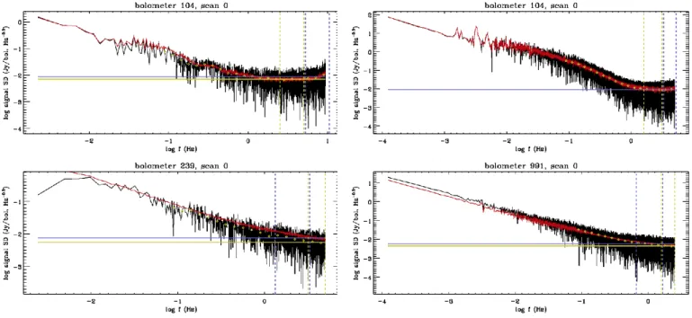
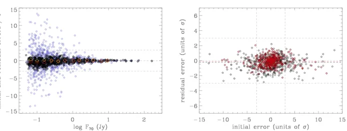
Fig. 1.— Example of determination of the high-frequency noise from spectral densities computed after in-terpolating compact sources and glitches, at the nominal SPIRE sampling rate (top left, from the NGC 6946 250µm observation), at the parallel-mode sampling rate for SPIRE (top right, from the Rosette 250µm ob-servation); and for PACS in nominal mode (bottom left, from the NGC 4559 160µm observation), and in parallel mode for the blue array (bottom right, from the Rosette 70µm observation).SDstands for spectral density, andffor frequency. The vertical lines show the frequency ranges within which the average of the spectral density is computed, and the horizontal lines the derived noise spectral density. The white noise is coded in yellow, and the threshold noise in blue (see Sect. 3.3). The yellow diamonds represent the binned spectral density. The high-frequency noise is computed individually for each bolometer. The red curve shows the average spectral density of all bolometers, for comparison.
Prior to the computation of spectral densities, real high-frequency signal - that may contaminate our noise estimates - is masked in the following way: whenever the absolute difference between the signal at a given time and the signal between one and three time steps later exceeds a given threshold (computed from the dispersion of the absolute differences in the observation), a total interval of six samples around that
time are temporarily masked out. Because the Fourier transform needs continuous time series, the masked samples are then interpolated, and an artificial Gaussian noise is added to the interpolates. The mapping of the signal that has been removed in this way shows that the procedure is effective at removing both bright compact sources and glitches (an example is shown in Fig. 12).
For the removal of drifts, it is necessary to use a second noise quantification that serves to define a threshold for the detection of compact sources, steep brightness gradients and glitches (see Section 3.5.1). For SPIRE, since some pipeline modules using Fourier transforms amplify the high-frequency noise, the spectral densities rise again beyond 5 Hz. To take this into account in our noise threshold, we measure the average noise standard deviation between 5 and 10 Hz. We call this estimate (or the “white noise” estimate if it is larger) the “threshold noise”. Similarly, we measure such a quantity for PACS, between 1.3 and 3 Hz. All the frequency windows are modified in parallel mode, when the sampling rate is lower. Illustrations of the high-frequency noise computation are shown in Fig. 1. After computing the high-frequency noise of all bolometers, in each scan, those with very deviant noise values are masked and not further used.
For PACS, the brightness quantization noise is in some cases a significant fraction of the high-frequency noise. We estimate it in the following way: for each bolometer and each scan, the quantization step qis defined as the minimum brightness where the histogram of|B(ti+1)−B(ti)|, computed on a very fine brightness
grid (excluding zero), is populated,B(ti) being the brightness recorded at theithtime sample. Assuming that
the quantization error is uniformly distributed between 0 andq, the quantization noise variance is thenq2/3. When this term dominates the high-frequency noise (which happened in the early stages of the mission when using a very low gain), it may limit our ability to subtract the low-frequency noise down to acceptable levels.
3.4. Long-timescale drift subtraction
Scan observations do not allow to separate the brightness drifts from the signal on spatial scales similar to or larger than the map size, i.e. on timescales of the order of the scan leg duration of larger. Such drifts, if left uncorrected, may introduce artificial brightness gradients. For thermal drifts, that are usually coherent over the duration of several scan legs or whole scans, these gradients will be perpendicular to the scan direction (see an example in Sect. 5.2.2). The simplest way to remedy this problem is to subtract linear baselines, computed either on a scan basis, or on a scan leg basis, but this requires particular care, in order to keep the baselines immune to real structures that are smaller than the field of view, and to preserve as much as possible brightness gradients that could be real. These baselines in fact cover several distinct instrumental artefacts: the primary component consists of flux calibration offsets, as mentioned above (Sect. 2.3), and the rest comprises the long-timescale component of both the thermal drift and the flicker noise.
We argue that baselines should not assume the form of polynomials of any order higher than 1 (this is an option offered in the pipeline), whenever possible. With an order of 2 or higher, the shape of structures smaller than the field of view is altered, in an uncontrolled way. In Scanamorphos, the subtraction of the drifts on timescales smaller than the field of view crossing time are left to specific modules using the redundancy, and thus operating in a controlled way, such that flux and morphology are conserved.
The baseline-subtraction algorithm described here was implemented specifically for Herschel, and needs to be adapted if scans cannot be sliced into distinct scan legs. We need to distinguish three cate-gories of fields, for which the algorithm will be slightly different. Extragalactic fields are the easier case, because the sky has at most very mild brightness gradients, that are insignificant with respect to the effects of a thermal drift (any field where a flat sky can be isolated from sources belongs to the same category, even if located within the Galaxy). The second case is that of bright Galactic fields (e.g. star formation regions), where sky gradients can become comparable to the artificial gradients induced by the drifts; their separation requires special steps. Finally, another modification to the general algorithm is needed for very small fields, as explained at the end of this section.
Extragalactic or faint fields: First, simple baselines are computed by the process outlined below in points 1 to 3, iterated three times:
1) On a scan basis, we fit a linear function to the signal averaged over all valid bolometers, and subtract it from the signal of each bolometer. In practice, this removes a major part of the average low-frequency noise. This step can modify the general brightness gradient in the scan-perpendicular direction, but not in the scan-parallel direction.
2) On a scan leg basis, one offset (or zero-order baseline) is subtracted for each valid bolometer. This step takes care of flux-calibration offsets, and can also include a very small contribution from the low-frequency noise, since the offsets are allowed to vary from one scan leg to the next. Each offset is determined as the median of the series.
3) At the third iteration, zero-order baselines in step 2 are replaced with linear baselines. A distinction is made between fields with structure extending over scales similar to the map size, and fields where the extended emission is confined to the central part of the map: if the former case applies, then the baselines are constrained such that their average over all valid bolometers reduces to the zeroth order, so that in practice the general brightness gradient is not altered. An example of such a case is a field with strong cirrus emission on one side of the map (see Sect. 5.1.3).
The fits in steps 1 and 3 and the offsets in step 2 are robust, in the sense that a mechanism is in place to iteratively exclude sources from the brightness series, both in the time domain and in the spatial domain. For the latter, a new map is created after each step, and sources above a given threshold are masked; the mask is then transferred to the time domain. The applied brightness threshold is determined automatically, and is chosen so as to avoid masking predominantly the edges, in case significant structure exists outside the central part of the map (see an example in Sect. 5.1.1).
The discrimination between the two types of structure in step 3 is made automatically, and requires no user input. It is based on the same source mask as above, except that the brightness threshold is fixed. The map is divided into a central part (one ninth of the surface area) and the periphery. The fractional area of the source mask located within the central part decides of which case applies: if it is smaller than a given threshold, and if the total area of the mask is significant, then we consider that there is extended emission throughout the map.
4) Once these simple baselines are subtracted, they are refined by using the redundancy in the observation instead of fits (which provide a useful pre-correction but are unphysical). This complementary destriping ensures that the most accurate solution is found, by minimizing the deviations between different bolometers and between successive scans. This is an iterative process using the same source mask as above. At each iteration, and for each scan leg, the difference between the series of each valid bolometer and the series simulated from a reference map (both associated with the same sky coordinates) is computed and fitted by a linear function, and this linear baseline is subtracted from the data; then the map is updated and the process repeated until convergence. The reference map is first built from scans taken in the direction orthogonal to the scan leg under consideration, and then in later iterations from all scans (see below for a detailed explanation).
The destriping algorithm assumes that each scan leg is separated from the next by a spatial offset larger than the FWHM or a few times the FWHM. While this is always true for nominal observations, this condition is not verified for fine scans used for calibration purposes. When processing fine scans, the destriping module should therefore be deactivated.
Galactic or complex bright fields: For observations of such fields, if the relevant option is used (/ galac-tic), the baseline subtraction is modified with the aim to protect as well as possible complex structures of0.3ten extending over much larger scales than the field of view. The modified algorithm is applicable only when sources are bright enough to be visible in the map built from raw data (or rather when only the flux calibration offsets have been subtracted).
1) On a scan basis, linear baselines are replaced with simple offsets, so that the natural brightness gradients of molecular clouds, usually dominant over gradients induced by low-frequency noise, are left intact. The offsets are computed for each valid bolometer as the median of the series, and in practice eliminate the flux calibration offsets.
2) Still on a scan basis, linear baselines are computed by using the redundancy: the difference between the average series of the valid bolometers and the average series simulated from a reference map is computed and fitted by a linear function, and this linear baseline is subtracted from the data; then the map is updated and the process repeated for a total of four times. For each scan, the reference map is built from the scans acquired in the (near-)orthogonal direction only, in the first two iterations. In the last two, once the scans have been rectified, the reference map includes all the scans. Natural gradients are preserved for this reason: when subtracting a linear baseline from a whole scan, only the gradient perpendicular to the scan direction can be modified; any gradient parallel to the scan direction would create a periodic signal (with a period equal to the duration of two scan legs), and would not create any linear component. Any real gradient will be present in both the fitted scan and the reference map, and thus cancelled when subtracting the series simulated from the reference map, before doing the fit. As to the artificial gradients caused by the thermal drift, they are to first order perpendicular to the scan direction (i.e. parallel to the displacement from one scan leg to the next), since low frequencies are dominant. Thus they have a distinct orientation in the fitted scan and in the reference map, when the latter is built from scans acquired at a sufficiently distinct angle: the drift in a given scan will be left intact by the subtraction of the reference series and can be fitted by a
linear function and removed.
3) The destriping is repeated, this time for each bolometer independently, on smaller segments of four scan legs, i.e. at a better time resolution but still ensuring immunity to scan-parallel gradients. The scheme to build the reference map is the same as in step 2.
4) Then, the destriping on a scan leg basis is made in the same way as for extragalactic fields. A source mask is also defined and used in the same way as above in all steps.
Very small fields: For such observations, the destriping and average drift subtraction on small scales become impossible, because there are not enough resolution elements across the map. This can lead to an ill-determined thermal drift, in case it is significantly non-linear, which occasionally happens. To solve this problem, for small fields whose source mask covers a small fraction of the total area, we allow third-order baselines in place of linear baselines (on a scan basis). The order change is however effected only when the new fit is of much better quality than the linear fit, as measured by theχ2value.
3.5. Short-timescale drift subtraction
We now discuss the removal of drifts on timescales shorter than the scan leg duration, which can be derived without any assumptions on the sky structure, contrary to those discussed in the previous section.
3.5.1. Average drift
In a first step, as mentioned in Section 3.1, thermal drifts are considered to be uniform over the whole array; any component that differs from the average is treated in the second step, as part of the uncorrelated drifts. We thus have to determine a single series for the thermal noise.
For each pixel of the coarse grid (Sect. 3.2), all the samples recorded while the beam center lies within this pixel are searched; an efficient IDL function is used to perform this task quickly and store the sample indices beforehand. Then, the samples are divided into separate bolometer crossings, for each of which the brightness mean and the brightness mean absolute deviation are computed, and to each of which an average time is attached. Bolometers scanning only pixel corners, with insufficient statistics, are discarded.
At this point, the presence of a compact source, a steep brightness gradient, or an abnormal level of high-frequency noise within the pixel, is tested in a straightforward way: if the mean absolute deviation of a bolometer crossing is below the average threshold noise of this bolometer (defined in Section 3.3), then it is deemed suitable for drift determination; otherwise, the assumption of a uniform astronomical signal is not valid. We then distinguish two cases: 1) If more than 70 to 80% of the bolometer crossings are suitable for drift computation, then they are effectively used, and only those bolometer crossings with an elevated mean absolute deviation are discarded. 2) In the opposite case, then a significant portion of the coarse pixel area is assumed to contain non-uniform signal, and all the bolometer crossings are discarded. If the sampling rate
allows the statistics to remain sufficient at smaller scales, then the algorithm switches to a finer spatial grid, to which the same test is applied; if the test is again negative, all the bolometer crossings are again rejected. The measured brightness difference between each pair of suitable bolometer crossings is in principle equal to the difference of the drifts between the two sampled times. Calling the first bolometerbi, crossing
the pixelpat the average timet1, and the second bolometerbj, crossingpat the average timet2,
δ(t1,t2)=R(t1,bi)−R(t2,bj) (3)
= D¯(t1)−D¯(t2)+Dbi(t1)−Dbj(t2)+HF(t1,bi)−HF(t2,bj)
The S(p) term in Equ. 2 cancels because the astronomical signal is assumed both invariant in time and uniform within p, making the different trajectories ofbi andbjwithin pirrelevant. The software is in fact
able to cope with mild non-uniformity withinp, since the current map is used to cancel, whenever possible, brightness differences purely caused by small pointing differences, as explained in Section 3.5.4. Then, by linear interpolation,δ(tc1,tc2) (on the coarse time grid defined in Section 3.2) is obtained fromδ(t1,t2) .
Each termδ(tc1,tc2) is stored in a matrix where the first dimension represents the smaller of the two
times, and the second dimension the larger. Drift differences are coadded in this matrix as they are computed, regardless of the position on the sky or the bolometers involved. Their weights, inversely proportional to the square white noise of each bolometer, are stored symmetrically across the matrix diagonal. This ensures, together with the use of a coarse time grid adapted to the minimum drifts timescale, that memory usage is minimized.
One obtains by coadditions
δ(tc1,tc2)=D¯(tc1)−D¯(tc2)+WMp,i,j[Dbi(tc1)−Dbj(tc2)] (4)
where WM designates the weighted mean and the sum runs on all pixels p and all pairs of bolometer indices (i, j) such that bi is crossing p at time tc1 and bj is crossing the same pixel p at time tc2. The
high-frequency noise term rapidly vanishes and, given that the individual drifts are all independent of each other, the WM term above also becomes negligible if the redundancy is sufficient. Taking as an example the 70µm PACS observations of the Rosette nebula discussed in Section 5.2.2, made of 2 scans in parallel mode at the scan speed of 2000/s (thus with relatively low redundancy), the median number of contributing bolometer crossings for a given (tc1,tc2) time pair isNcoadd '380 , with a very large spread. The residuals
of the WM term inδ(tc1,tc2) are thus of the order of √ 1
Ncoadd
'5% of the average amplitude of the individual drifts (which is larger than the amplitude of the average drift at any given frequency for PACS). However, the average drift series is obtained from the δ(tc1,tc2) terms in a complicated fashion (see next section),
involving many more coadditions. Although a rigorous analytic estimate cannot be made, the final residuals due to the WM terms are very small compared with the amplitude of the average drift, as proven by the simulations in Section 4. Let us remark that the probability law of the individual drifts does not have to be assumed Gaussian; it only has to be symmetric about zero. Finally,δ(tc1,tc2)' D¯(tc1)−D¯(tc2).
Once all pixels have been covered, the matrix is read so as to restore from the drift differences the average drift series (see next section), that is subtracted from the signal series of each bolometer. Since it is
impossible to define the absolute zero of the drift, it is previously offset so that its time average is null. Then a new map is projected.
This process is iterated until convergence, which is reached when the drift amplitude has become smaller than the white noise level for most bolometers. Here, the amplitude of the drift is defined as three times its standard deviation.
3.5.2. From drift differences to the absolute drift series
The conversion of the drift differences matrix to the absolute drift series is not trivial. First, the matrix is scanned several times in each direction, progressively populating the drift series. One entry time is chosen and arbitrarily assigned a null drift. Then, each drift difference between two times of which one has already an entry in the drift series is used to assign an absolute drift to the second time index. At the same time as the drift series is built, a corresponding weight series is computed, and used to weight appropriately the drifts as they are coadded. The matrix is scanned until the drift series converges.
This process does not provide a unique solution. Let us assume that the average drift ¯D(t) is replaced with ¯D(t) +E(t), where E(t) is an excess drift, such that the projection of this series produces the same map for each successive scan (i.e. E(t) is an oscillatory function, with a period equal to that of the spatial coordinates, just like the average true sky series). Then theδ(t1,t2) term in Equation 3 is unchanged, because
it is computed within a single pixelp, whereE(t1) andE(t2) take the same value. The drift series obtained by scanning the drift differences matrix is thus the superposition of the true drift series and an oscillatory component. The average drift has no reason to repeat itself exactly in successive scans. We thus extract this periodic component from the average drift and remove it, before subtracting the average drift from the data. This is achieved by first mapping the average drift for each scan separately, and extracting the component common to all these maps, that we call the excess drift. Then, the series of the excess drift is simulated from its map, and finally subtracted from the original drift.
We now briefly explain the method used to extract the excess drift from the drift maps. This method has to provide reliable results even when the observation is composed of only two scans, i.e. only one period of the excess drift. We exploit the fact that, by definition, the excess drift varies on much longer timescales than the true drift (that varies on timescales shorter than the duration of a scan leg). This implies that the spatial variations of the excess drift in the drift maps are much smoother than those of the true drift. For each drift map (one per scan), a map of the local variance is computed (using as zero moment a boxcar-averaged version of the drift map). Then the excess drift map is defined as the weighted average of all the drift maps, the weight for each one being the inverse variance map. Obviously, the error on the excess average drift will go down as the number of scans increases. When a large number of scans are combined, the excess drift map is simply defined as the median of all the drift maps.
3.5.3. Individual drifts
In a second step, the individual drifts are removed. At this stage, by definition, the drift affecting the average signal of all valid bolometers should be close to zero at all times. Using the same scheme as previously and protecting non-uniform signal in the same way, this allows us to equate the drift of an individual bolometer to the difference between its signal and the average bolometer signal, at any given position on the sky. This average signal is weighted by the inverse square white noise of each bolometer, and considered to represent the intrinsic sky brightness. Calling the bolometer of interestbi, crossing a pixel pat timet, andbjall the valid bolometers crossing pat timestk:
∆(t,bi)=R(t,bi)−WMj[R(tk,bj)]
=D¯(t)+Dbi(t)+HF(t,bi)−WMj[ ¯D(tk)+Dbj(tk)] (5) By the same argument as before, theS(p) term in Equ. 2 cancels and the high-frequency noise term of the weighted mean vanishes. Since the average drift has been subtracted beforehand, and interpolating linearly on the coarse time grid, we have
∆(tc,bi)=Dbi(tc)+HF(tc,bi)−W Mj[Dbj(tck)]. (6) Given sufficient redundancy, the rightmost term once again becomes negligible because the individual drifts are uncorrelated. Taking the same example of the Rosette nebula as above (Sect. 3.5.1), the average redundancy isNcoadd'650 bolometer crossings per coarse pixel (with sizels=4.5 FWHM). The residuals
of the WM term are thus of the order of √ 1
Ncoadd
' 4% of the average amplitude of the individual drifts for this particular example. The other examples in Table 1 have much higher redundancies, thus lower residuals. Finally, one obtains ∆(tc,bi) ' Dbi(tc)+HF(tc,bi). We can neglect the high-frequency noise term (binned on the coarse time grid), as long as the drift dominates.
A value of zero is assigned to the drifts over the time steps when they are undefined (corresponding to compact sources, steep gradients and glitches). At each iteration, a residual map – equal to the difference between the map produced at the previous step and the current map – allows to immediately assess whether compact sources have been altered or not, and by which percentage. The interpretation of the residual map is however not straightforward, since artefacts at the location of bright sources can result from small pointing and gain errors. Intermediate results can also be visualized in the form of selected signal and drift series. The convergence criterion is the same as for the average drift.
Although combining two scans or more is desirable, this algorithm is able to remove some of the low-frequency noise even when only one scan is available. This allows data quality and depth to be assessed on a single-scan basis before multi-scan observations are fully completed.
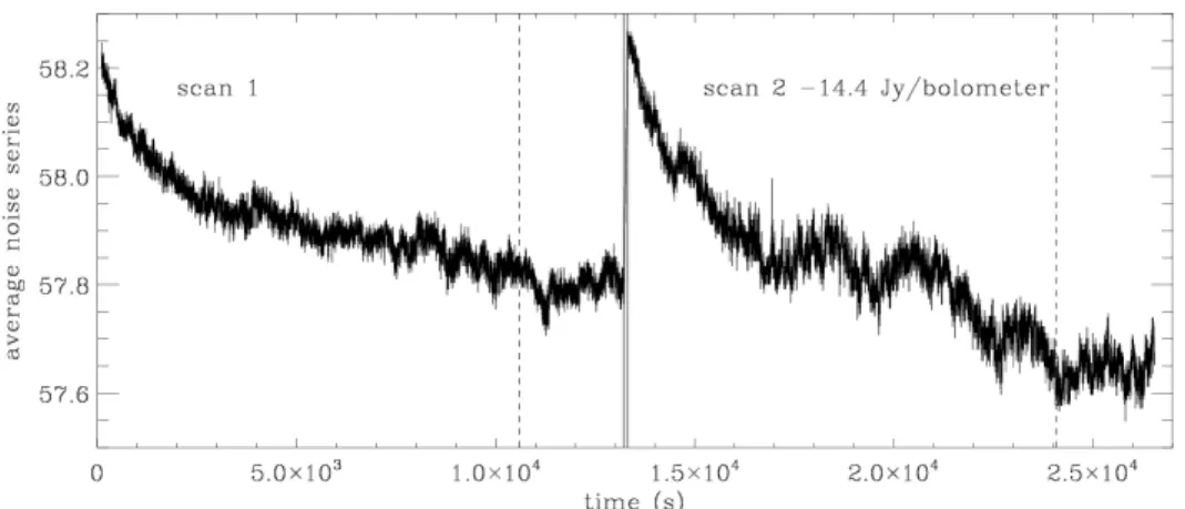
The noise spectral density of each bolometer, computed from the noise series derived by the software, is an optional output, and can be compared with the noise spectral density that is part of the pipeline calibration products, allowing an independent test of the assumptions on the noise used by the pipeline. An example obtained from the processing of flight data is shown below (Sect. 5.1.2).
3.5.4. Correction for pointing differences within the stability length
As mentioned in Section 3.5.1, for the computation of both the average drift and the individual drifts, we have to cope with mild gradients within the stability length, i.e. non-uniformities of the signal that are too shallow to produce a significant increase of the mean absolute deviations of the bolometer crossings. Given that each bolometer follows a different trajectory within a coarse pixel, and since the stability length is large compared with the angular resolution, especially for PACS data, these mild gradients may contam-inate the drift estimate if ignored. The strategy to follow depends on the prominence of the low-frequency noise: in SPIRE data, where the signal is never dominated by the short-timescale drifts, the correction for pointing differences is always applied; but in PACS data, where the short-timescale drifts are of much higher amplitude, the correction should not be applied in all circumstances, because it might be dominated by noise rather than real spatial variations.
In each coarse pixel where no compact source was detected, we have to decide whether the correction for pointing differences will be applied to all the bolometer crossings, or not at all. We consider two sets of series: the uncorrected series of recorded samplesR(t,bi), and the series corrected for pointing differences
˜
R(t,bi) = R(t,bi)− M(p(t,bi)), where M(p(t,bi)) is the signal of bolometer bi simulated from the current
map, built on a fine grid of pixels p much smaller than the stability length. Brightness gradients, which affect all bolometers in the same way, are present in bothR(t,bi) andM(p(t,bi)), and can thus be cancelled
by computing the difference. If the signal within the coarse pixel is not dominated by the drifts but by sources, thenM(p(t,bi)) is a fair representation of the sky emission; otherwise, it cannot be used to subtract
gradients.
For SPIRE,R(t,bi) is always replaced with ˜R(t,bi) before computing the drifts. For PACS, to choose
between the two alternatives, we try to quantify the non-uniformity of the fine map at the location of the coarse pixel, and compare it with the expected white noiseΣat the same location (estimated from the square root of the inverse weight map). If the local brightness is more than a few timesΣabove a local background or above the global background, then the pointing correction is applied; in the opposite case, the signal is deemed perfectly uniform and the pointing correction is not applied.
3.5.5. Time resolution for the individual drifts
For PACS data, we have serendipitously found that the accuracy of the individual drifts could be improved by first doing the correction on much longer timescales than allowed by the stability length (Sect. 3.2), and then gradually increasing the time resolution until reaching the minimum drift timescale. At the first iteration, the size of the coarse pixel is left unchanged, but the drift correction is binned into time intervals that are 27 times larger than the stepTcof the coarse time grid. The time resolution is increased by
a factor of 3 at each of the following three iterations.
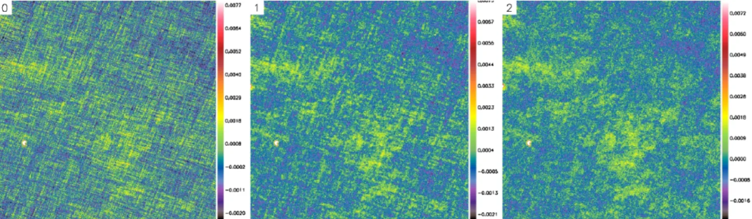
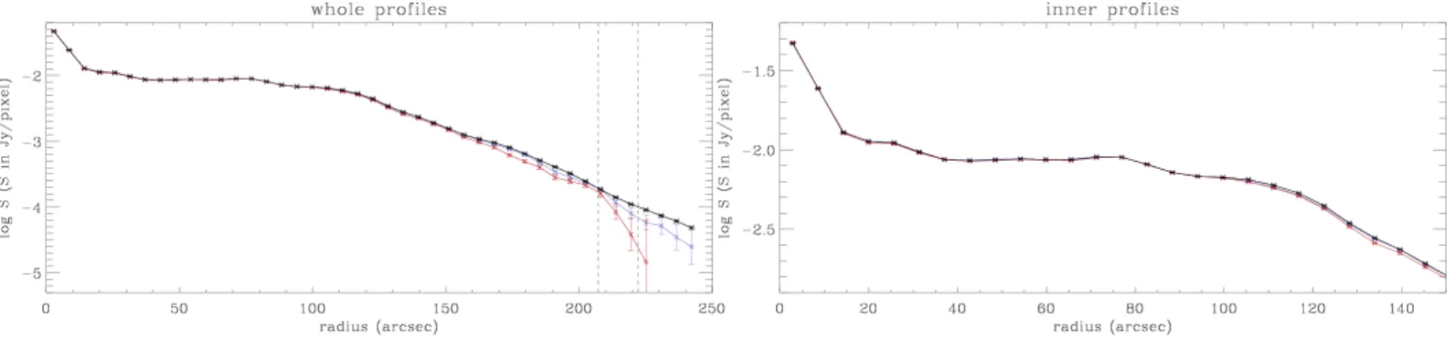
This modification greatly reduces the residual noise in diffuse areas of large PACS maps, and the scan pattern becomes indiscernible, as shown in Figure 2. We conjecture the following reason. The algorithm
relies on the assumption that the coaddition of the individual drifts affecting all the bolometer crossings (the rightmost term in Equ. 6) is close to zero, because the drifts are uncorrelated. This assumption may not be perfectly verified, causing a residual noise. Averaging a great number of drift values within a large time interval will average out this noise. Since the drifts have more power at lower frequencies, the first iteration with a time step of 27×Tcremoves a major part of them, and it becomes easier to verify our initial
assumption on smaller and smaller timescales.
Fig. 2.— A subfield of the HEVICS survey (Davies et al. 2010), about 2.2 degrees on a side, from 160-micron data processed in three different ways: 0) No drifts (on timescales shorter than the scan leg duration) have been subtracted. 1) The iterations to subtract the individual drifts all have the minimum time stepTc.
2) They have successive time steps of 27×Tc, 9×Tc, 3×Tc andTc. The display emphasizes very diffuse
structures.
3.6. Detection of other artefacts
3.6.1. Masking of brightness discontinuities
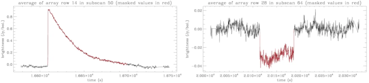
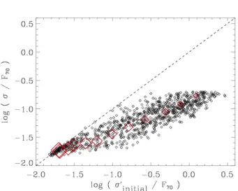
During tests conducted on various PACS datasets, the presence of brightness discontinuities affecting whole array rows (blocks of 16 pixels) or, less frequently, individual bolometers, was noticed. These arte-facts are caused by glitches, and also often by electronic instabilities in the multiplexing circuit, that may come and go during the course of an observation. They are currently not corrected for in the pipeline, but they can impact the quality of the maps, leaving bright or dark bands. Since they are high-frequency features followed by a slow decay or a plateau, they can be corrected neither by the deglitching modules nor by the drift subtraction modules. Examples of such artefacts are shown in Fig. 3.
We have therefore developed a module to detect these discontinuities and mask the subsequent frames. This module handles the average series of each 16-pixel block, and then the series of individual bolometers of each block. Spatial information is used jointly with temporal information, making the detections more robust and more sensitive: the series simulated from the current map are subtracted from the observed series. Candidate discontinuities are found whenever the absolute difference between the signal at a given
time and the signal three time steps later exceeds a predefined threshold. A candidate is confirmed if it can be unambiguously distinguished from a real brightness variation caused by a compact source or a steep gradient of emission. To this effect, the median brightness and the standard deviation of the series are computed within four time windows, on each side of the potential discontinuity. A diagnostic is made based on these values to rule out compact sources. In addition, to avoid false detections caused by steep gradients (such as present in molecular clouds or edge-on disks), this diagnostic is combined with a thresholding based on the dispersion of the signal in the neighbourhood of each detection. If the candidate is confirmed, subsequent frames of the array row are masked, until the end of the scan leg or until their average brightness gets back to the pre-discontinuity brightness to within the white noise level.
Fig. 3.— Example of brightness discontinuities in PACS data (left: caused by a glitch; right: caused by an electronic instability). The average series of an array row (16 contiguous pixels) is plotted over a particular scan leg. All the bolometers in the row are affected by the artefact. Overplotted in red are the data that have been masked by the dicontinuity detection module.
3.6.2. Masking of glitches
The software includes the capability to filter glitches remaining after the pipeline processing, whether a deglitching module was run in HIPE or not. They are not interpolated but all affected samples are per-manently masked. The detection of glitches shares a portion of its algorithm with modules in charge of computing both the high-frequency noise, and the average and individual brightness drifts. For this reason, the deglitching task is embedded within these modules, and thus split into several steps.
The computation of the frequency noise from the spectral densities is made after replacing high-frequency contaminants (both compact sources and glitches) with interpolates (see Sect. 3.3). The samples that are filtered in this process are further examined to separate glitches from real signal. Glitches must simultaneously show a significant deviation from the median signal at their location, and exceed three or four times this reference signal in absolute value (to avoid flagging the sidelobes of a bright compact source). An example of the effectiveness of this approach is shown in Sect. 5.1.2. This is especially useful for SPIRE, because the pipeline includes Fourier-filtering tasks, that can strongly amplify undetected glitches in some instances, as shown in Fig. 15. This problem may be alleviated by using second-level deglitching, or can be
dealt with byScanamorphos.
The computation of the brightness drifts makes use of some simple statistics on bolometer crossings, in order to filter out those with large standard deviations, to protect compact sources (see Sect. 3.5.1). These statistics can also be used to detect glitches. The separation between glitches and real signal with a strong brightness gradient is made by estimating gradients and standard deviations just before and just after the suspect samples. This second deglitching is bypassed when the stability length, determining the pixel size of the grid used for drifts computation, is large compared with the beam FWHM.
3.6.3. Detection of transient sources
Asteroids or other transient sources, that are present at a given location in one scan but have moved or vanished in the other scans, are also detected. The method used to detect them and distinguish them from glitches is based on the fact that they produce a coherent signal for all bolometers as the latter cross the source, while glitches do not. They are dealt with at the same time as glitches in step 7 of Section 3.1. They will thus be ignored if the deglitching is deactivated.
If asteroids are detected, a transient-signal map is produced at the end of the processing, using the same spatial grid as the other final maps. In this map, only the affected portions of the bolometer series are projected, and not those when the bolometers were not illuminated by the asteroids. In this way, it is possible to locate them and to obtain an estimate of their true brightness, whereas they appear dimmer in the nominal signal map (if they are present in one of two scans at a given position, their brightness will be roughly divided by two).
3.7. Projection
At the end of the processing, a final projection produces a sky map, a weight map, an error map and a low-frequency noise map, stored together in a FITS data cube. The low-frequency noise map includes the sum of the drifts subtracted at each step. The signal is weighted by the inverse square white noise of each bolometer. The gnomonic projection is used.
The brightness unit is different for both instruments. The flux calibration of SPIRE is valid for point sources, and voltages are converted to Jy per beam by the pipeline. To obtain extended-source flux calibra-tion, the maps have to be divided by the average beam area. Since the associated uncertainties are larger than those of the point-source flux calibration, and since beam areas may continue to be refined in the future, it is best to apply this correction outside the map-making software. SPIRE maps produced byScanamorphos
are thus in Jy per beam. For PACS, the data are initially in Jy per array pixel, and are converted to Jy per map pixel byScanamorphos. The default pixel size, approximately one fourth of the FWHM, better sam-ples the point response function (PRF) than that recommended for the projection within the SPIRE pipeline (between 0.33 and 0.4 times the FWHM, depending on the wavelength).
In the SPIRE pipeline, each sample is projected entirely to the closest pixel. Since pixel sizes are a large fraction of the FWHM, this method introduces a bias between the beam center and the projection center. This bias varies as a function of the source position relative to the pixel grid, and is up toa/√2, whereais the pixel size. We use instead a projection method akin to the drizzling technique (Fruchter & Hook 2002), where the imprint of each sample on the map is a uniform disk of the same area as the default pixel for the final projection (i.e. FWHM2/16), and of the same center as the beam. This method does not introduce any bias in the projection center, and reduces the standard deviation of the sky with respect to HIPE maps, by a significant amount (in some configurations, by more than 30% if the low-frequency noise has been perfectly removed). This comes at the expense of a slightly larger PRF: the FWHM is increased by 1.5% (and the area by 3%). Note that the projection affects only the PRF profile, and has no incidence on the beam area to be used to convert units of Jy per beam to units of Jy per pixel.
For PACS, our projection also uses the simplifying assumption of axisymmetric bolometers, whereas the bolometers in reality consist of square pixels (with small distortions). The bolometer imprint is chosen to have a slightly smaller area than the true array pixel, just like in the drizzle projection. It is in princi-ple possible to save the corrected signal series and to perform the final projection within the pipeline for optimum accuracy, but the PRF has not been found to be appreciably modified by our projection.
3.7.1. Weight and error maps
The weight map is defined differently from the coverage map produced by HIPE. It is built by coadding the weights, using the same projection as the sky map, and is normalized by the average of the weights (the average is computed over all the valid bolometers and all the scans). For the nominal data acquired at constant scan speed, the weights are defined as the inverse square white noise values. For turnaround data, acquired at lower or higher scan speed, these weights are decreased so that edges of the map, where both nominal and turnaround data can contribute, are not dominated by low-velocity data.
The error map produced byScanamorphosis defined as the error on the mean brightness in each pixel. It is built using the (unbiased) weighted variance instead of the simple unweighted variance, since weights are used for the projection of the sky map. It does not include any errors associated with the different pro-cessing steps in the pipeline, because these errors are currently not propagated. It should however be useful to estimate the random photometric errors, and to filter glitches that may have escaped detection. Elevated errors will be found both at the location of bright compact sources and in pixels affected by unmasked glitches.
Artefacts that may remain when the redundancy is low can also be spotted by comparing the signal map with the “clean” map in the fifth plane of the cube, that is weighted to exclude noisy scans in each pixel. The latter map is produced in general only when there are two or three scans, and is intended as a diagnostic for the presence of artefacts in the signal map (features that are absent in the ”clean” map). It should not be used for scientific purposes, only as an aid to mask bad data.
3.8. Spatial slicing
For deep observations of wide fields, the software has the ability to slice the data into several partially overlapping fields, in order to minimize memory and computing time usage. This is suitable for observations without very extended bright emission, since it cannot be ensured that extended sources are covered by a single sub-field. For each sub-field, all the available redundancy is used as if it were an entire observation. In the end, the different maps are stitched by matching the brightness levels in the parts of the overlap areas where coverage is nominal.
In the various tests that we conducted, we have not found it necessary to reduce the data volume when the processing was done on a machine with a total memory of 48 Gb, but this functionality was used for some deep observations processed on a machine with a total memory of 8 Gb.
It may sometimes be desirable to do the processing in several spatial blocks, even though the available memory is sufficient to process the entire observation at once. If the observation is long and the subtraction of the short-timescale average drift is required, limitations on the size of the drift differences matrix can make the minimum timescale for the average drift computation longer than that for the individual drifts computation. It is then possible to increase the time resolution of the average drift by decreasing the data volume, which is achieved by slicing the field of view into several blocks.
4. Simulations of PACS observations
We now quantify the effect of the processing withScanamorphoson the data, using simulations. The instrumental artefacts of PACS are more difficult to remove than those of SPIRE, chiefly because the low-frequency noise has a much greater amplitude with respect to both the signal and the high-low-frequency noise, and because the stability lengths are greater with respect to the FWHM (Sect. 3.2). Additional complexi