Efficient Simulations in Finance

(1)

Halis Sak

Efficient Simulations in Finance

Working Paper

Original Citation:

Sak, Halis (2008) Efficient Simulations in Finance. Research Report Series / Department of Statistics and Mathematics, 71. Department of Statistics and Mathematics, WU Vienna University of Economics and Business, Vienna.

This version is available at: http://epub.wu.ac.at/1068/ Available in ePubWU_{: September 2008}

ePubWU_{, the institutional repository of the WU Vienna University of Economics and Business, is}

provided by the University Library and the IT-Services. The aim is to enable open access to the scholarly output of the WU.

(2)

Halis Sak

Department of Statistics and Mathematics Wirtschaftsuniversit ¨at Wien

Research Report Series

Report 71

September 2008

(3)

by Halis Sak

B.Sc., in Mechanical Engineering, Middle East Technical University, 2000 M.Sc., in Industrial Engineering, Bo˘gazi¸ci University, 2003

Submitted to the Institute for Graduate Studies in Science and Engineering in partial fulfillment of

the requirements for the degree of Doctor of Philosophy

Graduate Program in Industrial Engineering Bo˘gazi¸ci University

(4)

EFFICIENT SIMULATIONS IN FINANCE

APPROVED BY:

Assoc. Prof. Wolfgang H¨ormann . . . . (Thesis Supervisor)

Assoc. Prof. Necati Aras . . . .

Prof. Refik G¨ull¨u . . . .

Assoc. Prof. Josef Leydold . . . .

Prof. S¨uleyman ¨Ozekici . . . .

(5)

ACKNOWLEDGEMENTS

I am grateful to my advisor, Assoc. Prof. Wolfgang Hörmann for introducing me to the field of simulation. Without his guidance and patience, I would have probably being lost in this study. I am also grateful to the members of examining committee, Prof. Süleyman Özekici and Prof. Refik Güllü, for their helpful comments during my study. It was a great pleasure for me to do my research under supervision of these three researchers.

I had been working as a teaching assistant at ˙Istanbul Kültür University during most of the time of my thesis study. I want to thank Prof. Tülin Aktin for her support as an employer during this period of time.

I have been partially supported from the scholarship program B˙IDEP 2211 of The Scientific and Technological Research Council of Turkey (T ¨UB˙ITAK) during my research. Many thanks to them for giving the feeling of financially secure for just doing what we meant to do.

I have been working as a research assistant in a project for four months in the department of Statistics and Mathematics, Vienna University of Economics and Busi-ness Administration. I am grateful to Prof. Josef Leydold, Prof. Kurt Hornik, Karin Haupt, Stefan Theußl and others for their support and hospitality during my time in Vienna.

I want to thank my brothers, parents and to all who really care about me. Finally, I want to specifically thank Ha¸sim Sak and Sibel Tombaz for their support and love.

(6)

ABSTRACT

EFFICIENT SIMULATIONS IN FINANCE

Measuring the risk of a credit portfolio is a challenge for financial institutions because of the regulations brought by the Basel Committee. In recent years lots of models and state-of-the-art methods, which utilize Monte Carlo simulation, were pro-posed to solve this problem. In most of the models factors are used to account for the correlations between obligors. We concentrate on the the normal copula model, which assumes multivariate normality of the factors. Computation of value at risk (VaR) and expected shortfall (ES) for realistic credit portfolio models is subtle, since, (i) there is dependency throughout the portfolio; (ii) an efficient method is required to compute tail loss probabilities and conditional expectations at multiple points simultaneously. This is why Monte Carlo simulation must be improved by variance reduction tech-niques such as importance sampling (IS). Optimal IS probabilities are computed and compared with the “asymptotically optimal” probabilities for credit portfolios consist-ing of groups of independent obligors. Then, a new method is developed for simulatconsist-ing tail loss probabilities and conditional expectations for a standard credit risk portfolio. The new method is an integration of IS with inner replications using geometric short-cut for dependent obligors in a normal copula framework. Numerical results show that the new method is better than naive simulation for computing tail loss probabilities and conditional expectations at a single x and VaR value. Furthermore, it is clearly better than two-step IS in a single simulation to compute tail loss probabilities and conditional expectations at multiplexand VaR values. Then, the performance of outer IS strategies, which consider only shifting the mean of the systematic risk factors of realistic credit risk portfolios are evaluated. Finally, it is shown that compared to the standard t statistic a skewness-correction method of Peter Hall is a simple and more accurate alternative for constructing confidence intervals.

(7)

¨

OZET

VER˙IML˙I F˙INANSAL S˙IM ¨

ULASYONLAR

Basel komitesinin düzenlemeleri finansal enstitüler i¸cin zor bir i¸s olan kredi portföy riskinin hesaplanmasını zorunlu kılar. Son yıllarda bir ¸cok model ve Monte Carlo simülasyonunu kullanan metodlar geli¸stirilmi¸stir. Bu modellerin ¸co˘gunda yükümlüler arası korrelasyonu sa˘glamak i¸cin faktörler kullanılır. Biz ¸cok-faktörlü normalli˘gin kabul edildi˘gi normal kapula modeli üzerinde yo˘gunla¸sırız. Ger¸cekci kredi potföy modelleri i¸cin riskteki de˘ger (VaR) ve beklenen kuyruk kaybı (ES) hesaplanması kompleks bir i¸stir, ¸cünkü; (i) portföy i¸cinde ba˘gımlılık vardır; (ii) kuyruk kayıp olasılıklarını ve ¸sartlı beklentileri ¸coklu noktalarda aynı anda verebilecek verimli bir metoda gereksinim duyu-lur. Bu yüzden Monte Carlo simülasyonu önemli örnekleme (IS) gibi varyasyon azaltma teknikleri ile geli¸stirilmelidir. Ba˘gımsız ve kü¸cük guruplara bölünebilen yükümlülerden olu¸san kredi portföyleri i¸cin en iyi IS olasılıkları hesaplanır ve bunlar “en iyi asim-totik” olasılıklarla kar¸sıla¸stırılır. Daha sonra standart kredi portföyleri i¸cin kuyruk kayıp olasılıklarını ve ¸sartlı beklentileri simüle edecek yeni bir metod geli¸stirilir. Yeni metod normal kopula kapsamındaki ba˘gımlı yükümlüler i¸cin IS’in geometrik kısa yolu kullananan i¸csel replikasyonlarla birle¸simidir. Numeriksel sonu¸clar, yeni metodun tek bir x ve VaR de˘geri i¸cin standart simülasyondan daha iyi oldu˘gunu ortaya koyar. Buna ek olarak, tek bir simülasyonda birden fazla x ve VaR de˘gerleri i¸cin kuyruk kayıp olasılıklarının ve ¸sartlı beklentilerinin hesaplanmasında iki-a¸samalı IS’den a¸cık bir ¸sekilde daha iyidir. Daha sonra, ger¸cek¸ci kredi portföyleri üzerinde sadece sistematik risk faktörlerinin ortalamasını arttıran dı¸ssal IS stratejileri incelenir. En sonunda, stan-dart t istatisti˘giyle kar¸sıla¸stırıldı˘gında Peter Hall’un yamukluk düzeltme metodunun güven aralı˘gı olu¸sturulmasında kolay ve daha kesin bir alternatif oldu˘gu gösterilir.

(8)

LIST OF FIGURES

Figure 2.1. Tail loss probability computation using exponential twisting for independent obligors. . . 11

Figure 2.2. Tail loss probability computation using two-step IS of [13] for de-pendent obligors. . . 13

Figure 3.1. Naive simulation algorithm for P(L > x) (one obligor case) . . . . 17

Figure 3.2. IS algorithm for P(L > x) (one obligor case) . . . 17

Figure 3.3. Naive simulation algorithm for E[L|L > x] (one obligor case) . . . 19

Figure 3.4. IS algorithm for E[L|L > x] (one obligor case) . . . 19

Figure 3.5. Naive simulation algorithm forP(L > x) (two independent obligors case) . . . 21

Figure 3.6. IS algorithm for P(L > x) (two independent obligors case) . . . . 21

Figure 3.7. Naive simulation algorithm forE[L|L > x] (two independent oblig-ors case) . . . 25

Figure 3.8. IS algorithm for E[L|L > x] (two independent obligors case) . . . 26

Figure 3.9. Naive simulation algorithm forP(L > x) (One homogeneous group of obligors case) . . . 29

(11)

Figure 3.11. Naive simulation algorithm for E[L|L > x] (One homogeneous group of obligors case) . . . 31

Figure 3.12. IS algorithm for E[L|L > x] (One homogeneous group of obligors case) . . . 32

Figure 3.13. Naive simulation algorithm forP(L > x) (Two homogeneous groups of obligors case) . . . 34

Figure 3.14. IS algorithm for P(L > x) (Two homogeneous groups of obligors case) . . . 34

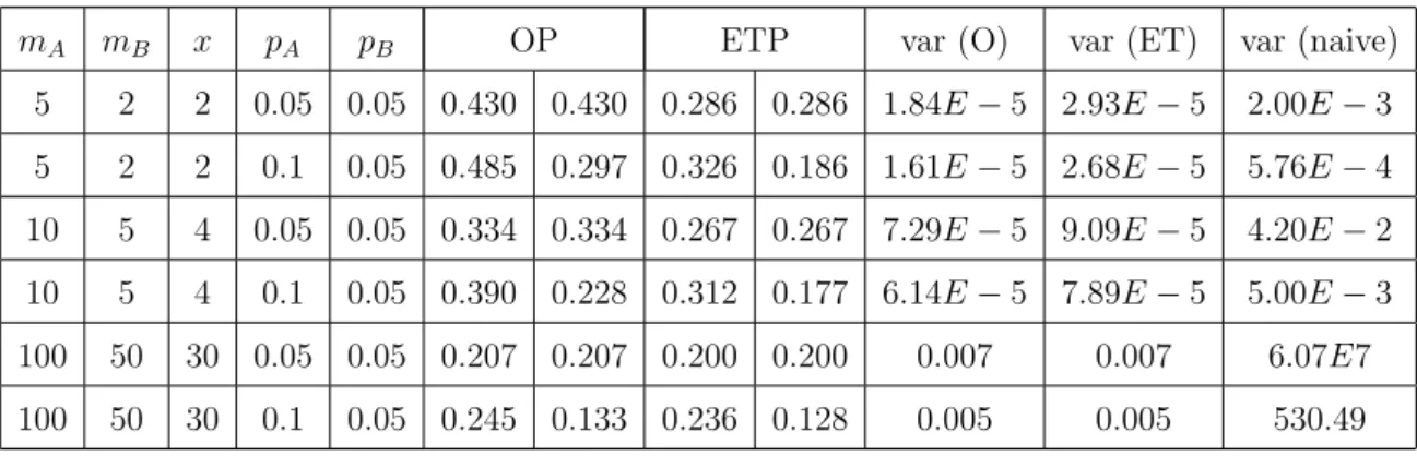
Figure 3.15. Optimal and exponential twisting [13] probabilities and correspond-ing variances for pA= 0.05, pB = 0.05, mA = 5, mB = 2 and x= 2 in computing P(L > x). . . 36

Figure 3.16. Optimal and exponential twisting [13] probabilities and correspond-ing variances for pA = 0.1, pB = 0.05, mA = 5, mB = 2 and x = 2 in computing P(L > x). . . 37

Figure 3.17. Optimal and exponential twisting [13] probabilities and correspond-ing variances forpA= 0.05, pB = 0.05, mA= 10, mB= 5 and x= 4 in computing P(L > x). . . 37

Figure 3.18. Optimal and exponential twisting [13] probabilities and correspond-ing variances for pA= 0.1, pB = 0.05, mA = 10, mB = 5 and x= 4 in computing P(L > x). . . 38

Figure 3.19. Optimal and exponential twisting [13] probabilities and correspond-ing variances for pA = 0.05, pB = 0.05, mA = 100, mB = 50 and x= 30 in computingP(L > x). . . 38

(12)

Figure 3.20. Optimal and exponential twisting [13] probabilities and correspond-ing variances for pA = 0.1, pB = 0.05, mA = 100, mB = 50 and x= 30 in computingP(L > x). . . 39

Figure 3.21. Naive simulation algorithm for E[L|L > x] (Two homogeneous group of obligors case) . . . 40

Figure 3.22. IS algorithm for E[L|L > x] (Two homogeneous group of obligors case) . . . 40

Figure 3.23. Optimal and exponential twisting [13] probabilities and correspond-ing variances for pA= 0.05, pB = 0.05, mA = 5, mB = 2 and x= 2 in computing E[L|L > x]. . . 42

Figure 3.24. Optimal and exponential twisting [13] probabilities and correspond-ing variances for pA = 0.1, pB = 0.05, mA = 5, mB = 2 and x = 2 in computing E[L|L > x]. . . 43

Figure 3.25. Optimal and exponential twisting [13] probabilities and correspond-ing variances forpA= 0.05, pB = 0.05, mA= 10, mB= 5 and x= 4 in computing E[L|L > x]. . . 43

Figure 3.26. Optimal and exponential twisting [13] probabilities and correspond-ing variances for pA= 0.1, pB = 0.05, mA = 10, mB = 5 and x= 4 in computing E[L|L > x]. . . 44

Figure 3.27. Optimal and exponential twisting [13] probabilities and correspond-ing variances for pA = 0.05, pB = 0.05, mA = 100, mB = 50 and x= 30 in computingE[L|L > x]. . . 44

(13)

Figure 3.28. Optimal and exponential twisting [13] probabilities and correspond-ing variances for pA = 0.1, pB = 0.05, mA = 100, mB = 50 and x= 30 in computingE[L|L > x]. . . 45

Figure 4.1. Tail loss probability computation using naive simulation for inde-pendent obligors. . . 52

Figure 4.2. Geometric shortcut in generating default indicators . . . 53

Figure 4.3. Tail loss probability simulation using the geometric shortcut for independent obligors. . . 54

Figure 4.4. Tail loss probability computation using naive simulation for depen-dent obligors. . . 55

Figure 4.5. Inner replications using geometric shortcut in generating default indicators . . . 56

Figure 4.6. Tail loss probability simulation using inner replications using the geometric shortcut for dependent obligors. . . 57

Figure 4.7. Tail loss probability simulation using integration of IS with inner replications using the geometric shortcut for dependent obligors. . 59

Figure 4.8. Naive simulation for computing ES for dependent obligors. . . 60

Figure 4.9. ES simulation using integration of IS with inner replications using the geometric shortcut for dependent obligors. . . 62

Figure 4.10. Comparison of new method with IS in estimating tail loss proba-bilities in the 10-factor model using 1,000 replications. . . 70

(14)

Figure 4.11. Comparison of new method with IS in estimating expected shortfall in the 10-factor model using 10,000 replications. . . 71

(15)

LIST OF TABLES

Table 3.1. Portfolio composition (one obligor case) . . . 16

Table 3.2. Loss Distribution for the portflio (one obligor case) . . . 17

Table 3.3. Portfolio composition (independent two obligors) . . . 20

Table 3.4. Loss Distribution for the portio (independent two obligors) . . . . 20

Table 3.5. Optimal (OP) and exponential twisting probabilities (ETP) and corresponding standard deviations (sd) to computeP(L > x) (Two independent obligors case). . . 25

Table 3.6. Optimal and exponential twisting probabilities and corresponding standard deviations (sd) to computeE[L|L > x] (Two independent obligors case). . . 28

Table 3.7. Optimal and exponential twisting IS probabilities and correspond-ing standard deviations (sd) for the parameter values of m = 100 and p= 0.1 to compute P(L > x). . . 31

Table 3.8. Optimal and exponential twisting IS probabilities and correspond-ing standard deviations (sd) for the parameter values of m = 100 and p= 0.1 to compute E[L|L > x]. . . 33

Table 3.9. Optimal and exponential twisting probabilities and corresponding variances (var). . . 36

Table 3.10. Optimal and exponential twisting IS probabilities and correspond-ing variances (var). . . 42

(16)

Table 3.11. Profiles of bonds included in the mutual funds . . . 47

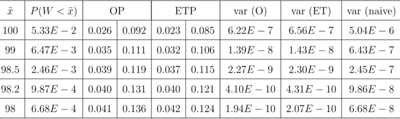
Table 3.12. Optimal and exponential twisting IS probabilities and correspond-ing variances to computeP(W <x˜). . . 48

Table 3.13. Optimal and exponential twisting IS probabilities and correspond-ing variances to computeE[W|W <x˜]. . . 49

Table 3.14. Variances for simulating P(L > x) under IS using optimal and exponential twisting probabilities and naive simulation. . . 51

Table 3.15. Variances for simulating E[L|L > x] under IS using optimal and exponential twisting probabilities and naive simulation. . . 51

Table 4.1. Tail loss probabilities and half lengths (hl) of the confidence in-tervals for naive, IS and the new method in the 10-factor model.

n= 10,000. Execution times (in seconds) are in parentheses. . . . 64

Table 4.2. ES values and half lengths (hl) of the confidence intervals using naive, IS and the new method in the 10-factor model. n= 100,000. Execution times (in seconds) are in parentheses. . . 64

Table 4.4. ES values and half lengths (hl) of the confidence intervals using naive, IS and the new method in the 21-factor model. n= 250,000. Execution times (in seconds) are in parentheses. . . 65

Table 4.5. Portfolio composition for the 5-factor model; default probabilities, exposure levels and factor loadings for six segments. . . 66

(17)

Table 4.7. ES values and half lengths (hl) of the confidence intervals using naive, IS and the new method in the 5-factor model. n = 100,000. Execution times (in seconds) are in parentheses. . . 66

Table 4.8. Tail loss probabilities and half lengths (hl) of the confidence inter-vals in a single simulation using naive, IS and the new method in the 10-factor model. n = 10,000. Execution times for the methods are 7, 16 and 12 seconds in the given order. . . 69

Table 4.9. ES values and half lengths (hl) of the confidence intervals in a single simulation using naive, IS and the new method in the 10-factor model. n= 100,000. Execution times for the methods are 66, 151 and 104 seconds in the given order. . . 69

Table 5.1. Half lengths (hl) of the confidence intervals for using tail bound ap-proximation (TBA), normal apap-proximation (NA) and homogenous approximation (HA) for the optimal mean shift as outer IS and ex-ponential twisting as inner IS in the 10-factor model to compute tail loss probabilities. n = 10,000. Execution times (in seconds) are in parentheses. . . 78

Table 5.2. Half lengths (hl) of the confidence intervals for using tail bound ap-proximation (TBA), normal apap-proximation (NA) and homogenous approximation (HA) for the optimal mean shift as outer IS and ex-ponential twisting as inner IS in the 10-factor model to compute expected shortfalls. n = 100,000. Execution times (in seconds) are in parentheses. . . 79

(18)

Table 5.4. Half lengths (hl) of the confidence intervals for using tail bound ap-proximation (TBA), normal apap-proximation (NA) and homogenous approximation (HA) for the optimal mean shift as outer IS and ex-ponential twisting as inner IS in the 21-factor model to compute expected shortfalls. n = 100,000. Execution times (in seconds) are in parentheses. . . 80

Table 5.6. Half lengths (hl) of the confidence intervals for using tail bound ap-proximation (TBA), normal apap-proximation (NA) and homogenous approximation (HA) for the optimal mean shift as outer IS and exponential twisting as inner IS in the 5-factor model to compute expected shortfalls. n = 100,000. Execution times (in seconds) are in parentheses. . . 81

Table 6.1. Achieved coverage levels for 95 percent upper and lower endpoint confidence intervals (x= 2) . . . 86

(19)

Table 6.2. Achieved coverage levels for 95 percent upper and lower endpoint confidence intervals (S0 = 100,r = 0.09). . . 87

Table 6.3. Nearly exact tail loss probabilities and upper and lower bound of the confidence intervals by using ordinary t statistics and Hall’s method in the 10-factor model. n= 1,000. . . 88

Table 6.4. Nearly exact tail loss probabilities and upper and lower bound of the confidence intervals by using ordinary t statistics and Hall’s method in the 21-factor model. n= 1,000. . . 89

Table 6.5. Nearly exact tail loss probabilities and upper and lower bound of the confidence intervals by using ordinary t statistics and Hall’s method in the 5-factor model. n = 1,000. . . 89

Table 6.6. Achieved coverage levels for 95 percent upper and lower endpoint confidence intervals for computing tail loss probabilities. n= 1,000. 90

Table A.1. Optimal and exponential twisting [13] probabilities and percent dif-ferences of variances between exponential twisting and optimal (% diff. of var. ET-O) and naive simulation and optimal (percent diff. of var. naive-O) forx= 1 in computing P(L > x). . . 94

Table A.2. Optimal and exponential twisting [13] probabilities and percent dif-ferences of variances between exponential twisting and optimal (% diff. of var. ET-O) and naive simulation and optimal (% diff. of var. naive-O) forx= 1 in computing E[L|L > x]. . . 95

Table A.3. Optimal and exponential twisting [13] probabilities and percent dif-ferences of variances between exponential twisting and optimal (% diff. of var. ET-O) and naive simulation and optimal (% diff. of var. naive-O) forx= 5 in computing P(L > x). . . 96

(20)

Table A.4. Optimal and Exponential Twisting ( [13]) probabilities and percent differences of variances between exponential twisting and optimal (% diff. of var. ET-O) and naive simulation and optimal (% diff. of var. naive-O) forx= 5 in computing E[L|L > x]. . . 97

(21)

LIST OF SYMBOLS/ABBREVIATIONS

ajl Factor loading of jth obligor for risk factorl A First group of obligors

B Second group of obligors

c Loss resulting from default of an obligor or homogenous loss

cA Loss resulting from default of an obligor in groupA cB Loss resulting from default of an obligor in groupB cj Loss resulting from default of jth obligor

c∞ 100(1−α)% quantile of L∞_d Cov(Zk, Zl) Covariance between Zk and Zl d Number of systematic risk factors

gj Weight for obligorj

E[T] Expectation of a random variable T

E[T|S] Expectation of a random variable T conditional on an event S

Eθ Expectation under exponential twisting with parameterθ

erf c(z) Complementary error function ofz

exp(z) Exponential function of z

I Identity matrix

L Total loss of portfolio

Li ith possible (having probability greater than zero) loss value in the portfolio loss distribution

L∞_d Infinite homogenous portfolio loss function

L(k) _{Total loss of portfolio for replication} _k

m Number of obligors in portfolio

mA Number of obligors in groupA mB Number of obligors in groupB

M2(x, θ) Second moment of estimator for P(L > x) for exponential twisting with parameter θ

(22)

nin Number of inner replications

Nµ,σ Normal density function with mean µand variance σ

p Default probability of an obligor or homogenous default prob-ability

P Probability measure

pA Default probability of an obligor in group A pB Default probability of an obligor in group B pj Marginal default probability ofjth obligor pnew IS default probability

pnew,A IS default probability for obligors in group A pnew,B IS default probability for obligors in group B P(S) Probability of an event S

¯

pZ Average of the conditional default probabilities for obligors Q Importance Sampling probability measure

rs Speed up ratio

s Scaling factor to normalize weighted sum of factor loadings

V ar[T] Variance of a random variable T

w Likelihood ratio

w(k) Likelihood ratio for replication k

X Multivariate normal vector of latent variables

Y Default indicator for an obligor (1 if default, 0 otherwise)

Yj Default indicator for jth obligor (1 if default, 0 otherwise) Z Multivariate standard normal random variable for systematic

risk factors

Zl Standard normal random variable for systematic risk factor l zδ/2 (1−δ/2) percentile of the standard normal distribution

1−α Probability level at which confidence interval is given

j Idiosyncratic risk factor for obligor j θ Exponential twisting parameter

µ Mean shift vector in IS

(23)

ψ Density function for Q

ψL(θ) Cumulant generating function of Lgiven θ

Φ Standard normal cumulative distribution function Ψ Weighted sum of factor loadings

CI Confidence Interval

ES Expected Shortfall

ET Exponential twisting

ETP Exponential twisting probability GSL GNU Scientific Library

HA Homogenous approximation hl Half length of confidence interval

IS Importance Sampling max Maximize NA Normal approximation O Optimal IS OP Optimal IS probability prob. Probability skw Skewness sd Standard deviation

sup Supremum (least upper bound) TBA Tail bound approximation

var Variance

VaR Value at Risk

VaRα Value at Risk at 100(1−α) percent confidence level

(24)

1. INTRODUCTION

Financial institutions are subject to a wide range of risks. [6] classifies them as market risk, credit risk, liquidity risk, operational risk and systematic risk. This thesis study considers only credit risk, which can be defined as risks associated with default of obligors to make payments or changes in their credit quality.

Measuring the credit portfolio risk is a challenge for financial institutions because of the regulations brought by Basel Committee [3]. In recent years lots of models (see [4]) and state-of-the-art methods, which utilize Monte Carlo simulation, (see [11]) were proposed to solve this problem. The proposed models are with the exception of CreditPortfolio View [27] factor based models. They use factors to account for the correlations in the defaults of obligors. This ease the calibration of the models and decrease computational effort for correlated losses. However, [20] report that multi-factor models should be adjusted to achieve Basel II-consistent results and they show how to do that.

We concentrate on the the normal copula model of [19], a Merton [29] type model, to capture the dependence across obligors. Underlying risk factors are assumed to be normal in this model. However, we are aware of the risks of using this model because of weak tail dependence (see [8]).

Value at Risk (VaR) has been quite popular as a risk measure to be used in credit risk models because of being conceptually simple and easy-to-compute. It is simply the quantile of portfolio loss distribution. [2] defines VaR at 100(1−α) percent confidence level (VaRα(X)) as

VaRα(X) = sup{x|P[X ≥x]> α}

(25)

Nevertheless, there are some shortcomings of VaR (see [1] and [2]). To summarize, it ignores losses beyond VaR and is not coherent. [1] proposes Expected Shortfall (ES) to solve the problems of VaR. ES is simply the expected amount of losses that are larger than the VaR level. Thus, ES is defined as:

ESα(X) =E[X|X ≥VaRα(X)]

for the 100(1−α) percent confidence level.

Computation of VaR and ES for realistic portfolio models is subtle, since, (i) there is dependency throughout the portfolio; (ii) an efficient method is required to compute tail loss probabilities and conditional expectations at multiple points simultaneously. This is why Monte Carlo simulation is a widely used tool here. But, simulation is not an easy option either. We need to apply variance reduction techniques such as IS, control variate, etc. (see [11], Chapter 4) for rare-event simulations, simulating tail loss probabilities and conditional expectations.

Variance reduction techniques for simulating tail loss probabilities and conditional expectations in the normal copula framework are “hot topics”. Previous studies in importance sampling (IS), in the the normal copula model, can be summarized as:

(a) outer IS: applying IS to common factors (see [7, 25]);

(b) inner IS: applying IS on the resulting conditional default probabilities (see [28]); (c) two-step IS: applying outer IS first, then inner IS (see [12, 13, 18]).

These papers apply different but similar methodologies to slightly different problems. Note that all these works were finished in the last 4 years.

[13] and [28] apply an importance sampling (IS) technique which utilizes expo-nentially twisted Bernoulli mass functions discussed in [31] for computing P(L > x). Furthermore, [18] applies IS approach of [13], to the integrated market and credit portfolio model described in [17].

(26)

[13] and [28] not only apply exponential twisting, but also show that it is “asymp-totically optimal”1 _{for loss exceedance probabilities. However, [15] shows that} asymp-totically optimality of IS based on exponential twisting is true only in one point. Moreover, [7] report that for practical purposes, asymptotically optimal IS methods may fail. Even, they may perform worse than naive simulation for a typical medium-sized portfolio. And, they propose an IS approach that is based on adaptive stochastic approximation of Robbins-Monro.

It is well known that whenever we have a large skewness in a simulation, standard method of usingtstatistc for the confidence interval construction for the mean does not give robust results (see [11]). However, there are studies on how to decrease the effect of skewness of the population when doing tests on the mean such as confidence interval construction and hypothesis testing. [23] propose a transformation (Johnson’s trans-formation) on the t variable to correct for the bias on the mean, but [21] reports that it fails to correct for skewness. [21] propose another transformation (Hall’s transforma-tion) that has desirable characteristics of monotonicity and invertibility to correct for both bias and skewness from the distribution oft statistic. Furthermore, [34] compares the performance of Johnson’s and Hall’s transformations and their bootstrap versions by looking at the coverage accuracy of one-sided confidence intervals.

The organization of the thesis is as follows.

In Chapter 2 we first describe the widely used dependency model across obligors in a credit portfolio called here the normal copula model (see Section 2.1). In that section we also introduce the notation, which will be used throughout the thesis. In Section 2.2 we talk about simulation and one of the classical variance reduction techniques, IS. Finally, we describe the IS approach of [13] for the normal copula model.

In Chapter 3 we show how to compute the optimal importance sampling proba-bilities for credit portfolios consisting of groups of independent obligors both for tail

1_{asymptotically optimality refers to the case where the second moment decreases at the fastest}

(27)

loss probability and expected shortfall simulation. In Section 3.1 we show that we can apply exponential twisting directly on the binomial distribution to simulate tail loss probabilities. In Section 3.2 we compare the optimal IS probabilities with the “asymptotically optimal” ones for groups of obligors. In Section 3.3 we show how our methodology which is used throughout the chapter can be used to compute optimal probabilities for two small financial examples.

In Chapter 4 we propose a new efficient simulation method for computing tail loss probabilities and conditional expectations in the normal copula framework. We replace inner IS by inner replications implemented by a geometric shortcut in the two-step IS of [13]. Section 4.1 analyzes the geometric shortcut for independent obligors. In section 4.2 we consider dependent obligors and introduce the geometric shortcut for inner replications. In Section 4.3 we add outer-IS to the inner replications of the geometric shortcut for a portfolio having dependent obligors. While Sections 4.1-4.3 concentrate on the efficient simulations for computing tail loss probabilities, Section 4.4 applies our new method to the simulation of conditional expectations. We summarize our numerical results in Section 4.5. Finally, we conclude in Section 4.6.

In Chapter 5 we evaluate outer IS strategies, which consider only shifting the mean of the systematic risk factors in the numerical examples of Chapter 4. In Section 5.1 we describe the tail bound approximation used in [13] and the normal approxi-mation used in Chapter 4, which are then used to find the mode of the zero-variance IS distribution. In Section 5.2 we describe the homogenous portfolio approximation of [25]. In Section 5.3 we assess the performance of these three ways to calculate the mean shifts for the numerical examples of Chapter 4.

In Chapter 6 we evaluate the performance of Hall’s transformation in correcting the confidence intervals for financial simulations that include IS. In Section 6.1 we give the details of Hall’s transformation. In Section 6.2.1 and 6.2.2 we describe a portfolio risk and an option pricing example and compare the coverage accuracy of one-sided confidence intervals using ordinary t statistic and Hall’s transformation. For both of the problems we have analytical solutions. In Section 6.3 we compare the performance

(28)

of Hall’s condence intervals and standard t intervals for the numerical examples of Chapter 4.

(29)

2. THE CREDIT RISK MODEL

2.1. The Normal Copula Model

We are interested in the the normal copula model of CreditMetrics (see [19]) for the dependence structure across obligors. We first of all give the notation used throughout the thesis which is similar to [13].

m: number of obligors in portfolio

Yj: default indicator forjth obligor (equal to 1 if default occurs, 0 otherwise) cj: loss resulting from the default of jth obligor

pj: marginal default probability of jth obligor

L=Pm

j=1cjYj: total loss of portfolio n: number of replications in a simulation

Our aim is to assess the distribution of tail loss probability and ES over a fixed horizon. Values of cj’s are known and constant over the fixed horizon. Furthermore, we assume that the marginal default probabilities (pj’s) are known.

The normal copula model introduces a multivariate normal vector (X1, ..., Xm) of latent variables to obtain dependence across obligors. Relationship between the default indicators and the latent variables are represented by

Yj =1{Xj>xj}, j = 1, ..., m,

whereXj has standard normal distribution and xj = Φ−1(1−pj), with Φ−1 inverse of the standard normal cumulative distribution function. Obviously, the threshold value of xj is chosen such that P(Yj = 1) =pj.

The correlations among Xj are modeled as

(30)

where j and Z1, ..., Zd are independent standard normal random variables with b2j +

a2

j1+...+a2jd = 1.While, (Z1, ..., Zd) are systematic risk factors affecting all of the oblig-ors, j is the idiosyncratic risk factor affecting only obligor j. Furthermore, aj1, ..., ajd are constant and nonnegative factor loadings, assumed to be known. Thus, given the vectorZ = (Z1, ..., Zd), we have the conditionally independent default probabilities

pj(Z) = P(Yj = 1|Z) = Φ ajZ+ Φ−1(pj) bj , j = 1, ..., m, (2.2) where aj = (aj1, ..., ajd). 2.2. Simulation

To evaluate the integrals Monte Carlo simulation is a widely used tool in many fields such as option pricing, risk management, communication engineering, etc.. Since, problems in risk management like in other fields can be written as an expectation under a probability measure, we could use Monte Carlo simulation to solve these problems. It has the advantage of giving an error bound on the final result but has the disadvantage of being rather slow compared to other numerical methods. Nevertheless, it is the fastest alternative for high dimensional integrals.

2.2.1. Naive Monte Carlo Simulation

If the integral we want to evaluate is

EP[g(x)] =

Z

g(x)φ(x)dx

where P is the probability measure with density function φ(x) then the above expec-tation is computed by 1 n n X k=1 g(x)

(31)

where x are random numbers generated from density φ(x) and n is the number of replications.

2.2.2. Importance Sampling

The confidence intervals produced by naive Monte Carlo simulations are too wide to give robust results for rare event simulations. This is why we need variance reduction methods such as Importance Sampling (IS), control variate, etc.. (see Chapter 4 of [11] for a good description of the methods and examples)

The fundamental idea of importance sampling is to modify the probability density in such a way as to reduce variance. If for a probability measure, P; we have density

φ; we can introduce a measure, Q; with new density, ψ; and rewrite the expectation via EP[g(x)] = Z g(x)φ(x)dx= Z g(x)φ(x) ψ(x)ψ(x)dx=EQ[g(x)w(x)]

where w(x) = φ_ψ(₍x_x)₎ is called likelihood ratio for IS weight. Our aim is to find a new density ψ such that g(x)w(x) under measure Q has a lower variance than g(x) under measureP. However, we shoud be careful about the distribution of the likelihood ratio (see [10] and [22]).

Since, we are concerned with default risks of obligors in credit risk, we want more defaults to occur in our IS simulation. Thus, we simply increase the default probabilities of obligors. But, the problem is how much to increase the default probabilities to obtain minimal variance.

In IS simulation, the above expectation is computed by

1 n n X k=1 g(x)w(x)

(32)

wherexare random numbers generated from densityψinstead ofφ. Thus, the variance of the new estimator is

1 n EQ[g(x) 2_w₍_x₎2_]₋₍_E P[g(x)])2 . (2.3)

However, the variance formula is as difficult as the original integral. So, for real world problems, the minimization is intractable. But, we can find optimal IS probabilities, minimizing (2.3) in special cases of credit risk problems (see Chapter 3) or we can apply the minimization on the upper bound of this equation in some cases (see below).

2.2.3. The Algorithm of Glasserman & Li

Here we describe the IS approach of Glasserman & Li [13] for simulating tail loss probability. [13] considers the simpler case of independent obligors before dependent obligors. In this case Y1, ..., Ym are independent Bernoulli random variables with pa-rameters p1, ..., pm. For the IS approach, they simply increase each default probability from pj to some larger value qj to make large losses more likely. Thus, the estimator

of P(L > x) is the product of the indicator 1{L>x} and the likelihood ratio

m Y j=1 pj qj Yj 1−pj 1−qj 1−Yj .

Exponential twisting suggest to use a one-parameter family of the form

pj(θ) =

pjeθcj

pjeθcj+ (1−pj)

(2.4)

for the IS probabilities. Here,θ is the exponential twisting parameter and if we choose

(33)

Under this condition, the likelihood ratio can be written as exp(−θL+ψL(θ)) where ψL(θ) = logE[exp(θL)] = m X j=1 log 1 +pj(ecjθ−1)

is the cumulant generating function ofL.

The next step is to optimize the parameter θ to minimize the variance of the simulation. To accomplish that it is enough to consider the second moment of the estimator, given by M2(x, θ) = Eθ e−2θL+2ψL(θ)₁ {L>x} ≤ exp(−2θx+ 2ψL(θ)) (2.5)

whereEθ is the expectation under exponential twisting distribution with parameterθ. Since, it is a difficult problem to optimize the second moment, [13] suggest to optimize the upper bound (2.5).

The minimizer θx is the unique solution to

ψ0_L(θx) =x (2.6)

for the case where E[L] = Pm

j=1pjcj < x and equal to 0 otherwise. Note that, a

standard property of exponential twisting is that the Eθ[L] = ψ

0

L(θx) when θx > 0 so that the expectation under the new measure is always greater than or equal to x. Algorithm given in Figure 2.1 shows the required steps of the method in more detail.

2.2.3.1. Two-step IS of Glasserman & Li: Dependent Obligors. In this secton, we con-sider the more interesting case where Yj’s are dependent. We consider dependence introduced through a normal copula. [13] applies “inner” IS as in the independent case, but they do so conditional on the common factorsZ = (Z1, ..., Zd)T.Conditional

(34)

1. Compute θ using (2.6) if E[L] =Pm

j=1pjcj < x otherwise setθ = 0.

2. Calculate pj(θ), j = 1, ..., m as in (2.4). 3. Repeat for replications k= 1, ..., n:

1. generate Yj, j = 1, ..., m, from pj(θ);

2. calculate total loss for replication k,L(k) ₌Pm

j=1cjYj;

3. calculate likelihood ratio for replication k, w(k) _{= exp(}_−θL(k)₊_ψ

L(θ)); 4. Return 1 n n P k=1 1_{_L(k)_>x_}w(k).

Figure 2.1. Tail loss probability computation using exponential twisting for independent obligors.

independent probabilities are given in (2.2).

It is possible to compute the conditional cumulant generating function from the conditional independent default probabilities as

ψL|Z(θ) = logE[exp(θL)|Z] = m

X

j=1

log(1 +pj(Z)(ecjθ−1))

and solve for the parameterθx(Z) that will minimize the upper bound of the second mo-ment of the estimator as in the independent case. That is, ifE[L|Z] =Pm

j=1pj(Z)cj < x then θx(Z) is the unique solution to

ψ_L0_|_Z(θx(Z)) =x. (2.7)

otherwise θx(Z) = 0.

[13] then define new conditional default probabilities

pj,θx(Z)(Z) =

pj(Z)eθx(Z)cj

pj(Z)eθx(Z)cj + (1−pj(Z))

, j = 1, ..., m. (2.8)

(35)

condi-tional independent default probabilities pj,θx(Z)(Z), j = 1, ..., m.

Since L is equal to the sum of the Yjcj’s,

e−θx(Z)L+ψL|Z(θx(Z))₁

{L>x} (2.9)

is the new IS estimator. Its conditional expectation isP(L > x|Z) and its unconditional expectation is therefore P(L > x).

[13] reports that for highly dependent obligors exponential twisting is not enough for reducing the variance because large losses occur primarily when we have large outcomes of Z. To further reduce the variance, they apply a second step of “outer” importance sampling to Z. For this they consider shifting the mean of Z from the origin to some point µ. See Chapter 5 for mean shift methods proposed in literature and their comparison. We call shifting the mean outer IS and twisting the conditional default probabilities inner IS. The likelihood ratio for the outer IS is

e−µTZ+12µ

T_µ

.

When multiplied by (2.9) this yields the two-step IS estimator

exp(−µT_Z₊ 1 2µ

T_µ₋_θ

x(Z)L+ψL|Z(θx(Z))1{L>x}

in which Z is sampled from N(0, µ) and then Yj’s are generated from the twisted conditional independent default probabilities pj,θx(Z)(Z), j = 1, ..., mto generate L.

What is left is to decide on the magnitude ofµ. [14] suggests choosingµby solving

µ= max z P(L > x|Z =z)e −1 2z T_z (2.10)

which is the mode of the zero-variance IS distribution for Z that would reduce variance in estimating the integral ofP(L > x|Z) with respect to the density of Z.

(36)

Solving for µ in (2.10) is not easy because we are indeed simulating to compute

P(L > x|Z = z). But, we can use some approximations for P(L > x|Z = z) to

compute µ(see Chapter 5). [13] uses a tail bound approximation in which

P(L > x|Z =z)≤e−θx(z)x+ψL|Z(θx(z))_.

They use this upper bound in (2.10) to solve for an approximate µ.

Algorithm given in Figure 2.2 shows the required steps of the method in more detail.

1. Compute µusing (2.10).

2. Repeat for replications k= 1, ..., n:

1. generate zl ∼N(µl,1), l = 1, ..., d, independently; 2. calculate pj(Z), j = 1, ..., m as in (2.2); 3. compute θx(Z) using (2.7) if E[L|Z] = Pm j=1pj(Z)cj < xotherwise set θ = 0; 4. calculate pj,θx(Z)(Z), j = 1, ..., m as in (2.8); 5. generate Yj, j = 1, ..., m, from pj,θx(Z)(Z); 6. calculate total loss for replication k,L(k) =Pm

j=1cjYj;

7. calculate likelihood ratio for replicationk,w(k)_{= exp(}_−µT_Z₊1 2µ T_µ−θ x(Z)L+ ψL|Z(θx(Z)); 3. Return _n1 n P k=1 1_{_L(k)_>x_}w(k).

Figure 2.2. Tail loss probability computation using two-step IS of [13] for dependent obligors.

[13] theoretically shows that exponential twisting for independent obligors and two-step IS for dependent obligors are “asymptotically optimal”. This means that the second moment of the IS estimator decreases at the fastest possible rate as the event we simulate becomes rarer.

(37)

3. OPTIMAL IS FOR INDEPENDENT OBLIGORS

In this chapter, we assume that obligors default independently. This indepen-dence assumption will allow the use use of the binomial distribution for the group of obligors having the same default probability under the simplification of cj = 1 for

j = 1, ..., m for simulating the loss probabilities and expected shortfalls.

3.1. Exponential Twisting for Binomial Distribution

We can use the binomial distribution to simulate for the P(L > x) given that obligors default independently,pj =p and cj = 1 for j = 1, ..., m. But the question is: Can we use exponential twisting directly on this binomial distribution?

Since, L=Pm

j=1cjYj =

Pm

j=1Yj, Lis a random variable with binomial distribu-tion. Thus P(L > x) = m X j=bxc+1 m j pj(1−p)m−j.

Applying exponential twisting as IS, the new probability of default becomes

pθ =

peθ

1 +p(eθ₋₁₎,

and the likelihood ratio is e(−θL+ψ(θ)) _where

ψ(θ) = m X j=1 log(1 +p(eθ−1)) = mlog(1 +p(eθ−1)) = log(1 +p(eθ−1))m.

(38)

So, the new estimator forP(L > x) is

1{L>x}e−θL+log(1+pθ(e θ₋₁₎₎m

= (1 +p(eθ−1))m1{L>x}e−θL.

If we take the expectation of the new estimator under the new measure;

Eθ[(1 +p(eθ−1))m1{L>x}e−θL] = (1 +p(eθ−1))me−θxEpθ[1{L>x}e −θ(L−x)_] = (1 +p(eθ−1))me−θxEpθ[1{L−x}e −θ(L−x)_] = (1 +p(eθ−1))me−θx m X j=bxc+1 m j pj_θ(1−pθ)m−je−θ(j−x) = m X j=bxc+1 m j pj_θ(1−pθ)m−je−θ(j−x)(1 +p(eθ−1))me−θx = m X j=bxc+1 m j pj_θ(1−pθ)m−je−θj(1 +p(eθ−1))m = m X j=bxc+1 m j peθ 1 +p(eθ₋₁₎ j 1− pe θ 1 +p(eθ₋₁₎ m−j e−θj(1 +p(eθ−1))m = m X j=bxc+1 m j pj (1 +p(eθ₋₁₎₎j 1 +p(eθ−1)−peθ 1 +p(eθ₋₁₎ m−j (1 +p(eθ−1))m = m X j=bxc+1 m j pj (1 +p(eθ₋₁₎₎j (1−p)m−j (1 +p(eθ₋₁₎₎m−j(1 +p(e θ₋ 1))m = m X j=bxc+1 m j pj(1−p)m−j 1 (1 +p(eθ₋₁₎₎m(1 +p(e θ₋ 1))m = m X j=bxc+1 m j pj(1−p)m−j.

It is nothing butP(L > x).So, the new estimator is an unbiased estimator ofP(L > x).

(39)

Table 3.1. Portfolio composition (one obligor case)

Exposure level (c) Default rate (p)

103 0.01

for P(L > x). The second moment of the new estimator is

M2(x, θ) = Eθ

e−2θL+2ψ(θ)1{L>x}

≤ exp(−2θx+ 2ψ(θ)).

To make the optimization problem simple, we minimize the upper bound. Thus,

ψ(θ)0 =x. (3.1)

The solution to (3.1) is θ = log(_px₍(1_m−₋p_x)₎). So, if E[L] = mp < x then θ = log(_px₍(1_m−₋p_x)₎) otherwise θ = 0.

3.2. Optimal IS Probabilities

We concentrate on a small number of groups of obligors to give optimal IS proba-bilities. But, this is not a weird assumption. For example, [17] make use of eight group of ratings in his model. We want to see the percentage difference of variances in using optimal and “asymptotically optimal” IS in this section.

3.2.1. One Obligor Case

We first of all consider the simplest case; there is only one obligor in our portfolio. Portfolio composition is given in Table 3.1. The loss distribution for this portfolio is given in Table 3.2. We should consider the case where 0< x < 103 so that P(L > x) is different than zero and 1.

(40)

Table 3.2. Loss Distribution for the portflio (one obligor case)

i Loss (Li) Probability of loss (P(Li))

1 103 0.01

2 0 0.99

3.2.1.1. Computing Tail Loss Probability. Our aim is to compute P(L > x). In this simplest case of a portfolio we have an analytical solution

P(L > x) =

2

X

i=1

1{Li>x}P(Li) = p

where Li is the loss distribution value which has probability greater than zero.

Naive and IS simulation algorithms are given in Figures 3.1 and 3.2. In the algorithm given in Figure 3.2, pnew is the IS default probability for the obligor.

1. Repeat for replications k= 1, ..., n: 1. generate Y from p;

2. calculate total loss for replication k,L(k) ₌_cY_; 2. Return _n1

n

P

k=1

1{L(k)_>x_}.

Figure 3.1. Naive simulation algorithm for P(L > x) (one obligor case)

1. Repeat for replications k= 1, ..., n: 1. generate Y from pnew;

2. calculate total loss for replication k,L(k) =cY; 3. calculate likelihood ratio for replication k, w(k) ₌ p

pnew; 2. Return _n1 n P k=1 1{L(k)_>x_}w(k).

(41)

We compute the expectations and variances of Naive and IS estimators;

E[Naive Sim. Estimator] = np

n =p

V ar[Naive Sim. Estimator] = np(1−p)

n2 =

p(1−p)

n E[IS Estimator] = npnew

p pnew n =p V ar[IS Estimator] = p pnew 2 npnew(1−pnew) n2 = p2 n 1−pnew pnew (3.2)

Our aim is to find the optimal value of pnew that will minimize the variance of the IS estimator. Thus, we take the derivative of 3.2 with respect to pnew

∂ ∂pnew p2 n 1−pnew pnew = p 2 n −pnew−(1−pnew) p2 new = 1 np 2 −1 p2 new <0.

So, optimal value of pnew is 1.

If we apply the IS methodology of [13] explained in section 2.2.3, the IS probability is equal to x_c if E[L] = pc < x otherwise equal to p. Thus, the IS probability given by (2.6) is quite different from the optimal one we have computed. And, indeed the optimal has a variance of zero.

3.2.1.2. Computing Conditional Expectation of Loss. Our aim is to computeE[L|L > x]. In this simplest case of a portfolio, we have an analytical solution of

E[L|L > x] = 1 P(L > x) 2 X i=1 Li1{Li>x}P(Li) =c

where Li are the loss distribution values having probabilities greater than zero.

(42)

1. Repeat for replications k= 1, ..., n: 1. generate Y from p;

2. calculate total loss for replication k,L(k) ₌_cY_; 2. Return Pn k=1L (k)₁ {L(k)_>x_} Pn k=11{L(k)_>x_} .

Figure 3.3. Naive simulation algorithm for E[L|L > x] (one obligor case)

1. Repeat for replications k= 1, ..., n: 1. generate Y from pnew;

2. calculate total loss for replication k,L(k) =cY; 3. calculate likelihood ratio for replication k, w(k) ₌ p

pnew; 2. Return Pn k=1L (k)_w(k)₁ {L(k)_>x_} Pn k=1w(k)1{L(k)_>x_} .

Figure 3.4. IS algorithm for E[L|L > x] (one obligor case)

We compute the expectations and variances of Naive and IS estimators;

E[Naive Sim. Estimate] = nc1p

nP(L > x) =

c1p

P(L > x)

V ar[Naive Sim. Estimate] = nc 2 1p(1−p) n2_P₍_{L > x}₎2 = c2 1p(1−p) nP(L > x)2

E[IS Estimate] = nc1pnew p pnew nP(L > x) = c1p P(L > x) V ar[IS Estimate] = pc1 pnew 2 npnew(1−pnew) n2_P₍_{L > x}₎2 = c2 1p2 nP(L > x)2 1−pnew pnew . (3.3)

Our aim is to find the optimal value of pnew that will minimize the variance of the IS estimator. Thus, we take the derivative of 3.3 with respect to pnew

∂ ∂pnew p2_c2 1 n 1−pnew pnew = p 2_c2 1 n −pnew−(1−pnew) p2 new = p 2_c2 1 n −1 p2 new <0.

(43)

Table 3.3. Portfolio composition (independent two obligors)

Exposure level (cj, j = 1,2) Default rate (pk, k =A, B)

Obligor A 103 0.01

Obligor B 105 0.05

Table 3.4. Loss Distribution for the portio (independent two obligors)

i Loss (Li) Probability (P(Li)) 1 c1+c2 = 208 0.01∗0.05 = 0.0005 2 c2 = 105 (1−0.01)∗0.05 = 0.0495 3 c1 = 103 0.01∗(1−0.05) = 0.0095 4 0 (1−0.01)∗(1−0.05) = 0.9405

[12] uses the same exponential twisting probabilities for expected shortfall con-tributions with tail loss probability computation. Thus, from the previous section we have seen that the exponential twisting probability is quite different from the optimal probability 1.

3.2.2. Two Obligors Case

In this section, we consider the two obligors case. They default independently. The portfolio composition is given in Table 3.3. The loss distribution for the portfolio is given in Table 3.4.

3.2.2.1. Computing Tail Loss Probability. Our aim is to compute P(L > x). It has the analytical solution

P(L > x) =

4

X

i=1

1{Li>x}P(Li)

(44)

Naive and IS simulation algorithms are given in Figures 3.5 and 3.6 to compute

P(L > x).

1. Repeat for replications k= 1, ..., n: 1. generate Y1 from pA and Y2 frompB;

2. calculate total loss for replication k,L(k) ₌_c

1Y1 +c2Y2; 2. Return _n1 n P k=1 1_{_L(k)_>x_}.

Figure 3.5. Naive simulation algorithm for P(L > x) (two independent obligors case)

1. generate Y1 from pnew,A and Y2 frompnew,B; 2. calculate total loss for replication k,L(k) ₌_c

1Y1 +c2Y2; 3. calculate likelihood ratio for replication k,

w(k)₌ pA pnew,A Y1 1−pA 1−pnew,A 1−Y1 pB pnew,B Y2 1−pB 1−pnew,B 1−Y2 ; 2. Return _n1 n P k=1 1_{_L(k)_>x_}w(k).

Figure 3.6. IS algorithm for P(L > x) (two independent obligors case)

If max{c1, c2}< x < c1+c2, the only possibility ofL > xis the case where two of

the obligors default at the same time. Since, the defaults are independent, the problem simplifies to the one company case where the default probability is the product of two default probabilities of the obligors. So, the multiplication of default probabilities in new measure should be equal to 1 for the optimal IS. Thus, pnew,A = pnew,B = 1 are the optimal values of the new default probabilities for this case.

If c1 ≤x≤c2;

E[Naive Sim. Estimator] = n[(1−pA)pB+pApB]

n =pB

V ar[Naive Sim. Estimator] = 1

n pB−p2B E[IS Estimator] = npnew,Apnew,B_ppA new,A pB

pnew,B + (1−pnew,A)pnew,B 1−pA 1−pnew,A pB pnew,B n =pB.

(45)

V ar[IS Estimator] = n n2 pnew,Apnew,B pA pnew,A pB pnew,B 2 + (1−pnew,A)pnew,B 1−pA 1−pnew,A pB pnew,B 2 −p2_B ! = 1 n p2_Ap2_B pnew,Apnew,B + (1−pA) 2 p2_B (1−pnew,A)pnew,B −p2_B ! = 1 n p2_Ap2_B(1−pnew,A) + (1−pA)2p2Bpnew,A pnew,Apnew,B(1−pnew,A)

−p2_B ! = p 2 B n p2 A(1−pnew,A) + (1−pA)2pnew,A pnew,Apnew,B(1−pnew,A)

−1 ! = p 2 B n p2

A−p2Apnew,A+pnew,A−2pApnew,A+p2Apnew,A pnew,Apnew,B(1−pnew,A)

−1 = p 2 B n p2_A+pnew,A−2pApnew,A pnew,Apnew,B(1−pnew,A)

−1

To minimize V ar[IS Estimator];

∂V ar[IS Estimator] ∂pnew,B = p 2 B n

−(p2_A+pnew,A−2pApnew,A)pnew,A(1−pnew,A) (pnew,Apnew,B(1−pnew,A))2

= p 2

B n

−(p2_A+pnew,A−2pApnew,A) pnew,Ap2new,B(1−pnew,A)

So, ∂V ar[IS Estimator]_∂p

new,B ≤ 0 if (p 2

A+pnew,A−2pApnew,A) ≥ 0 which necessitates pnew,A ≥ −p2

A

1−2pA for pA<0.5 andpnew,A ≤ −p2

A

1−2pA forpA >0.5.Since, these conditions are always satisfied, minimum is is attained for pnew,B = 1.

Then, if we put pnew,B = 1 into the equation and take the derivative with respect topnew,A;

(46)

∂V ar[IS Estimator] ∂pnew,A = p 2 B n 2pA−1 p2 new,A−pnew,A +pnew,A−2pnew,ApA+p 2 A p3 new,A−p2new,A + pnew,A−2pnew,ApA+p2A pnew,A−2p2new,A+p3new,A

! = 0. Solution is:    n pA,₂_ppA A−1 o if pA 6= 1₂ {pA} if pA = 1₂ .

To summarize, for all cases pA < 1₂, pA > 1₂ and pA = 1₂, the optimal solution is pnew,A=pA and pnew,B = 1.

Thus, the optimal solution is pnew,B = 1 and pnew,A = pA. This is nothing but the variance of the one company case where the default probability is equivalent topB.

Note that c2 ≤ x ≤ c1 is the same as the previous case but this time we should only change default probability of company A instead of B. So, the optimal solution ispnew,A = 1 and pnew,B =pB.

If x <min{c1, c2};

E[Naive Sim. Estimator] = n[1−(1−pA)(1−pB)]

n

=pA+pB−pApB =pe

V ar[Naive Sim. Estimator] = 1

n

e

(47)

E[IS Estimator] = n n " pnew,Apnew,B pA pnew,A pB pnew,B +(1−pnew,A)pnew,B 1−pA 1−pnew,A pB pnew,B +(1−pnew,B)pnew,A 1−pB 1−pnew,B pA pnew,A # = p_e V ar[IS Estimator] = n n2 " pnew,Apnew,B pA pnew,A pB pnew,B 2 +(1−pnew,A)pnew,B 1−pA 1−pnew,A pB pnew,B 2 +(1−pnew,B)pnew,A 1−pB 1−pnew,B pA pnew,A 2 −p_e2 # = 1 n " p2 Ap2B pnew,Apnew,B + (1−pA) 2 p2 B (1−pnew,A)pnew,B + (1−pB) 2 p2_A (1−pnew,B)pnew,A −p_e2 # . (3.4)

There is no easy analytical solution for pnew,A and pnew,B that minimizes (3.4). But, we can solve it numerically.

If we apply exponential twisting, the optimal solution for the default probabilities are pnew,A = pAe

θc1

1+pA(eθc1−1) and pnew,B =

pBeθc2

1+pB(eθc2−1) if x > pAc1 +pBc2 where θ is the

unique solution to (2.6) otherwise pnew,A=pA and pnew,B =pB.

Let’s see how exponential twisting perform with respect to the optimal proba-bilities in the numerical example of Table 3.3. We observe that exponential twisting probabilities are quite different than the optimal ones especially for large x values in Table 3.5. This makes great difference in standard deviations. Note that, results in this table are based on 1,000,000 number of replications for all of the methods.

(48)

Table 3.5. Optimal (OP) and exponential twisting probabilities (ETP) and corresponding standard deviations (sd) to computeP(L > x) (Two independent

obligors case).

x OP sd (O) ETP sd (ET) sd (naive)

pnew,A pnew,B pnew,A pnew,B

120 1 1 4.07∗10−18 0.377 0.773 7.80∗10−7 2.22∗10−5 110 1 1 4.08∗10−18 0.324 0.729 8.99∗10−7 2.22∗10−5 104 0.010 1 9.23∗10−16 0.295 0.701 4.96∗10−5 2.18∗10−4 100 0.250 0.750 4.76∗10−5 0.276 0.681 4.95∗10−5 2.37∗10−4 90 0.250 0.750 4.76∗10−5 ₀_.₂₃₃ ₀_.₆₂₉ ₅_.₀₉_∗₁₀−5 ₂_.₃₆_∗₁₀−4

3.2.2.2. Computing Conditional Expectation of Loss. Our aim is to computeE[L|L > x]. It has an analytical solution of

E[L|L > x] = 1 P(L > x) 4 X i=1 Li1{Li>x}P(Li)

where Li are the loss distribution values which have probabilities greater than zero.

E[L|L > x].

1. Repeat for replications k= 1, ..., n: 1. generate Y1 from pA and Y2 frompB;

2. calculate total loss for replication k,L(k) =c1Y1 +c2Y2; 2. Return

Pn

k=1L(k)1{L(k)_>x_}

Pn

k=11{L(k)_>x_}

Figure 3.7. Naive simulation algorithm for E[L|L > x] (two independent obligors case)

If max{c1, c2}< x < c1+c2, the only possibility ofL > xis the case where two of

(49)

1. generate Y1 from pnew,A and Y2 frompnew,B; 2. calculate total loss for replication k,L(k) ₌_c

1Y1 +c2Y2; 3. calculate w(k) = pA pnew,A Y1 1−pA 1−pnew,A 1−Y1 pB pnew,B Y2 1−pB 1−pnew,B 1−Y2 2. Return Pn k=1L (k)_w(k)₁ {L(k)_>x_} Pn k=1w(k)1{L(k)_>x_} .

Figure 3.8. IS algorithm for E[L|L > x] (two independent obligors case)

simplifies to the one company case where default probability is the multiplication of two default probabilities of the obligors. So, the multiplication of default probabilities in new measure should be equal to 1 for the optimal IS. Thus, pnew,A=pnew,B = 1 are the optimal values of new default probabilities for this case.

If c1 ≤x≤c2;

E[Naive Sim. Estimator] = c2(1−pA)pB+ (c1+c2)pApB

P(L > x) = c2pB+c1pApB P(L > x) E[IS Estimator] = 1 P(L > x) (c1+c2)pnew,Apnew,B pA pnew,A pB pnew,B +c2(1−pnew,A)pnew,B 1−pA 1−pnew,A pB pnew,B ! = c2pB+c1pApB P(L > x)

(50)

V ar[IS Estimator] = n P(L > x)2_n2 " (c1+c2)2pnew,Apnew,B pA pnew,A pB pnew,B 2 +c2₂(1−pnew,A)pnew,B 1−pA 1−pnew,A pB pnew,B 2 −(c2pB+c1pApB)2 # = 1 nP(L > x)2 " (c1+c2)2 p2_A pnew,A p2_B pnew,B +c2₂ (1−pA) 2 1−pnew,A p2_B pnew,B −(c2pB+c1pApB) 2 # . (3.5) If x <min{c1, c2};

E[Naive Sim. Estimator] = 1

P(L > x) " c1(1−pB)pA+c2(1−pA)pB+ (c1+c2)pApB # = c1pA+c2pB P(L > x) E[IS Estimator] = 1 P(L > x) " (c1+c2)pnew,Apnew,B pA pnew,A pB pnew,B +c2(1−pnew,A)pnew,B 1−pA 1−pnew,A pB pnew,B +c1(1−pnew,B)pnew,A 1−pB 1−pnew,B pA pnew,A # = c1pA+c2pB P(L > x)

(51)

Table 3.6. Optimal and exponential twisting probabilities and corresponding standard deviations (sd) to compute E[L|L > x] (Two independent obligors case).

x OP sd (O) ETP sd (ET) sd (naive)

pnew,A pnew,B pnew,A pnew,B

120 1 1 4.22∗10−12 ₀_.₃₇₇ ₀_.₇₇₃ ₀_.₃₂₄ ₉_.₃₀ 110 1 1 4.22∗10−12 0.324 0.729 0.374 9.30 104 0.020 1.000 2.90∗10−4 ₀_.₂₉₅ ₀_.₇₀₁ ₀_.₁₀₃ ₀_.₄₆₄ 100 0.248 0.753 0.082 0.276 0.681 0.086 0.422 90 0.248 0.753 0.082 0.233 0.629 0.089 0.421 V ar[IS Estimator] = n P(L > x)2_n2 " (c1+c2)2pnew,Apnew,B pA pnew,A pB pnew,B 2 +c2₂(1−pnew,A)pnew,B 1−pA 1−pnew,A pB pnew,B 2 +c2₁(1−pnew,B)pnew,A 1−pB 1−pnew,B pA pnew,A 2 −(c1pA+c2pB)2 # = 1 nP(L > x)2 " (c1+c2)2 p2 A pnew,A p2 B pnew,B +c2₂ (1−pA) 2 1−pnew,A p2 B pnew,B +c2₁ (1−pB) 2 1−pnew,B p2 A pnew,A −(c1pA+c2pB)2 # . (3.6)

We numerically solve (3.5) and (3.6) for the optimal probabilities. Table 3.6 presents how exponential twisting probabilities perform compared to the optimal prob-abilities when computing E[L|L > x] in the numerical example of Table 3.3. We ob-serve that exponential twisting probabilities are quite different than the optimal ones especially for largexvalues in Table 3.6. This makes great difference in standard devi-ations. Note that, results in this table are based on 1,000,000 number of replications for all of the methods.

(52)

3.2.3. One Homogeneous Group of Obligors

We show that we can use binomial distribution in IS of [13] to computeP(L > x) for an homogeneous portfolio in section 3.1. But, the question is what is the perfor-mance of using this approach to compute P(L > x) and E[L|L > x] compared to the optimal IS strategy.

Let’s take pj =p and cj = 1 from j = 1, ..., m so that L=Pm_j₌₁cjYj =Pm_j₌₁Yj is a random variable with binomial distribution with parameters p and m.

3.2.3.1. Computing Tail Loss Probability. Our aim is to computeP(L > x) which has an analytical solution of P(L > x) = m X i=bxc+1 m i pi(1−p)m−i

under the assumptions we make.

P(L > x).

1. generate L(k) from binomial distribution with parameters pand m; 2. Return _n1

n

P

k=1

1_{_L(k)_>x_}.

Figure 3.9. Naive simulation algorithm for P(L > x) (One homogeneous group of obligors case)

It is easy to show the unbiasedness of IS estimator. Our aim is to choose a pnew that will minimize the variance of the IS estimator.

(53)

1. generate L(k) from binomial distribution with parameters pnew and m; 2. calculate likelihood ratio for replication k, w(k) ₌ p

pnew L(k) 1−p 1−pnew m−L(k) ; 2. Return _n1 n P k=1 1_{_L(k)_>x_}w(k).

Figure 3.10. IS algorithm for P(L > x) (One homogeneous group of obligors case)

The variance of the IS estimator is

1 n " _m X i=bxc+1 p pnew 2i 1−p 1−pnew 2m−2i m i pi_new(1−pnew)m−i −   m X i=bxc+1 m i pi(1−p)m−i   2 # = 1 n   m X i=bxc+1 m i p2i₍₁₋_p₎2m−2i pi new(1−pnew)m −i −   m X i=bxc+1 m i pi(1−p)m−i   2 .

Since, the last term (square of the expectation of the naive and IS estimator) does not depend on pnew, it is enough to minimize the first term (second moment of the estimator). Thus, our optimization problem is

min pnew m X i=bxc+1 m i p2i₍₁₋_p₎2m−2i pi new(1−pnew)m −i

which we solve numerically.

Let’s see how exponential twisting probabilities perform compared to the optimal probabilities in a numerical example given in Table 3.7. We observe that exponential twisting probabilities are quite close to the optimal ones for x > 10. This is why we don’t see much difference in standard deviations. Note that, results in this table are based on 1,000,000 number of replications for all of the methods.

(54)

Table 3.7. Optimal and exponential twisting IS probabilities and corresponding standard deviations (sd) for the parameter values of m= 100 and p= 0.1 to compute

P(L > x).

x OP sd (O) ETP sd (ET) sd (naive) 30 0.311 1.51∗10−11 ₀_.₃₀₀ ₁_.₅₃_∗₁₀−11 ₇_.₇₈_∗₁₀−8 25 0.261 9.17∗10−9 0.250 9.35∗10−9 2.02∗10−6 20 0.212 1.54∗10−6 0.200 1.58∗10−6 2.84∗10−5 15 0.164 5.80∗10−5 0.150 6.15∗10−5 1.96∗10−4 10 0.122 3.57∗10−4 0.100 4.93∗10−4 4.93∗10−4

3.2.3.2. Computing Conditional Expectation of Loss. Our aim is to computeE[L|L > x] which has an analytical solution of

E[L|L > x] = 1 P(L > x) m X i=bxc+1 i m i pi(1−p)m−i.

Naive and IS simulation algorithms are given in Figures 3.11 and 3.12.

1. generate L(k) _{from binomial distribution with parameters} _p_and _m_; 2. Return Pn k=1L(k)1{L(k)_>x_} Pn k=11{L(k)_>x_} .

Figure 3.11. Naive simulation algorithm for E[L|L > x] (One homogeneous group of obligors case)

Under the assumption of large number of replications, the denominator of the ratio becomes P(L > x). So, it is easy to show the asymptotically unbiasedness of the IS estimator. Our aim is to choose a pnew that will minimize the variance of IS estimator.

(55)

1. generate L(k) from binomial distribution with parameters pnew and m; 2. calculate total loss for replication k,L(k) ₌_cY_;

3. calculate likelihood ratio for replication k, w(k) =

p pnew L(k) 1−p 1−pnew m−L(k) ; 2. Return Pn k=1L (k)_w(k)₁ {L(k)_>x_} Pn k=1w(k)1{L(k)_>x_} .

Figure 3.12. IS algorithm for E[L|L > x] (One homogeneous group of obligors case)

The asymptotic variance of the IS estimator is

1 nP(L > x)2 " _m X i=bxc+1 i2 p pnew 2i 1−p 1−pnew 2m−2i m i pi_new(1−pnew)m−i −   m X i=bxc+1 i m i pi(1−p)m−i   2 # = 1 nP(L > x)2   m X i=bxc+1 m i i2 p 2i₍₁₋_p₎2m−2i pi new(1−pnew) m−i −   m X i=bxc+1 m i ipi(1−p)m−i   2 .

Since, the last term (square of the expectation of the naive and IS estimator) does not depend onpnew, it is enough to solve forpnewthat will minimize the first term (second moment of the estimator) to minimize the variance. Thus, our optimization problem is min pnew m X i=bxc+1 m i i2 p 2i₍₁₋_p₎2m−2i pi new(1−pnew) m−i

which we solve numerically.

Let’s see how exponential twisting probabilities perform compared to the optimal probabilities in a numerical example given in Table 3.8. We observe that exponential twisting probabilities are quite close to the optimal ones for x > 10. This is why we don’t see much difference in standard deviations. Note that, results in this table are