Combinatorial optimization and metaheuristics

C

OMBINATORIAL

O

PTIMIZATION AND

M

ETAHEURISTICS

S. CONSOLI

SUPERVISOR: PROFESSOR K. DARBY-DOWMAN

ABSTRACT: Today, combinatorial optimization is one of the youngest and most active areas of discrete mathematics. It is a branch of optimization in applied mathematics and computer science, related to operational research, algorithm theory and computational complexity theory. It sits at the intersection of several fields, including artificial intelligence, mathematics and software engineering. Its increasing interest arises for the fact that a large number of scientific and industrial problems can be formulated as abstract combinatorial optimization problems, through graphs and/or (integer) linear programs. Some of these problems have polynomial-time (“efficient”) algorithms, while most of them are NP-hard, i.e. it is not proved that they can be solved in polynomial-time. Mainly, it means that it is not possible to guarantee that an exact solution to the problem can be found and one has to settle for an approximate solution with known performance guarantees. Indeed, the goal of approximate methods is to find “quickly” (reasonable run-times), with “high” probability, provable “good” solutions (low error from the real optimal solution). In the last 20 years, a new kind of algorithm commonly called metaheuristics have emerged in this class, which basically try to combine heuristics in high level frameworks aimed at efficiently and effectively exploring the search space. This report briefly outlines the components, concepts, advantages and disadvantages of different metaheuristic approaches from a conceptual point of view, in order to analyze their similarities and differences. The two very significant forces of intensification and diversification, that mainly determine the behavior of a metaheuristic, will be pointed out. The report concludes by exploring the importance of hybridization and integration methods.

1. INTRODUCTION

Combinatorial optimization (CO) is the general name given to the problem of finding the best solution out of a very large, but finite, number of possible solutions. It lies at the interface of Discrete Mathematics, Computer Science and Operational Research. Many real-life decision problems can be formulated as combinatorial optimization problems and consequently there is a large and growing interest in both theoretical and practical aspects of the subject. In practice, combinatorial optimization problems are often large-scale and difficult to solve. Thus, much attention has been given to studying computational complexity and algorithm design with a view to developing efficient

solution procedures. A combinatorial optimization problem P=

(

)

• A set of variables X =

{

}

• Variable domains D₁,...,D_n,

• Constraints among variables,

• An objective function f to minimize (maximize), where f :D₁×...×D_n →ℜ+. The set of all possible feasible solutions is

(

) (

)

{

}

{

}

S = = n n i∈ i

S is usually called a search (or solution) space, as each element of the set can be seen as a candidate solution. To solve a combinatorial optimization problem means to find a solution s*_{∈S with minimum (maximum) objective function value; that is, f (s*)≤f (s),}

∀s∈S. s* is called a “globally optimal solution” of (S, f) and let the set S*⊆S be the “set of globally optimal solutions”.

Examples of such problems are Network Flow Problems (e.g. Shortest Path Problem, Minimum Spanning Tree Problem, Maximum/Minimum Cost Flow Problem), Matching Problems (e.g. Cardinality Matching Problem, Job Assignment Problem, Maximum/Minimum Weight Matching Problem), Matroids (e.g. Maximization/Minimization Problem For Independent Systems, Matroid Intersection Problem, Matroid Partitioning Problem), Set Covering Problem, Colouring Problems (e.g. Vertex-Colouring Problem, Edge-Colouring Problem), 3-Occurrence Max-Sat Problem, Knapsack Problems, Bin-Packing Problem, Network Design Problems (e.g. Survivable Network Design Problem, Steiner Tree Problem), and Traveling Salesman Problem.

By considering the Knapsack Problem, it is easy to understand the difficulty of finding an optimized solution. Suppose a hitchhiker has to fill up his knapsack by selecting from among various possible objects those that will give him maximum comfort: these and many other example of Knapsack Problems can be mathematically formulated by numbering the objects from 1 to n, introducing a vector of binary variables xj (j=1,…,n)

having the following meaning:

⎩ ⎨ ⎧ = otherwise. 0 selected j object if 1 j x

Then, if pj is a measure of the comfort given by object j, wj its size and c the size of

the knapsack, the problem will be to select, from among all binary vectors x satisfying the constraint c x w n j j j ≤

∑

∑

There are many applications of the knapsack model. For example, suppose an investment of up to c dollars is to be made in one or more of n possible investments. Let pj

be the profit expected from investment j, and wj the required investment. It is self-evident

that the optimal solution of the knapsack problem above will indicate the best possible choice of investments.

A naive approach to solve the knapsack problem would be to examine all possible binary vectors x, selecting the best of those that satisfy the constraint. A full enumeration consists of 2n _{vectors and thus, for a computer with a clock frequency of 3.6 GHz (3.6 ⋅ 10}9

instructions per second, i.e. 1 instruction in 0.28 ⋅ 10-9 _{s), the time, t, to compute 2}n

instructions is given by:

(

)

For n = 60 vectors, for example, t≈ 10 years, and for n = 61 more than 20 years, almost 4 centuries for n = 65, and so on.

However, the (N.F.L.T.) No-Free-Lunch-Theorem (Martello and Toth, 1990) states that, if an algorithm performs well on a particular class of problems, having been designed to exploit the specific characteristics of the problem in question, then it necessarily pays for that with degraded performance on the other problems. The theorem is used as an argument against using generic searching algorithms (e.g. genetic algorithms and simulated annealing) without exploiting as much domain knowledge as possible. Alternatively, the theorem establishes that “a general-purpose universal optimization strategy is not possible, and the only way one strategy can outperform another is if it is specially adapted to the problem under consideration” (Ho and Pepyne, 2002).

So combinatorial optimization algorithms are custom-strategies; that is, they are optimization techniques specialized to the particular kind of problem being solved.

Complete (or exact) algorithms are guaranteed to find, for every instance of a specified CO problem of finite size, an optimal solution in bounded time (with proof of its optimality), while in approximate methods, the guarantee of finding an optimal solution is sacrificed for the sake of getting good solutions in a significantly reduced amount of time.

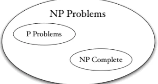
Combinatorial optimization problems can be classified as P-problems and NP-hard

problems. In computational complexity theory, the class P consists of all those decision problems that can be solved on a “deterministic sequential Turing-machine” in an amount of time that is polynomial p(x) in the size of the input x; the class NP consists of all those decision problems whose positive solutions⏐x⏐can be verified in polynomial-time p(⏐x⏐) given the right information, or equivalently, whose solution can be found in polynomial- time p on a “non-deterministic Turing-machine”. The term NP-hard (Non-deterministic Polynomial-time hard) refers to the class of problems that contains all problems H, such that for every decision problem L in NP there exists a “polynomial-time many-one reduction” to H, written L ∝H. Formally, H is NP-hard if

• There exists an L in NP and

FIG 1: Diagram of complexity classes provided that P ≠ NP. If P = NP, then all three classes are equal.

In computational complexity theory, a many-one reduction from L to H is a reduction that converts instances of the decision problem L into instances of the decision problem H. If there is an algorithm that solve instances of H, it is possible to use it to solve instances of L in:

− the time needed for N plus the time needed for the reduction;

− the maximum of the space needed for N plus the space needed for the reduction. Many-one reductions are a special case and a weaker form of Turing reductions; the latter are sometimes more convenient for designing reduction algorithms, but their power also causes several important classes, such as NP, to be not closed under this kind of reduction. Formally, a many-one reduction from L to H (or L many-one reducible to H) is a totally computable function , which is a function that can be calculated using a mechanical calculation device (i.e. it is possible to construct an algorithm that halts after a finite amount of time and decides whether or not a given element belongs or not to the function domain), such as

f f C D f : →

( )

Therefore, the “polynomial-time many-one reduction” from L to H is a many-one reduction which is computable by a deterministic Turing-machine in polynomial-time; while the term “C1 reducible to C2“ (written C1∝C2 ) means that for every instance a∝C1

there is a deterministic algorithm which transforms it into an instance b∝C2, such that the

answer of the “deterministic Turing-machine” to b is YES if and only if the answer to a is YES.

So, the notion of NP-hardness plays an important role in the discussion about the relationship between the complexity classes P and NP, because if it is possible to find an algorithm that solves one of these problems H in polynomial-time, it should be possible construct a polynomial-time algorithm for any problem L in NP by first performing the reduction from L to H and then running the polynomial algorithm. This would be equivalent stating “P = NP”, and thus solving the biggest open question in theoretical computer science concerning the relationship between these two classes. Indeed, a common mistake is to think that the word "NP" in "NP-hard" stands for "non-polynomial" but although it is widely suspected that there are no polynomial-time algorithms for these problems, this has never been proved.

Summarizing, if a NP-problem L is many-one reducible in polynomial-time to H, the

H is called NP-hard. This doesn’t mean that H is in NP: therefore, if it is also the case that

H is in NP, then H is called NP-complete (NP-C). FIG 1 shows the diagram of the complexity classes NP, P and NP-C, assuming that P ≠ NP. In a more formal way, a decision problem H is NP-complete if

• it is in NP and

• it is NP-hard (i.e. every other problem in NP is reducible to it).

A consequence of this definition is that if we had a polynomial-time algorithm for

H, we could solve all problems in NP in polynomial-time (“P = NP”). The NP-complete complexity class contains the most difficult problems in NP, in the sense that they are the ones most likely not to be in P. For more details see Garey and Johnson (1979) in which many NP-Complete problems are classified.

Numerous instances of problems arising in Operational Research and other fields are too large for an exact solution to be found in reasonable time. Thousands of problems are NP-hard and no algorithm with a number of steps polynomial in the size of the instances exists. Moreover, in some cases where a problem admits a polynomial algorithm, the power of this polynomial may be so large that realistic size instances cannot be solved in reasonable time in most of the cases (these are called long-term P problems). In this context (NP-C problems, long-term P problems, or in general problems difficult to solve), making use of exact algorithms is ineffective. So approximate algorithms should deal them in order to find “quickly” (reasonable run-times), with “high” probability, provable “good” solutions (low error from the real optimal solution). In the last 20 years, a new kind of approximate algorithms commonly called metaheuristics have emerged in this class, which basically try to combine heuristics in high level frameworks aimed at efficiently and effectively exploring the search space.

In the next section the basic concepts of metaheuristics will be outlined, allowing different kinds of classification between them.

In the sections 3 and 4, the most important single-point and population-based methods will be presented in order to analyze their similarities and differences, advantages and disadvantages and components from a conceptual point of view.

In the section 5, the two very significant forces of intensification and diversification, that mainly determine the behavior of metaheuristics, will be pointed out, concluding by exploring the importance of hybridization and integration methods in section 6.

2. CONCEPTSANDCLASSIFICATIONOFMETA-HEURISTICS

Approximate algorithms can be divided in two main classes: local-search algorithms and constructive algorithms. In short, the first class starts from an initial solution and it tries to replace the current solution at each step with a “better” one in a neighborhood of the current solution. Here the neighborhood of a current solution s is defined as a function , which assigns to every s ∈S a set of neighborhoods

N(s) ⊆S, where S is the search space. With the introduction of a neighborhood structure it is possible to define the concept of locally minimal solution (or local minimum) with respect to a neighborhood structure N(s), as a solution

( )

N : →2

The second class of approximate methods, constructive algorithms, builds a solution at each step, simply adding components to the solution of the previous step, until the constraints are satisfied. These methods are usually faster than local-search methods, but they also tend to be of lower quality.

In recent years, there have been significant advances in the theory and application of meta-heuristics to the approximate solution of hard optimization problems. The term

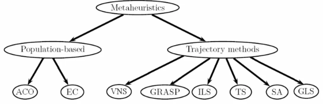
metaheuristic derives from the composition of two Greek words: “Heuristic” (from the verb heuriskein) that means “to find”; and the suffix “Meta”that means “beyond, in an upper level”. Before this term was largely adopted, metaheuristics were often called modern heuristics (Rayward-Smith V.J., Osman I.H., Reeves C.R. and Smith G.D, 1996). As illustrated in (FIG 2), this family includes, but it is not limited to, Tabu Search (TS), Simulated Annealing (SA), Explorative Local Search Methods including Greedy Randomized Adaptive Search Procedures (GRASP), Iterated Local Search (ILS), Variable Neighborhood Search (VNS) and Guided Local Search (GLS), Evolutionary Computation (EC) including Genetic Algorithms (GA) and Ant Colony Optimization (ACO).

As Voss S., Martello S., Osman I.H. and Roucairol C., (1999) state, “A metaheuristic is an iterative master process that guides and modifies the operations of subordinate heuristics to efficiently produce high-quality solutions. It may manipulate a complete (or incomplete) single solution or a collection of solutions at each iteration. The subordinate heuristics may be high (or low) level procedures, or a simple local search, or just a construction method”.

Summarizing, metaheuristics are strategies, approximate and usually non deterministic, that guide the search process to efficiently explore the search space in order to find (near-) optimal solutions, using techniques which range from simple local search procedures to complex learning processes. They are not problem-specific, can incorporate mechanisms to avoid “traps” (local optima), may use domain-specific knowledge to explore the best promising areas and finally they can memorize the search experience in order to guide the future search (long/short-time form of memory).

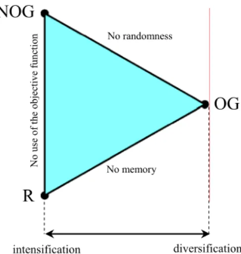
It is very important to clarify the concepts of diversification and intensification used in metaheuristics; the first term means the exploration of the search space while the latter one the exploitation of the accumulated search-experience. When the search process starts, it needs to compute the value of very different points in the search domain in order to find the promising areas (diversification). Then the algorithm needs to investigate promising zones to find the local-optimum (intensification). The best local optimum found in the different areas will be the candidate solution, hoping to be as near as possible to the optimum that the algorithm is looking for. The terms “diversification” and “intensification” are mainly used in methods based on the concept of memory, such as Tabu Search. Conversely the terms “exploration” and “exploitation” are used in strategies that don’t require explicit usage of memory, such as evolutionary computation. Finding a good balance between diversification (exploration) and intensification (exploitation) is essential for a metaheuristic in order to quickly identify regions in the search space with high quality solutions, without wasting too much time in regions with a low quality. Metaheuristics can be classified in different ways depending on the specific point of view of interest.

A first classification can be made by considering nature-inspired algorithms, such as Genetic Algorithms and Ant Algorithms, and non-nature inspired ones, such as Tabu Search and Iterated Local Search. This classification is not very meaningful because many

recent hybrid algorithms fit both classes at the same time and also because sometimes it is not possible to clearly attribute an algorithm to one of the two classes.

A second classification can be population-based, like Genetic Algorithms,and single point search methods, such as Tabu Search, Iterated Local Search and Simulated Annealing. The algorithms of this latter class are often called also trajectory methods because they work on a single solution at each time-step describing a curve (trajectory) in the search space during the progress of the search; they encompass local search-based metaheuristics. On the other hand, population-based metaheuristics compute simultaneously a set of points at each time-step of the search process, describing the evolution of an entire population in the search domain (FIG 2).

Metaheuristics can also be classified according to the way they make use of the objective function. If, during the search, the objective function is altered by trying to incorporate information collected during the search process (for example to escape from local minima), then the metaheuristic is said to have a dynamic objective function, as with the Guided Local Search (GLS). Techniques that keep the objective function as it is given by the problem belong to the class of metaheuristic with a static objective function.

Moreover, most metaheuristic algorithms work on one single neighborhood structure, i.e. the fitness landscape topology does not change in the course of the search process. Other metaheuristics, such as Variable Neighborhood Search (VNS), use a set of neighborhood structures (various neighborhood structures), diversifying the search by swapping between different fitness landscapes.

Finally, a very important feature to classify metaheuristics is the usage of a memory during the search history, because it is one of the fundamental elements of a powerful metaheuristic. In memory-less algorithms the next state depends only on the information accumulated in the current state of the search process, as a Markov process, while in

memory-usage algorithms there is a usage of a short-term and/or a long-term memory.

Usually, the first keeps track of recently visited solutions (moves), while the second is a huge storage of information about the entire search process.

The classification of metaheuristics in trajectory and population based methods permits a clear distinction between these kinds of algorithms. In the following sections, the most important single-point and population-based methods will be presented in order to analyze their similarities and differences, advantages and disadvantages and components from a conceptual point of view.

3. TRAJECTORYMETAHEURISTICS

Trajectory methods are so called because the search process designs a trajectory in the search space, starting from an initial state and dynamically adding a new better solution to the curve in each discrete time-step. So, this process can be seen as the evolution in time of a discrete dynamical system in the state space. The generated trajectory is useful because it provides information about the behavior of the algorithm and its dynamics in order to chose the most effective method to solve the problem instance under consideration. The system dynamics are the result of the combination of algorithms (i.e. chosen strategy), problem representation (i.e. definition of the search landscape) and problem instance. Trajectory shape depends on the strategy used: simple algorithms generate a trajectory composed of a transient phase followed by an attractor (a fixed point, a cycle or a complex attractor); advanced algorithms generate more complex trajectories comprising more different phases, representing the dynamic tuning between diversification and intensification during the search process. These continuous oscillations provide alternate phases in the designed trajectory, trying to find an optimal balance between these fundamental strengths. The main trajectory search methods are described below.

3.1 BASIC LOCAL SEARCH (OR ITERATIVE SEARCH)

Basic Local Search is the simplest trajectory search technique, and is often used in conjunction with other techniques. The concept is simple: every “move” from the current solution to the candidate solution is only performed if the objective function value given by the candidate solution is smaller than the value given by the current solution (in the case of a minimization problem). A move is the choice of a solution s’ from the neighborhood N(s)

of the previous solution s, that is s’∈N(s). The algorithm halts when a better solution can’t be found (i.e. the current solution is a local minimum). Formally, in pseudo code, the procedure may be specified as follows (Blum C. and Roli A., 2003):

s = Generate-Initial-Solution();

repeat

s = Improve(N(s));

until no improvements are possible

The procedure Improve(N(s)) can be in the extremes either a first improvement, or a

best improvement function, or any intermediate option. The former scans the neighborhood

N(s) and chooses the first solution that is better than s, the latter exhaustively explores the neighborhood and returns one of the solution with the lowest objective function value. Both methods stop at local minima. Therefore, their performance strongly depends on the definition of the search space S, of the objective function f andof neighborhood structure

N(⋅).

The effectiveness of a Basic Local Search tends to be highly unsatisfactory for combinatorial optimization problems, because it often becomes trapped in a local minimum. Some extra mechanisms have been developed to enable the procedure to escape from a local minimum, but they add computational complexity to the entire procedure.

Therefore, rather than as a stand-alone algorithm, Basic Local Search is usually used as a component in hybrid metaheuristics in order to improve performance to try solving a specific CO problem.

Possible termination conditions of a Basic Local Search could be:

− Reaching the maximum cpu time;

− Reaching the maximum total numbers of iterations;

− Finding a solution s with an objective function f(s) smaller than a threshold value;

− Achieving a maximum number of iterations without improvements.

3.2 SIMULATED ANNEALING (S.A.)

Simulated Annealing (SA) is possibly the oldest probabilistic metaheuristic for global optimization problems, and surely one of the first to explitly provide a way to escape from local traps. It was independently invented by Kirkpatrick S., Gelatt C. D. and Vecchi M. P. (1983), and by V. Cerny (1985). The SA metaheuristic performs a stochastic search of the neighborhood space. In the case of a minimization problem, modifications to the current solution that increase the value of the objective function are allowed in SA, in contrast to classical descent methods where only modifications that decrease the objective value are possible.

The name and inspiration of this method come from the process of annealing in metallurgy, a technique involving heating and controlled cooling of a material to increase the size of its crystals and reduce their defects. The heat causes the atoms to become unstuck from their initial positions (a local minimum of the internal energy) and wander randomly through states of higher energy; the slow cooling provides an opportunity to find configurations with lower internal energy than the initial one.

By analogy with this physical process, each step of the SA algorithm replaces the current solution by a random "nearby" solution, chosen with a probability that depends on the difference between the corresponding function values and on a global parameter T

(called temperature), that is gradually decreased during the process (cooling process). The dependency is such that the current solution changes arbitrarly in the search domain when T is large, i.e. at the beginning of the algorithm, through uphill moves (or

random walks) that saves the method from becoming stuck at a local minimum. Afterwards, the temperature T is gradually decreased, intensifying the search process in the specific promising-zone of the domain (downhill moves).

More precisely, the current solution is always replaced by a new one if this modification reduces the objective value, while a modification increasing the objective value by ∆ is only accepted with a probability e -∆/T_{. At a high temperature, the probability}

of accepting an increase to the objective value is high (uphill moves: high diversification and low intensification). Instead, this probability gets lower as the temperature is decreased (downhill moves: high intensification and low diversification).

The process described is memory-less because it follows a trajectory in the state space in which the successor state is chosen depending only on the incumbent one, without taking into account the past of the search process.

s = s0; //Generate-Initial-Solution() T = T0;

e = e0; //e0 > emax

k = 0;

while k < kmaxande > emaxdo

s’ = neighbor(s); //Pick-At-Random(N(s)) iff(s’) < f(s)then s = s’; //s’ replaces s else if rand() < ( ) ( ) T s f s' f − -e _then

s = s’; //Accepting a worse s’ as new solution with a given probability

endif endif

Update(T);

k = k + 1;

Endwhile //termination conditions met

returns;

The initial temperature value, the number of iterations to be performed, the temperature value at each step, the cooling (reduction) rate of T, and the stopping criterion are determined by the so-called “SA cooling schedule”, generally specified by the following rule:

Tk+1 = funct(Tk ,K);

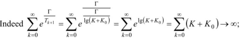
Theoretical results on non-homogeneous Markov chains (Aarts E. H. L., Korst J. H. M. and Laarhoven P. J. M. V., 1997) state that under particular conditions on the cooling schedule, the algorithm converges in probability to a global minimum for k→∞. More precisely, calling pk the probability to find a global minimum after k steps:

; 1 lim / 1 = ⇔ ∞ → ℜ ∈ Γ ∃ ∞ → ∞ = Γ

∑

So different cooling schedules, all satisfying this hypothesis of convergence, may be considered, such as a logarithmic cooling law:

(

)

( ) ( )

(

)

∑

∑

∑

∑

The drawback of this logarithmic cooling law is that it is too slow for practical purposes; therefore faster cooling schedule techniques are adopted in real applications, such as a geometric cooling law, which is a cooling rule with an exponential decay of the temperature:

[

0

,

1

]

where

;

=

⋅

∈

α

α

T

T

Other complex cooling techniques can be used in order to improve the performance of the SA algorithm. For example, to have an optimal balance between diversification and intensification, the cooling rule may be updated during the search process. At the beginning

T can be constant or linearly decreasing to have a high diversification factor for a larger exploration of the domain; after that, T can follow a fast rule, such as the geometric one, to converge quickly to a local optimum.

Other successful variants are non-monotonic cooling schedules that alternate phases of cooling and reheating, providing an oscillating balance between diversification and intensification.

Concluding, simulated annealing has been applied to several combinatorial problems, such as (Blum C. and Roli A., 2003):

− Quadratic Assignment Problem (QAP);

− Job Shop Scheduling (JSS) problem.

Rather than as a stand-alone algorithm, it is nowadays used as a component in hybrid metaheuristics to improve performance as in Threshold Accepting and Great Deluge Algorithms (Blum C. and Roli A., 2003).

3.3 TABU SEARCH (T.S.)

Tabu Search (TS) method, introduced by Glover (1986), is one of the most widely used metaheuristics. It shares with SA the ability to guide the search avoiding traps in poor local optima, but in a deterministic way rather than a stochastic one, modeling human memory processes.

Memory is implemented by the implicit recording of previously seen solutions using a simple data structure. This consists of a tabu list of moves which have been made in the recent past of the search, and which are forbidden (tabu) for a certain numbers of iterations. This helps to avoid cycling, and serves also to promote a diversified search of the solution, trying to escape from local minima.

At each iteration, TS moves to the best admissible neighbour restricted to the solutions that do not belong to the tabu list, referring to this set as the allowed set. The best solution from the allowed set is chosen as the new current solution, it is added to the tabu list and the oldest element of the tabu list removed (FIFO queue). Due to this dynamic

restriction of allowed solutions in a neighborhood, TS can be considered as a dynamic neighborhood search technique, with a short term memory implemented by the tabu list.

The entire algorithm stops when a termination condition is met or the allowed set is empty, as specified in the following procedure (Blum C. and Roli A., 2003):

s = Generate-Initial-Solution(); TabuList= ∅;

while termination conditions not met do s = Choose-Best-Of(N(s) \ TabuList); Update(TabuList);

Endwhile

Generally, usage of memory in metaheuristics can be described in terms of four “dimensions” in the search: recency, frequency, quality and influence, in which the first two are the most important.

Recency records the most recent iteration in which a solution was involved. In TS the most recent moves are forbidden and the length of the tabu list, called “tabu tenure”, represents the recency principle. The tabu tenure is either fixed or dynamically updated during the search process. If its value is small, there is a high exploitation of the domain, but not many uphill moves to differentiate the search. Otherwise, if the tabu tenure is large, the exploration of new areas is encouraged because it forbids revisiting a large number of solutions.

Obviously, it is more convenient varying the tabu tenure dynamically. For example, the tabu tenure could be periodically reinitialized at random between a minimum value and a maximum value. Otherwise, it could be manually increased if there are many solution repetitions (i.e. a larger diversification factor is needed), while it could be decreased if no improvements are obtained and more intensification is required.

It is often beneficial to focus on some components or attributes of a move rather than on the complete move itself, avoiding managing a list on entire solutions that could make TS inefficient and not practical. Attributes are stored in different tabu lists defining the tabu conditions, which are used to filter the neighborhood of a solution and generate the allowed set. A neighbouring solution is considered forbiddenand deemed not admissible if it has attributes on a tabu list.

Storing attributes rather than complete solutions is much more efficient, but also it may cause some non-tabu solutions, because forbidding an attribute means assigning the tabu status to probably more than one solution. To correct such errors aspiration criteria

are defined, enabling the introduction of a solution in the allowed set even if it is forbidden by tabu conditions. The most commonly used aspiration criterion selects elements that are better than the current solution.

If recency simulates the short-term memory, a long-term memory can be implemented by the use of a variety of frequency measures, as “residence” measures and “transition” measures. The former is related to the number of times a particular attribute is observed, while the latter relates to the number of times an attribute changes from one value to another. In each case, the frequency measures are usually employed to generate penalties, which modify the objective function. Thereby, diversification is encouraged by the generation of solutions embodying combinations of attributes significantly different

from those previously encountered. Conversely, intensification is promoted by incorporating attributes of solutions from selected subsets of elements, called elitesubsets, implicitly focussing the search in sub-regions defined relative to these subsets.

After discussing the concepts of recency and frequency, it may be also helpful to provide a brief reiteration of the basic notions of quality and influence.

Quality in TS usually refers to those solutions with good objective function values. A collection of such elite solutions may stimulate a more intensive search in the most promising regions of the search area.

Influence is roughly a measure of the degree of change induced in solution structure, commonly expressed in terms of the distance of a move from one solution to the next. It is an important aspect of the use of aspiration criteria, and is also relevant to the development of candidate list strategies. Influence is a property regarding choices made during the search and can be used to indicate which choices have shown to be the most critical.

The Tabu Search heuristic is a rich source of ideas. Many of these ideas together with the corresponding strategies have been, and are currently, adopted by other metaheuristics. From a practical point of view, a recency-based approach with a simple neighborhood structure, searched using a restricted candidate list strategy, will often provide very good results.

TS has been applied to most CO problems; examples of successful applications are (Blum C. and Roli A., 2003):

− Robust Tabu Search to the QAP;

− Reactive Tabu Search to the MAXSAT problem;

− multidimensional Knapsack problem;

− cutting and packing problems;

− assignment problems;

− Job Shop Scheduling (JSS) problems (TS dominates completely this area);

− vehicle routing.

3.4 EXPLORATIVE LOCAL SEARCH METHODS

Explorative Local Search Methods are a family of trajectory algorithms recently developed. The most important ones, such as GRASP (Greedy Randomized Adaptive Search Procedure), VNS (Variable Neighborhood Search), GLS (Guided Local Search), and ILS (Iterated Local Search), will be briefly explained below.

3.4.1 GRASP: GREEDY RANDOMIZED ADAPTIVE SEARCH PROCEDURE

GRASP is a recently exploited method combining the power of greedy heuristics, randomization, and local search. It mainly consists of a construction phase and a local search improvements phase, as specified in the following pseudo code procedure (Blum C. and Roli A., 2003):

GRASP ALGORITHM:

while termination conditions not met do

s = Construct-Greedy-Randomized-Solution(); // 1° phase

Apply-Local-Search(s); // 2° phase

Memorize-Best-Found-Solution();

Endwhile

1° phase – Construct Greedy Randomized Solution():

while termination conditions not met do

s = Construct-Greedy-Randomized-Solution(); Apply-Local-Search(s); // 2° phase

Memorize-Best-Found-Solution();

Endwhile

s = 0; // s denotes a partial solution in this case

α = Determine-Candidate-List-Length(); //def. of RCL length

while solution not complete do

RCLα = Generate-Restricted-Candidate-List(s); x = Select-Element-At-Random(RCLα); s = s ∪ {x};

Update-Greedy-Function(s); //update of the heuristic values

Endwhile

2° phase – Apply Local Search(s):

Solution-Improvement(); //e.g. S.A., T.S.

The solution construction mechanism is characterized by a dynamic constructive heuristic and by randomization: each solution is randomly produced step-by-step by uniformly adding one new element from a candidate list (RCLα) to the current solution.

RCLαis the restricted candidate list of length α that contains the best α elements of the

search space. The elements are ranked by means of a heuristic criterion that gives them a score as a function of the benefit if inserted in the current partial solution.

These values can be either static values (fixed from the starting point to the end of the entire algorithm) or dynamic values (updated at each step depending on the current partial solution). The length α of the restricted candidate list is a very important parameter because it determines the strength of the heuristic bias, and also influences the sampling of the search space. In the extreme cases:

• α = 1; only the best element would be added; construction mechanism is equivalent to a deterministic Greedy Heuristic;

• α = n; completely random construction mechanism; random-choice of elements from RCLα.

The simplest scheme to define α is updating it at each step, either randomly or by means an adaptive scheme.

After the solution construction phase, a local search is applied (such as S.A., T.S., iterative improvements) to try to improve the best current solution. The best element found

since the starting iteration is memorized, and the algorithm continues until the user termination conditions are reached.

Basic GRASP does not use history-memory of the search process and, for this reason, it is often outperformed by other metaheuristics. For its characteristics of simplicity and high speed, it is able to produce good solutions in a short amount of time. For example, it is a useful method for generating good starting points for other hybrid metaheuristics.

GRASP can be effective if the solution construction mechanism samples the most promising regions of the domain (by using an effective constructive heuristic and an appropriate value of α), and if the resulting solutions from the constructive heuristic belong to regions associated with different local minima (by using an effective constructive heuristic and an appropriate local search).

Successful applications of GRASP are (Blum C. and Roli A., 2003):

− Graph Planarization problems;

− grouping and clustering problems;

− production planning;

− vehicle routing;

− assignment problems;

− Job Shop Scheduling (JSS) problems.

3.4.2 VNS: VARIABLE NEIGHBORHOOD SEARCH

Variable Neighborhood Search is a new and widely applicable metaheuristic that makes use of a strategy based on dynamically changing neighborhood structures during the search process (Hansen and Mladenović, 1999, 2001, 2003, 2005). VNS provides a general framework and many variants exist for specific requirements. VNS doesn’t follow a trajectory, but it searches for new solutions in increasingly distant neighborhoods of the current solution, jumping only if they are better than the current best solution.

At the starting point it is required to define arbitrarily the neighborhood structure. The simplest and more ordinary choice is a structure in which the neighborhoods have increasingly cardinality: |N1(s)|< |N2(s)|< … < |Nmax(s)| (Nevertheless, with this sequence a

large number of solutions could be revisited, at the cost of increased computational time. Today, attempts to improve the scanning of the landscape are made through more complex neighborhood structures).

The process of changing neighborhoods in the case of no improvements corresponds to a diversification of the search. In particular the choice of neighborhoods of increasing cardinality yields a progressive diversification.

The VNS approach can be summarized in the sentence: “One Operator, One Landscape”, meaning that promising zones on the search space given by a specific neighborhood may not be promising for other neighborhoods (landscape). Nevertheless, a local optimum with respect to a given neighborhood may not be locally optimal with respect to another neighborhood.

VNS ALGORITHM:

Select a set of neighborhood structures Nk(s), with k =1… max;

// 0. Initialization phase, e.g. |N1(s)|< |N2(s)|< … < |Nmax(s)| s = Generate-Initial-Solution();

while termination conditions not met do k = 1;

while k < max do // Inner loop

s’ = Pick-At-Random (Nk(s)); // 1. Shaking phase ŝ = Local-Search (s’); // 2. Local search phase

if ( f (ŝ) < f (s)) then s = ŝ; // 3. Move phase k = 1; else k = k + 1; endif

Endwhile // end inner loop

Endwhile

The shaking phase consists of the random selection of a point s’ in the neighborhood of the current solution Nk(s). It provides a good starting point for the local search phase

because s’ may belong to a different basin of the current solution s (inner the Nk(s)), but

maintaining some good characteristics of it. The random point s’ is generated in order to avoid cycling, which might occur if any deterministic rule was used. The succeeding local search is not restricted to Nk(s) but any neighborhood structure can be used. Afterwards, if

no improvements are obtained (f (ŝ) > f (s)) in the move phase, the neighborhood structure is changed (k = k + 1) giving a progressive diversification (in the case of increasing cardinality neighborhoods |N1(s)| < |N2(s)| < … < |Nmax(s)|). As usual, the stopping

conditions may be to reach either the maximum allowed CPU time, the maximum number of iterations, or the maximum number of iterations between two succeeding improvements.

Numerous variants in VNS have been found. Experimentally, VNS performance can be improved if s’ is not just picked at random from Nk(s), but it is achieved by performing

an iterative search in the shaking phase between a random selection of points. Moreover, setting k = k + kstep instead of k = k + 1, and k = kmin instead of k = 1, gives an easy and

natural way to drive the intensification and diversification of the search. It is also possible to remove the local search step (RVNS: Reduced VNS) forvery large instances for which it is costly, making it similar to the classic Monte-Carlo method. Other more successful variants can be achieved and they will be described below.

A first important successful variant of VNS is the Variable Neighborhood Descent (VND) algorithm. It is based on the fundamental concept: the properties of a neighborhood are in general different from those of other neighborhoods and, therefore, a search strategy performs differently on them (Hansen and Mladenović, 2005). As Simulated Annealing, VND is a descent-ascent method because it may accept a worse candidate solution ŝ,

following a certain probability e-(f( ) ( )s' −f s) inserting in the move phase (Conversely, VNS is a descent method because it only accepts a candidate solution if it is better than the current one).

Moreover, instead of a first improvement strategy (used in the VNS shaking phase), VND makes use of a best improvement search in Nk(s) in order to improve its performance.

The VND algorithm can be obtained by substituting the inner loop of the VNS procedure, as specified in the following (Blum C. and Roli A., 2003):

VND ALGORITHM:

Select a set of neighborhood structures Nk(s), with k =1… max;

// 0. Initialization phase, e.g. |N1(s)|< |N2(s)|< … < |Nmax(s)| s = Generate-Initial-Solution();

while termination conditions not met do k = 1;

while k < max do // Inner loop

s’ = Chose-Best-Of (Nk(s)); if ( f (s’) < f (s)) then

s = s’; // Move phase

else

if rand() < e-(f( ) ( )s' −f s)then

s = s’; // Flexible move phase: Accepting a worse s’ as new solution with probability e-(f( ) ( )s' −f s)

else

k = k + 1; // no improvements: local minimum reached; let’s investigate in another neighbor

endif endif

Endwhile // end inner loop

Endwhile

The best improvementlocal search is applied in the current neighborhood (Chose-Best-Of (Nk(s))) and, in case a local minimum is found (i.e. no other improvements in that

neighbor), the search proceeds investigating if the solution found is also a local optimum for the successive neighborhood (k = k + 1). Conversely, if a move is performed (s = s’), the search will proceed with the same neighborhood structure until a minimum is reached. As in the classical VNS, the search will stop if either the maximum CPU time, the maximum number of iterations, or the maximum number of iterations between two improvements is reached. The choice of the neighborhood structures is the critical point in VNS and VND, because the neighborhoods should exploit different properties and characteristics of the search space. So another variant of VNS, called Variable Neighborhood Decomposition Search (VNDS), selects the neighborhoods producing a decomposition of the problem instance (Hansen and Mladenović, 2005). VNDS follows the usual VNS scheme, but the neighborhood structures and the local search are defined on sub-problems of each solution, All attributes (variables) of the current solution are kept fixed with the exception of k of them, which define a neighborhood structure Nk. Local search only regards changes on the

variables belonging to the sub-problem it is applied to.

VNDS procedure can be obtained by substituting the inner loop of the VNS algorithm, as specified in the following (Blum C. and Roli A., 2003):

VNDS ALGORITHM:

Select a set of neighborhood structures Nk(s), with k =1… max;

// 0. Initialization phase, e.g. |N1(s)|< |N2(s)|< … < |Nmax(s)| s = Generate-Initial-Solution();

while termination conditions not met do k = 1;

while k < max do // Inner loop

s’ = Pick-At-Random (Nk(s)); // 1. Shaking phase

ŝ = Local-Search (s’, k variables); // 2. Local search phase

if ( f (ŝ) < f (s)) then s = ŝ; // 3. Move phase k = 1; else k = k + 1; endif

Endwhile // end inner loop

Endwhile

In the shaking phase the current solution s and the incumbent one s’ differ only in k

attributes (variables); in the local search phase the new solutionŝis found by just allowing movements involving these k attributes. If a better solution ŝ is reached, the algorithm will start again setting k = 1 (i.e. the first neighborhood). Conversely, if no improving solutions are reached (f (ŝ) > f (s)) it means that the current solution s is a local minimum for k

variables; so the algorithm will increase the number of the variables (k = k + 1) and will go on the search. The algorithm will stop if the usual stop conditions are met.

VNS, VND, and VNDS are steepest descent-oriented algorithms and often they are unsuitable to effectively explore the search space. So another variant has been developed called Skewed VNS (SVNS), which extends VNS providing a more flexible acceptance criterion (Hansen and Mladenović, 2005). As an alternative to only accepting solution improvements, worse solutions s’’ can be accepted if they differ from the current one less than the value of α⋅ρ(s, s’’), where ρ(s, s’’) is the distance (previously defined) between s

and s’’, and αis a weight parameter in the acceptance criterion. The SVNS procedure is specified in the following pseudo code (Blum C. and Roli A., 2003):

SVNS ALGORITHM:

Select a set of neighborhood structures Nk(s), with k =1… max;

// 0. Initialization phase, e.g. |N1(s)|< |N2(s)|< … < |Nmax(s)| s = Generate-Initial-Solution();

while termination conditions not met do k = 1;

while k < max do // Inner loop

s’ = Pick-At-Random (Nk(s)); // 1. Shaking phase s’’ = Local-Search (s’); // 2. Local search phase

if ( f (s’’) - f (s) < α⋅ρ(s, s’’)) then // new accept. criterion

// solutions in the range α⋅ρ(s, s’’)

k = 1;

else k = k + 1;

endif

Endwhile // end inner loop

Endwhile

Variable Neighborhood Search and its variants have been successful applied to many CO problems (Hansen P. and Mladenović N., 2003), such as:

− Traveling Salesman Problem (TSP);

− vehicle routing;

− location and clustering problems;

− weighted MAXSAT problem:

− graph and network based problems;

− Job Shop Scheduling (JSS) problems.

3.4.3 GLS:GUIDED LOCAL SEARCH

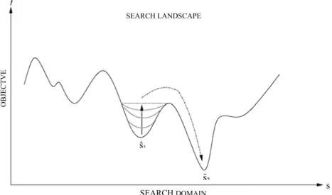
The Guided Local Search (GLS) approach gradually moves (to guide the search) away from local minima by changing the search landscape. In contrast to Tabu Search and VNS strategies, the set of solutions and the neighborhood structure are kept fixed while the objective function f is dynamically changed, in order to make the current local optimum less desirable and trying to escape from it (FIG 3).

f SEARCH LANDSCAPE ŝ1 ŝ2 s OB JE CT VE SEARCH DOMAIN

FIG 3: Guided Local Search strategy: escaping from traps increasing the relative objective function value, (Blum C. and Roli A., 2003).

This strategy is based on the definition of solution features, which may be any kind of properties or characteristics that can be used to discriminate between solutions (e.g. in TSP they could be arcs between pairs of cities, while in the MAXSAT problem the number of unsatisfied clauses could be considered).

An indicator function Ii(s) is defined to show if the feature i is present in a specific

solution s:

( )

The new objective function f’ is equal to the sum of the current objective function f

and a term depending on the m features:

( )

( )

∑

( )

where λ is the regulation parameter balancing the importance of features I respect the original f(s); pi are the penalty parameters weighting the importance of the specific

feature i. Before the actual search starts, the algorithm initializes all penalties parameters to zero, and assigns the variables uniformly at random. After each search phase, the penalties of all features with maximal utility are incremented by one, where the utility of a solution s

under feature i is defined as:

( )

( )

where ci is the cost assigned to feature i, obtained from an heuristic evaluation of the

relative importance of features with respect to others (the higher the costs, the higher are the utilities of the associated features). Nevertheless, the cost is scaled by the penalty parameter to prevent the algorithm from being totally biased toward the cost, making it sensitive to the search history. The GLS procedure is specified in the following pseudo code (Blum C. and Roli A., 2003):

s = Generate-Initial-Solution();

while termination conditions not met do for “all features I with Max Util(s, i)” do

pi = pi + 1; // or a variant is pi = α · pi with α∈ [0, 1]; end for

Update(f’, p);

Endwhile

where p = [p1, p2, …, pm] is the vector of penalties, updated in every search cycle,

together with the incumbent objective function f’.

A variant is to apply the penalties update rule (i.e. the multiplicative rule) with a lower frequency than with an incrementing rule (for example every few hundreds of

iterations), in order to smooth the weights of penalized features and to prevent the landscape from becoming too rugged. The penalty update rules are often very sensitive to the problem instance. Another extension of GLS uses an additional mechanism for bounding the range of the penalties: if after the updating process, the maximum penalty exceeds a given max threshold, all penalties are uniformly decayed, improving the performance of the algorithm and its efficacy to solve large and hard structured instances of problems.

Successful applications of GLS are (Blum C. and Roli A., 2003):

− Traveling Salesman Problem (TSP);

− vehicle routing;

− weighted MAXSAT problem;

− Quadratic Assignment Problem (QAP).

3.4.4 ILS: ITERATED LOCAL SEARCH

Iterated Local Search (ILS) mainly consists of two steps, the first to reach local optima performing a walk in the search space, while the second to efficiently escape from local optima. The aim of this strategy is to prevent getting stuck in local optima of the objective function. Iterated Local Search is probably the most general scheme among the explorative strategies. It is often used as framework for other metaheuristics or can be easily incorporated as subcomponents in some of them to build effective hybrids. Formally, in pseudo code its procedure may be specified as following (Blum C. and Roli A., 2003):

s0 = Generate-Initial-Solution();

ŝ = Local-Search(s0);

while termination conditions not met do s’ = Perturbation (ŝ, history);

ŝ’ = Local-Search (s’);

if ( f (ŝ’) <f (ŝ)) then // Move phase

ŝ= ŝ’; // improvements

else

ŝ = Apply-Acceptance-Criterion (ŝ, ŝ’, history); // acceptance // criterion for worse solutions

endif

Endwhile // end inner loop

The algorithm initializes the search by selecting an initial candidate solution s0. The

construction of s0 should be both computationally not expensive and a good starting point

for local search. The fastest way is to generate randomly the initial solution. However constructive heuristics may also be adopted in order to quickly find high-quality starting points. Afterwards, a locally optimal solution ŝ is achieved by applying a local search procedure, whose characteristics have a considerable influence on the performance of the entire algorithm.

1.A “perturbation” applied to the current candidate solution ŝ;

2.Another “local search” performed to the modified solution s’ in order to find a local optimum s’’;

3.The application of an “acceptance criterion” to decide which of the two local optima, ŝ’ or ŝ, has to be chosen to continue the search process.

The specific steps have to be properly designed and set to find a good tradeoff between intensification and diversification, and so achieving high performance in the difficult CO area. Both the perturbation and the acceptance criterion mechanisms can use aspects of the search history (long- or short-term memory). For example, stronger perturbation should be applied when the same local optima are repeatedly encountered.

The role of the perturbation (usually probabilistic to avoid cycling) is to modify the current candidate solution to help the search process to effectively escape from local minima, in order to eventually find different better points. Typically, the strength of perturbation has a strong influence on the length of the subsequent local search phase. It can be either fixed (independently of the problem size) or variable. However, the latter one is in general more effective because the bigger the problem size is, the larger should be the strength. A more sophisticated adaptive strength scheme is also possible in which the perturbation strength is increased when more diversification is needed, and decreased when intensification seems preferable (VNS and its variants belong to this category).

The acceptance criterion has also a strong influence on the behavior and performances of ILS. The two extremes are:

− Accepting the new local optimum only in case of improvement (strong intensification: iterative improvement mechanism);

− Always accepting the new solution (high diversification: random walk in the search space).

Between these extremes, there are several intermediate choices. It is possible, for example, to adopt a kind of annealing schedule: accepting all the improving candidate solutions and also the non-improving ones with a probability that is a function of the temperature T and the difference of objective function values (Blum C. and Roli A., 2003):

(

)

( ) ( )

-As in simulated annealing, the cooling schedule for the temperature T can be either monotonic (non-increasing in time) or non-monotonic (adapted to tune the balance between diversification and intensification). The non-monotonic schedule is particularly effective if it exploits the history of the search: instead of constantly decreasing the temperature, it is increased when more diversification seems to be required.

Successful applications of GLS are (Blum C. and Roli A., 2003):

− Traveling Salesman Problem (TSP);

− Single Machine Total Weighted Tardiness (SMTWT) problem;

4. POPULATION-BASED METAHEURISTICS

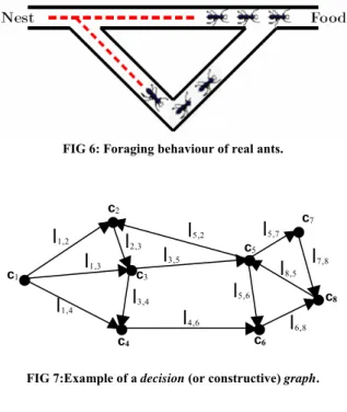
Population-based methods deal at each step with a set of solutions (or a population) rather than with a single one, providing a natural and intrinsic way to explore the search space. Their performance strongly depends on the way the populations are manipulated. The main population-based methods in combinatorial optimization are Evolutionary Computation (EC) and Ant Colony Optimization (ACO). In EC methods, specific recombination and mutation operators modify sets of individuals, while in ACO a colony of artificial ants is used to construct solutions guided by the pheromone trails and by heuristic information (as it will be specified in the following sections).

4.1 EVOLUTIONARY COMPUTATION

The field of natural evolution applied to optimization algorithms is at a stage of tremendous growth. The main idea consists of the survival of the best element in natural evolution processes. There are currently three well-defined paradigms, which have served as the basis for much of the research in this field:

− Genetic Algorithms (GA);

− Evolution Strategies (ES);

− Evolutionary Programming (EP).

Each of these emphasizes a different aspect of natural evolution. In general, they have foundation on the following evolutionary operators:

a) Recombination or crossover, which recombines two or more individuals (ancestors) to produce new individuals (children);

b) Mutation or modification, which causes a self-adaptation of individuals; c) Selection of individuals based on their fitness (value of an objective function or

some measure of the quality of solutions), which is the driving force in evolutionary algorithms. Individuals with a higher fitness have a higher probability to be chosen as members of the next population (or as parents for the generation of new individuals). This is an analogy with the principle of survival of the fittestin natural evolution, i.e. the capability of nature to adapt itself to a changing environment.

Formally, in pseudo code, the general EC procedure is specified as follow (Blum C. and Roli A., 2003):

P = Generate-Initial-Population (); Evaluate (P);

while termination conditions not met do P’ = Recombine (P);

P’’ = Mutate (P’);

Evaluate (P’’); P = Select (P ∪P’’);

EC methods often outperform classical optimization algorithms when applied to difficult real-world problems.

It is generally accepted that any EC algorithm must have five basic components (Michalewicz, 1996):

1) A genetic representation of problem solutions; 2) A way to create the initial population;

3) An evaluation function rating the solutions in terms of their fitness; 4) Genetic operators (already mentioned);

5) Values for the specific parameters (population size, probabilities of applying genetic operators, etc).

The data structure used to represent the solutions and the set of genetic operators, constitute the skeleton of each EC algorithm. Historically, there are associations between GA and binary string representations, between ES and vectors of real numbers (in order to perform numerical optimizations), and between EP and finite state machines (in order to build predictive systems). The EP and ES communities have emphasized a reproduction mechanism based on mutation. By contrast, the GA community emphasized reproduction based on recombination and mutation.

Genetic Algorithms have their origins from the studies of cellular automata conducted by John Holland (1975, 1992) and his colleagues, but only recently their potential for solving combinatorial optimization problems has been exploited. The term “Genetic Algorithms” is due to their genetic make-up representation and manipulation of individuals, rather than using a phenotypic representation. The basic idea is to maintain a population of candidate solutions, which evolves under a selective pressure helping the survival of the fittest individual. Hence, they are a class of local search methods employing solution generation, which operates on attributes of a set of solutions rather than attributes of a single solution. Genetic Algorithms work on finite populations each of which as N chromosomes (solutions). The chromosomes are fixed strings with binary values (alleles) at each position (locus). An allele is the 0 or 1 value in the bit string, while the "locus" is the position at which the 0 or 1 value is placed in the chromosome. Chromosomes are evaluated according to a specified fitness function, and are selectively interbred in pairs to produce offspring, through the genetic operators. The resulting offspring inherit properties directly from their parents. The fitter a chromosome is, the more likely it is to produce offspring. The offspring are evaluated and placed in the new population replacing the weaker members. The GA mechanism consists of three phases: evaluation of the fitness of each chromosome, selection of the parent chromosomes, and applications of mutation and recombination (crossover) operators to the parent chromosomes. The process is repeated until the system ceases to improve. The survival of the fittest ensures that the overall solution quality increases as the algorithm proceeds from one generation to the next one.

Differently from GA, Evolution Strategies were developed mainly to build systems capable of solving real-valued parameter optimization problems. Its natural representation of the individuals consists of a vector of real numbers in order to help mutation operators and gene manipulation. Generally, ES emphasize behavioral changes by mutation at the level of the individual.

The third EC approach is Evolutionary Programming, which stresses behavioral change at the level of the species. The phenotypes of individuals are represented as finite

state machines capable of reacting to environmental stimulation, and to develop operators (primarily mutation) for reflecting structural and behavioural change over time.

The Evolutionary Computation characteristics are summarized as follows (Blum C. and Roli A., 2003):

• DESCRIPTION OF INDIVIDUALS: EC deals with a population of individuals commonly represented as bit strings. In GA, the single individuals are called genotypes, while the solutions formed by combinations of individuals are called phenotypes;

• EVOLUTION PROCESS: In each evolution process, the selection operator is fundamental in choosing the individuals to enter the next population of each step. If they are chosen exclusively from the offspring, it is a case of a so-called “generational replacement” evolution process. Instead, if it is also allowed to transfer individuals of the current population into the next one, it is a case of a so-called “steady state” evolution process. Moreover, EC may work with a population of fixed or variable size;

• NEIGHBORHOOD STRUCTURE: EC can also deal with an unstructured population, in which any individual may be recombined with any other one to create an offspring (e.g. Basic GA). If any individual can be recombined with only those included in a particular set (e.g. Parallel GA), it is a case of a structured population;

• INFORMATION SOURCES: If the information sources for the crossover operations are just a couple of individuals, it is a case of a two-parents crossover scheme. Otherwise, if the offspring are produced by some recombination of more than two parents, it is the case of a multi-parent crossover. Recently clever crossover schemes were developed, such as Gene Pool Recombination (using population statistics to generate the individuals of the next population), or the Bit-Simulated Crossover (using a probability distribution over the search space given by the current population to generate the next one);

• INFEASIBILITY: there are three different ways to handle infeasible solutions generated by the genetic operators. Infeasible individuals could be simply “rejected”, “penalized” (by assigning them an additional bad fitness value, so that they will have difficulty in being reselected in the succeeding steps to create offspring), or just “repaired” (but it is not always possible);

• INTENSIFICATION STRATEGY: Some EC methods, including mechanisms to improve the exploitation of the fitness function, were designed in recent years. They have been shown to be useful in many practical applications. Memetic Algorithms, for example, apply a local search to every individual of a population to quickly identify promising areas in the search space (Moscato P., 1999). While the use of a population ensures the diversification of the search, the use of local search techniques improves the intensification factor on the promising zones. Another strategy performed by the so-called Linkage Learning and Building Block Learning algorithms, guides the search to promising areas, combining each parts of individuals with good properties (see (Goldberg D.E. at all, 1991), (Van Kemenade C. H. M., 1996), (Watson R.A. at all, 1998), (Harik G., 1999) as examples). Moreover, generalized recombination operators incorporating the notion of “neighborhood search” into EC, have been recently proposed in other novel methods (Rayward-Smith V. J., 1994);

• DIVERSIFICATION STRATEGY: A problem to avoid in EC algorithms is the premature convergence toward sub-optimal solutions. To try to avoid premature convergence, the simplest mechanism is the use of the mutation operator, which just

performs a small random perturbation on individuals (noise). Other strategies are the “crowding” mechanism, the novel “fitness sharing” and “niching”. They reduce the allocation of reproductive fitness to an individual in the population, proportionally to the number of other individuals sharing the same region in the search space.

Evolutionary Computation algorithms have been applied to most CO problems, such as (Blum C. and Roli A., 2003):

− multi-objective optimizati