Minimum Queue Length Load-Balancing in
Planned Wireless Mesh Networks
Germ´an Capdehourat, Federico Larroca and Pablo Belzarena
Instituto de Ingenier´ıa El´ectrica, Facultad de Ingenier´ıa, Universidad de la Rep´ublica, Uruguay {[email protected], [email protected], [email protected]}
Abstract—Wireless Mesh Networks (WMNS) have emerged in the last years as a cost-efficient alternative to traditional wired access networks. In order to fully exploit the intrinsically scarce resources WMNS possess, the use of dynamic routing has been proposed. We argue instead in favour of separating routing from forwarding (i.e. `a la MPLS) and implementing a dynamic load-balancing scheme that forwards incoming packets along several pre-established paths in order to minimize a certain congestion function. In this paper, we consider a particular but very important scenario: a planned WMN where all bidirectional point-to-point links do not interfere with each other. Due to its versatility and simplicity, we use the sum over all links of the mean queue length as congestion function. A method to learn this function from measurements is presented, whereas simulations illustrate the framework.
I. INTRODUCTION
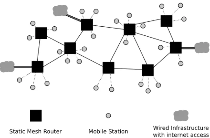
Wireless Mesh Networks (WMNS) [1] have emerged in the last years as a cost-efficient alternative to traditional wired access networks. In particular, outdoor community mesh networks [2] and rural deployments [3], [4] based on IEEE 802.11 have seen tremendous growth in the recent past. Under this scenario, the typical architecture (see Fig. 1) includes one or more gateways to the internet, and several relay routers.
The main challenge for this kind of networks, at the wireless mesh backbone level, is routing and forwarding. In the current standard [5] (and in several other proposals [6]) each link has an associated weight. This weight is expected to change over time, and reflect current conditions (propagation conditions, interference, etc.), so as to maximize a certain criteria (e.g. throughput). To choose a path to its destination, each router executes a shortest path algorithm. This procedure is essentially the same than the one used in wired networks. The main difference is that, just like in the internet until the early eighties, links weights are allowed to change at a time scale of some seconds [7]. The more static configuration that is used nowadays is due to the oscillations that these dynamic weights generated. It seems like history is repeating itself, since early experiments with WMNShave also reported routing oscillations [8], [9].
However, since resources are intrinsically scarce in WMNS, a static solution is not suitable. We argue instead in favour of a dynamic solution, but separating routing from forwarding. We propose a dynamic load-balancing scheme that forwards incoming packets along several pre-established paths in order to minimize a certain objective function. If correctly designed,
Static Mesh Router Mobile Station Wired Infrastructurewith internet access
Fig. 1. Wireless Mesh Network (WMN) typical architecture.
load-balancing will bring improved performance over static routing, without the difficult to avoid oscillations of pure dynamic routing (for more arguments in favour of load-balancing see the discussion presented in [10]). Due to its versatility and simplicity, we use the sum over all links of the mean queue length as objective function.
In this paper, we consider a particular but very important scenario: a planned WMN, where all bidirectional point-to-point links do not interfere with each other. This assumption means that either all backhaul links use different channels or links in the same channel are in different collision domains. There are many scenarios where this assumption holds, for example suburban or rural area networks and even campus networks, deployed with high directional antennas with proper RF design and channel assignment. This assumption also implies that the network topology is already defined (typically at infrastructure deployment phase), so we can not decide which backhaul links to establish but only how to use them (which traffic route through them). Unlike the wired case, the mean queue size at a given interface now depends not only on the incoming traffic, but also on the activity of the interface at the other end of the link.
There are some recent related works that we highlight. In [11] an optimization framework is presented to reach minimum average delay in a single channel WMN, while a load-aware routing metric was used in [12]. In [13] an heuristic algorithm was proposed to tackle the dynamic gateway
se-lection problem. A recent thesis [14] introduced a MPLS-based forwarding paradigm for WMNSusing a splitting-based routing policy.
Two major differences should be distinguished between our proposal and previous works. The first one is the introduction of a measurement-based model for 802.11 links, whereas most of the literature is based on (arbitrary) MAC layer models since Bianchi’s seminal paper [15]. The second important difference is the time scale at which decisions are taken. Most of routing algorithms proposed for WMNS are based on a certain metric which changes at a time scale of seconds. The presented framework operates at a flow level time scale, which enables decoupling the link model learning phase from the forwarding decision, and ensures better stability properties.
II. NETWORKMODEL ANDPROBLEMFORMULATION
Firstly, let us remark that in the context of WMNSwe may safely assume that nodes are fixed and do not change position very often and power is not an issue, so we will completely ignore energy consumption. We will then concentrate on the performance as perceived by packets in terms of delay, dropping probability and throughput. In this case, throughput will refer to a quantity proportional to the inverse of the time that it takes any given packet to leave the network.
Let n = 1, ..., N be the set of static wireless mesh
routers (including gateways) which we shall call nodes and
l = 1, ..., L the backbone bidirectional links in the network. Each node may have several wireless interfaces and we will assume that a single FIFO queue is attached to each interface (all packets are treated equally). We will focus on the mesh core, so only backhaul links and aggregated traffic at mesh routers will be considered. We will assume that this traffic uses different channels (e.g. 802.11a) than the ones used with mobile hosts (e.g. 802.11b/g). We shall further assume that channels within the mesh core do not interfere with each other. The traffic matrix is defined by a set of possible origin-destination (OD) pairs, which we shall index by the integer
s= 1, ..., S. The amount of traffic generated by OD pairswill be noted byds. As mentioned in Sec. I, each pair will have a
set ofnsfixed, establisheda prioripaths, which we shall note
as Ps. Each of the elements in Ps will be noted by Psi for
i= 1, ..., ns. The amount of traffic sent along pathPsishall be
noted asdPsi, which complies to the following two constraints:
P
idPsi = ds and dPsi ≥ 0. We further define the column
vectordas follows: d= [dP11...dP1n1dP21...dPS1...dPSnS]
T.
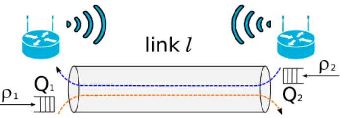
Within this context, for each linklwe have two traffic loads, one for each direction of the communication, which we shall callρl1 andρl2 taking any arbitrary convention (see Fig. 2). Given a demand vector d, the total traffic load on link l in one direction (e.g.ρl1) is given by the sum over all OD pairs of the demand of those paths dPsi which use the link in that
direction. Let Dl1 be the average amount of time a packet spends at the queue of linkl in the direction of loadρl1. This non-decreasing function depends on the loadρl1 and the load in the opposite direction ρl2, because of the 802.11 medium access control. Let DP be the average end-to-end delay of a
Q
1Q
2�
1�
2link
l
Fig. 2. Wireless link queues and flows in both directions.
path. Note that, as mentioned above, the throughput of pathP
is proportional to the inverse ofDP. We will use the mean total
delay D(d)as the total network congestion measure, defined as below. Then, it is easy to prove that:
D(d) := S X s=1 X P∈Ps dPDP = L X l=1 Dl1ρl1+Dl2ρl2 (1) Let Ql1 and Ql2 be the mean amount of bytes of link l queues on each direction. Then, by Little’s law we obtain the following result:Ql1 =Dl1×ρl1andQl2=Dl2×ρl2. Finally
D(d)is given by: D(d) = L X l=1 Ql1+Ql2= L X l=1 Ql(ρl1, ρl2) (2) In the next section we will present a measurement-based scheme to characterize Ql(ρl1, ρl2). As mentioned in Sec. I, we believe that the traffic distribution (i.e. the vectord) should be set so as to minimize the addition over all links ofQl. That
is to say, we should strive at solving the following problem:
min d L X l=1 Ql(ρl1, ρl2) s.t. dPsi ≥0 X dPsi = ds
We will now justify our choice of the objective function. Equation 1 suggests that our objective function may be re-garded as a weighted mean end-to-end delay, where the weight of each path is how much traffic is being sent along it. This means that P
lQl considers both delay and throughput at
the same time. Concerning dropping probability, the last of the three performance indicators cited before, it should be clear that a bigger value of it will result in a bigger queue at the output air interface, resulting in a bigger P
lQl. The
conclusion of this discussion is that P
lQl is a number that
is affected by the three performance indicators, and as such reflects the three of them. We referred to this when we said before thatP
lQl is a versatile indicator.
III. SIMULATION EXPERIMENTS
In order to test the proposed framework we performed several simulations with the ns-3 simulator [16]. Wireless links were set to 802.11a, all with a distance = 100m and fixed RSS = −65 dBm as propagation model. To generate each flow with the desired traffic load ρ, we used a combination of random TCP and UDP flows (80% and %20 respectively). TCP flows were generated with exponential file sizes with
0 5 10 15 20 0 5 10 15 20 0 4 8 −4 ρ2 (Mbps) ρ 1 (Mbps) log Q (pkts)
Fig. 3. Learnt function example (log-scale) for the link average queue length.
mean 500 Kbytes. UDP flows were generated with a fixed rate of 100 kbps and exponential length with mean 30 seconds. The arrival rate distribution was also exponential for both cases, with mean according with the desired traffic loads.
A. Wireless Link - Average Queue Length Function
The function Ql(ρl1, ρl2) is not trivial as we are dealing with wireless links with medium access control mechanisms like 802.11. Several works since [15] have tried to find the relation between wireless link parameters and the correspond-ing TCP and UDP achievable throughput. We used a different approach, that has already proved suitable for wired links [17], which is learning the function from measurements. The func-tion Ql(ρl1, ρl2) is assumed to be continuous, monotonous increasing and convex, which guarantees the existence and uniqueness of an optimum demand vectord, and it is approx-imated by a convex piecewise linear function. Differently to the wired case, the mean queue size at a given link is now a bi-variable function, because it depends not only on the incoming traffic, but also on the traffic in the opposite direction.
We present an example for one link to illustrate the pro-cedure followed for every link in the network in the learning phase. In the example we generated a dataset of 484 measure-ments, 228 used for learning the function and the remaining 256 for testing the regression performance. Each measurement corresponds to the average traffic load in both directions
(ρ1, ρ2)and the average queue lengthQl, where averages are
considered over 100 seconds. In Fig. 3 we present the resulting function after the regression in logarithmic scale. Queue size is expressed in packets because both ns-3 simulator and typical wireless equipment use 802.11 packet-based queues [18]. The RMSE for training data was 4.3 packets, while the RMSE for test data was 5.5 packets. The relative RMSE for training data was 2.9% with a maximum of 14.2%, while for test data was 4% with a maximum of 15.2%. This results show that the function approximation is suitable, which justifies the assumption of convexity. GW 0 GW 1
�
2�
01�
3�
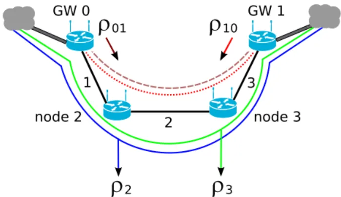
10 node 2 2 node 3 3 1Fig. 4. Network topology and traffic flows considered on simulations.
B. Optimization
In order to validate the framework we tested the proposed minimum queue length load-balancing (MQLLB) algorithm with simulations over the topology and flows shown in Fig. 4. We considered downlink flows to nodes 2 and 3 with traffic loadsρ2andρ3respectively. This traffic flows are distributed between the two gateways. We calledpGW0−2andpGW0−3the traffic portion ofρ2andρ3respectively, that is routed through gateway GW 0. Note that this gateway selection problem can be treated as a multipath forwarding problem. Both gateways could be considered as the same traffic origin (internet) and then the optimization problem to solve is exactly the same. We also considered the possibility to have inter-gateways flows, in this caseρ01 (from 0 to 1) andρ10 (from 1 to 0).
In order to drive the network to the desired operation point, we have to solve the optimization problem detailed in Sec. II. We used a gradient descent method to iteratively update the demand vector dby setting the proper load balance that leads to the optimum. Each iteration is performed every 100 seconds, the same time used for average measurements. The equation for updatingdat the stepn+ 1 is:
dnP+1 si = dnPsi−γ X l:l∈Psi ∂Ql ∂ρlsi ρnl1, ρnl2 +
where ρlsi is the traffic load of link l that corresponds to
path Psi. After updating d we have a normalization step to
guarantee the restrictions on the demands. Parameter γ was fixed in5×10−4 for all the experiments.
We used 200 measurements in the learning phase for each link, which is 5.56 hours of training data. We implemented the MQLLB method which uses the described optimization framework to iteratively update d, taking the forwarding decision with a flow level granularity.
In order to explain our algorithm operation we will analyze the case-scenario where traffic loads areρ01=ρ10= 3 Mbps andρ2=ρ3= 10 Mbps. The total queue evolution is shown in Fig. 5(a), where simulation starts at t = 0s with both flows routed through GW 0 (pGW0−2 = pGW0−3 = 1). At the beginning MQLLB is off which produces congestion at link 1, in the queue from GW 0 to node 2 (see Fig. 4). At
0 200 400 600 800 1000 1200 1400 1600 1800 2000 0 100 200 300 400 500 600 time (s) Q (pkts) Instantaneous Queue Average Queue
Theoretical Optimum Average Queue
(a) 0 200 400 600 800 1000 1200 1400 1600 1800 2000 0 50 100 150 200 250 300 350 400 time (s) Q (pkts) Total Queue Queue 0−>2 Queue 1−>3 (b)
Fig. 5. Optimization evolution for a simulation with traffic loadsρ01 =
ρ10= 3 Mbpsandρ2=ρ3= 10 Mbps.
time t = 1000s MQLLB starts running which produces an abrupt change in the total queue, which corresponds to the traffic portion which starts to be routed through GW 1. After two optimization steps (t = 1200s) we reached convergence to the optimum total queue. In Fig. 5(b) we can see the total queue evolution compared with the most important queues in this example, from GW 0 to node 2 and GW 1 to node 3.
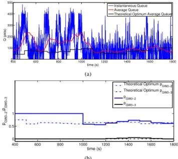
Now, we will take a look at another simulation example where traffic loads areρ01 =ρ10= 3 Mbps,ρ2 = 15 Mbps and ρ3 = 5 Mbps. In this case network started operating at
t= 0swithpGW0−2= 1andpGW0−3= 0, which corresponds to shortest path routing with hop count as routing metric. The heavy traffic load from GW 0 to node 2 produces congestion at link 1, which is visible in Fig. 6(a) where the total average queue evolution is shown from t = 400s, when we have already reached stationarity. MQLLB started operating at
t = 1000s and reached convergence at t = 1200s. The final total average queue length as we reached convergence is 79 packets, which is almost 50% smaller than before starting MQLLB where it was 154 packets (with peaks up to 235). The evolution ofpGW0−2andpGW0−3during the optimization is shown in Fig. 6(b).
C. Implementation Issues
The application of the proposed framework in a real-world network is relatively simple. First of all we need a routing protocol to establish the multiple routes for each OD pair defined by the wireless network topology. Once we have learnt Ql for every link l, each ingress router receives the
values ρl from the links used by the OD flows with origin
in that ingress router. A routing protocol that supports traffic engineering such as OSPF-TE may be used for this purpose. With that information, each ingress router is able to update the traffic portion that has to be routed through each path.
4000 600 800 1000 1200 1400 1600 1800 100 200 300 400 500 time (s) Q (pkts) Instantaneous Queue Average Queue
Theoretical Optimum Average Queue
(a) 400 600 800 1000 1200 1400 1600 1800 0 0.5 1 time (s) pGW0−2 ,pGW0−3 Theoretical Optimum p GW0−2 Theoretical Optimum p GW0−3 p GW0−2 p GW0−3 (b)
Fig. 6. Simulation under heavy traffic load conditions (ρ01 = ρ10 =
3 Mbps,ρ2= 15 Mbpsandρ3= 5 Mbps).
This process is repeated indefinitely every some seconds. This update period should be long enough so that the obtained measurements’ quality is reasonable, but not too long to avoid unresponsiveness (e.g. we used 100 seconds).
With respect to the flow-based multipath implementation, the idea is to use an MPLS-based solution, similar to the wired case. Although an standard of MPLS over WMNS
does not exist yet, several proposals were already presented. For example in [14] the proposal considers traffic splitting at every router and optimization over the average of all possible traffic matrices. Our proposal could be implemented reusing the same splitting-based scheme, but considering splitting only at ingress routers over all the different end-to-end paths and enabling dynamic load-balancing for the average load at each moment.
Regarding the learning phase we envisage several possibil-ities, differing in the resulting architecture distribution. One possibility is that a central entity gathers the measurements, performs the regression and communicates the obtained pa-rameters to all ingress routers. This option has the advantage that the required new functionalities on routers are minimal. However, as all centralized schemes, it may not be suitable for some network scenarios, and handling the failure of this central entity could be very complicated. An alternative is that for each wireless link only the two directly involved routers perform the regression. They should keep the average queue size measurements for themselves, perform the regression and communicate the result to the corresponding ingress routers.
Another aspect that has different possibilities is what char-acterization (i.e. Ql learnt function) use at each moment and
which measurements to keep for the training set. Measure-ments could be gathered every day, the regression performed, and its result could be used the next day or the same day the
next week. In addition, it is clear that newer measurements should be given priority over older ones. A possible way to manage training data is to keep always the newer measure-ments and use weights in the regression to introduce temporal information (e.g. exponential decay). It may also be necessary to force keeping particular measurements to ensure a proper coverage density of the whole range of possible load values.
For the gateway selection problem there is an important issue to solve for a real-world implementation. In this case we cannot perform path selection at the ingress routers because the gateway is usually defined by the routers which are directly connected to mobile hosts, which are egress routers for the dowlink traffic (typically the heavier load). One solution to this problem is to take the decision at these egress routers keeping a flow granularity, which implies to decide which gateway should be used for each client when a flow starts (e.g. joint with NAT). A simpler alternative is to make gateway selection with client granularity. In that case, these egress routers may decide the proper gateway for each client. In order to have a better resolution to define the amount of traffic coming from each gateway, these egress routers could monitor each client traffic demand. This way, the optimization process could use a client granularity but adding the client demand information, which allows a better traffic forwarding update at each step.
IV. CONCLUSIONS ANDFUTUREWORK
In this paper we proposed an algorithm for dynamic mul-tipath forwarding in a WMN. The algorithm enables load-balancing and conducts the network to operate at the minimum average congestion. The proposed framework also allows to solve the gateway selection problem in a WMN. This was achieved learning the average queue length function from measurements for each link and applying an optimization method in order to reach the minimum average queue length in the network. The proper evolution and convergence of the proposed method was verified by our packet-level simulations in a simple topology which serve as a proof of concept.
In our future work we will perform the learning phase with real data which includes among other issues the non-zero channel error rate, typical of a real-world wireless link. All the simulations presented in this paper are done with synthetic stationary traffic. We will extend our work to non-stationary real data which seems not to be a problem to the framework. It would be very interesting to perform a statistical analysis of the behaviour of the mean queue size with respect to the load. A possible analysis would be to study how often does the regression function change over time (i.e. answer the question of whether the mean queue size function changes over time, and how often it does). Another aspect of our future work is the implementation of the proposed framework in a real-world network which will serve as a testbed and could be used for enhancing the algorithm and detecting real-world driven problems that need to be solved. An interesting point which could be more profoundly studied in the future is the optimization phase. This problem could be solved by several different methods and was not analyzed in the present paper.
In particular, it could be worthwhile to study a parameter-free optimization method. Finally, we would like to extend the proposed framework, which was developed for a link disjoint WMN, to scenarios that have not only point to point links but also point to multipoint links.
ACKNOWLEDGMENTS
This work was partially supported by Centro Ceibal, CSIC (I+D project “Algoritmos de control de acceso al medio en redes inal´ambricas”) and ANII (grant POS 2011 1 3525).
REFERENCES
[1] I. F. Akyildiz, X. Wang, and W. Wang, “Wireless mesh networks: a survey,”Comput. Netw. ISDN Syst., vol. 47, pp. 445–487, March 2005.
[2] “Wireless community network list,” 2009. [Online]. Available:
http://www.toaster.net/wireless/community.html
[3] F. J. Sim´o Reigadas, P. Osuna Garc´ıa, D. Espinoza, L. Camacho, and R. Quispe, “Application of IEEE 802.11 technology for health isolated rural environments,” inWCIT 2006, Santiago de Chile, August 2006. [4] B. Raman and K. Chebrolu, “Experiences in using wifi for rural internet
in india,”IEEE Commun. Mag., vol. 45, no. 1, pp. 104 –110, Jan. 2007. [5] G. Hiertz, D. Denteneer, S. Max, R. Taori, J. Cardona, L. Berlemann, and
B. Walke, “IEEE 802.11s: The WLAN mesh standard,”IEEE Wireless
Commun., vol. 17, no. 1, pp. 104–111, Feb. 2010.
[6] R. Draves, J. Padhye, and B. Zill, “Comparison of routing metrics for static multi-hop wireless networks,” inACM SIGCOMM, 2004. [7] A. Khanna and J. Zinky, “The revised ARPANET routing metric,”
SIGCOMM Comput. Commun. Rev., vol. 19, pp. 45–56, August 1989. [8] K. Ramachandran, I. Sheriff, E. Belding, and K. Almeroth, “Routing
stability in static wireless mesh networks,” inPAM, 2007, pp. 73–83. [9] R. G. Garroppo, S. Giordano, D. Iacono, and L. Tavanti, “On the
development of a IEEE 802.11s mesh point prototype,” inTridentCom, 2008.
[10] M. Caesar, M. Casado, T. Koponen, J. Rexford, and S. Shenker,
“Dy-namic route recomputation considered harmful,”SIGCOMM Comput.
Commun. Rev., vol. 40, pp. 66–71, April 2010.
[11] J. Zhou and K. Mitchell, “A scalable delay based analytical framework
for CSMA/CA wireless mesh networks,”Comput. Netw., vol. 54, pp.
304–318, February 2010.
[12] E. Ancillotti, R. Bruno, M. Conti, and A. Pinizzotto, “Load-aware routing in mesh networks: Models, algorithms and experimentation,”
Comput Commun., vol. 34, no. 8, pp. 948 – 961, 2011.
[13] J. J. G´alvez, P. M. Ruiz, and A. F. G´omez-Skarmeta, “Responsive on-line gateway load-balancing for wireless mesh networks,”Ad Hoc Networks, vol. 10, no. 1, pp. 46–61, 2012.
[14] G. Di Stasi, “Design, analysis and evaluation of routing and channel assignment algorithms for wireless mesh networks,” Ph.D. dissertation, Universit`a degli Studi di Napoli Federico II, November 2011. [15] G. Bianchi, “Performance analysis of the IEEE 802.11 distributed
coordination function,” IEEE J. Sel. Areas Commun., vol. 18, no. 3, pp. 535–547, Mar. 2000.
[16] “The ns-3 Network Simulator.” [Online]. Available:
http://www.nsnam.org/releases/
[17] F. Larroca and J.-L. Rougier, “Minimum delay load-balancing via non-parametric regression and no-regret algorithms,”Computer Networks, vol. 56, no. 4, pp. 1152 – 1166, 2012.
[18] F. Li, M. Li, R. Lu, H. Wu, M. Claypool, and R. E. Kinicki, “Measuring queue capacities of ieee 802.11 wireless access points,” inBROADNETS, 2007, pp. 846–853.