Shuichi Katsumata Akiko Takeda The University of Tokyo
shuichi [email protected]
The University of Tokyo [email protected]
Abstract
In this paper we consider robust classifica-tions and show equivalence between the regu-larized classifications. In general, robust clas-sifications are used to create a classifier ro-bust to data by taking into account the un-certainty of the data. Our result shows that regularized classifications inherit robustness and provide reason on why some regularized classifications tend to be robust against data. Although most robust classification problems assume that every uncertain data lie within an identical bounded set, this paper consid-ers a generalized model where the sizes of the bounded sets are different for each data. These models can be transformed into regu-larized classification models where the penal-ties for each data are assigned according to their losses. We see that considering such models opens up for new applications. For an example, we show that this robust clas-sification technique can be used for Imbal-anced Data Learning. We conducted experi-mentation with actual data and compared it with other IDL algorithms such as Cost Sen-sitive SVMs. This is a novel usage for the robust classification scheme and encourages it to be a suitable candidate for imbalanced data learning.
1
Introduction
Many data provided in real-life problems are not given precisely, but instead, corrupted with some kind of er-ror or measurement noise. In such cases, it is common for the uncertainty of the data to be characterized by Appearing in Proceedings of the 18th International Con-ference on Artificial Intelligence and Statistics (AISTATS) 2015, San Diego, CA, USA. JMLR: W&CP volume 38. Copyright 2015 by the authors.
some bounded set which we call the uncertainty set. Robust optimization [5] is an approach that can handle optimization problems with prior bounds on the size of the uncertainties of the data. Solutions obtained from the robust optimization approach are more sta-ble for this kind of uncertainty. Intuitively, robust op-timization takes in account for all the points within the uncertainty set and solves for the worst possible case, thus creating a solution robust to the uncertainty of the data.
In the field of machine learning, data corrupted with uncertainties have been dealt with very often. In recent years, many active research on incorporating these uncertainties into formulation of the model has been made [23, 11, 18, 13]. Among them, the field of classification, the support vector machines (SVMs) in particular, has adapted very well with the robust optimization techniques.
SVMs [10, 8] have been studied in great depth and is known to be one of the most successful algorithms for classification. However, often time the data used for SVM are corrupted by some noise and it is necessary to incorporate these uncertainties into the model for-mulation. Many researches has been made on how to incorporate this prior knowledge into the SVM model. Usually, some sort of uncertainty sets are assigned to each data and a robust optimization problem is for-mulated. For an example, Trafalis and Alwazzi [19], Trafalis and Gilbert [20], Shivaswamy et al. [18], Bhat-tacharyya et al. [7] considered uncertainty sets for each data and allowed them to move within the uncertainty sets individually. Intuitively, this allows the data to si-multaneously take the worst case. On the other hand, Xu et al. [24] assigned uncertainty sets for each data, but also considered the data to have correlated noises. In other words, they restricted the aggregated behav-ior of the data uncertainty and limited them to not simultaneously take the worst case, making the solu-tion less conservative than prior methods.
However, most research on robust SVM focuses pri-marily on the formalization of the model, and to pro-vide numerical results on the stability of the
classi-fier. Owing to this, although connections between the robust and regularized classifiers has been known to some extent [11, 2], not many works concentrating on the explicit relationship between them have been made. We also point out that, to the best of our knowl-edge, in previous robust SVM models every data were assumed to lie within an identical uncertainty set. Al-though this is suitable for cases where each data are equally corrupted with the same type of noises, it does not fully capture real-life situations where the credibil-ity of each data might differ, e.g., as when the data rep-resent some particular person’s blood pressure, blood-sugar level and so on.
In this paper, our main objective is to show the ex-plicit equivalence between the robust SVM and the non-robust regularized SVM. For the robust SVM, we consider a generalized setting of previous models, where different sizes of uncertainty sets are assigned to each data. The equivalence provides reason to why regularized classifiers tend to be robust against data and explicitly shows that the norm-based regulariza-tion terms are created generically from the uncertainty sets assigned to the data. For an example, we see the standard robust SVM is equivalent to a non-regularized robust SVM with spherical (L2-norm) un-certainty sets on the data. This allows for an alter-native explanation on the properties of different types of regularized SVMs and provides for a richer under-standing. Furthermore, although the regularizer for the non-robust regularized SVM are usually chosen by the user’s preference, these observations also provide an alternative method on constructing the regularizer that might be more applicable to the problem. For instance, if the features of the data are independent we can assume a box-type (L∞-norm) uncertainty set around the data, which in return is equivalent to solv-ing a L1-norm regularized SVM.
We also observe that considering a generalized robust classification framework as above allows for novel ap-plications. In particular, we propose a cost sensitive learning paradigm for learning imbalanced data sets. Usually in cost sensitive SVM [15, 3, 21], the class with less data (the minority class) are assigned with higher costs than the class with more data (the major-ity class). This approach allows to bias the classifier so that it pays more attention to the minority class. In contrast, in our robust SVM model we assign larger un-certainty sets on the minority class and assign smaller uncertainty sets on the majority class. This is equiva-lent to a regularized SVM where the costs are assigned respective to the dual variables ζ, which denotes the amount of misclassification error of a particular data. This presents that robust SVMs can be formulated for cost sensitive classifiers as well. We evaluate the
ro-bust SVM model against imbalanced datasets and see that it has an effect of oversampling the minority data. We provide computational results to confirm that the proposed robust SVM model is suitable for imbalanced data learning.
1.1 Outline of the paper
In Section 2, we provide basic background information on robust optimization. Then we show our main re-sult, the explicit equivalence between the robust SVM and the regularized SVM. In Section 3, we look at spe-cific regularized SVMs, i.e., the standard non-robust SVM and the elastic net SVM, and provide alterna-tive explanations on the properties of each classifier from a robust classification perspective. In Section 4, we propose a new robust SVM model for imbalanced data learning and provide computational results. Fi-nally, in Section 5, we conclude the paper and look at some open questions.
1.2 Notation
Capital letters are used to denote matrices, boldface letters are used to denote column vectors. For a given matrix A and a vector x, AT and xT denotes their transpose respectively. k · kq denotes theq-norm.
Fi-nally, for a given two setsS andT, we defineS+T as the set {s+t|s∈S, t∈T}.
2
Robust Classification and
Regularization
2.1 Robust Classification
We consider a binary classification problem, where we try to find the best linear hyperplane that separates the data {(xi, yi)}mi=1. The vector xi ∈ Rn denotes the data and the scalar yi∈ {−1,1} denotes the class
data xi belongs to. This problem is solved through
the following optimization problem. min w,b,ζ r(w) +C Pm i=1ζi s.t. yi(wTxi+b)≥1−ζi, ζi≥0 i= 1,· · · , m, (1)
wherer(w) is the regularizer andCis a positive hyper-parameter. By substitutingr(w) =1
2kwk 2
2, we obtain the standard soft marginC-SVM.
However, in real life situations, the data are rarely given precisely due to modeling errors and measure-ment noises, and some kind of perturbation is accom-panied with. Therefore, taking uncertainty and am-biguity of data into consideration when formulating an optimization problem is of significant practical im-portance [5]. Robust optimization is one of the basic
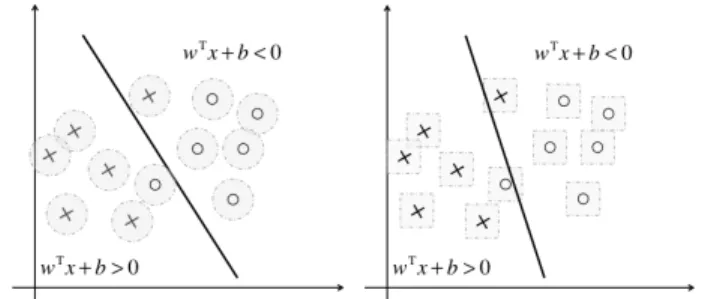
Figure 1: The figures on the left and right illustrates the uncertainty set of each data represented by the
L2-norm and theL∞-norm respectively.
approaches taken when dealing with uncertainty in the data. To entail the uncertainty we assume the uncer-tain data to lie within a bounded set called the uncer-tainty set, and using this we can rewrite (1) into the following robust classification problem.
min w,b,ζ r(w) +C Pm i=1ζi s.t. min δi∈Ui yi(wT(xi+δi) +b)≥1−ζi, ζi≥0 i= 1,· · ·, m, (2)
where (δ1, . . . ,δm) denotes the perturbations of each
data and U =U1× · · · × Um denotes the uncertainty
set for the perturbation of the data.
Usually in robust classification problems, for simplic-ity, we assume all data share an uncorrelated identical uncertainty set, indicating that all data are equally corrupted and uncorrelated [16, 6]. Therefore, the uncertainty set U is expressed as N0× · · · × N0, or otherwise {(δ1, . . . ,δm)|δi ∈ N0}, where N0 denotes the uncertainty set for each perturbations. Figure 1 illustrates two robust classification problems where the uncertainty sets of each data N0 are given as
{δ| kδk2 ≤ γ} and {δ| kδk∞ ≤ γ} respectively. In general, L∞-norm shaped uncertainty sets are used when the perturbation of the features are independent of each other and otherwise L2-norm are used. We will call these uncertainty sets where the pertur-bation of each data are uncorrelated as theconstraint wise uncertainty set, since all data can simultaneously take the worst case perturbations. On the other hand, in such cases as Xu et al. [24], correlated perturbations are considered as well, motivated by the fact that all data realizing the worst case may be too conservative. 2.2 Equivalence to Regularized Classification In this section we show that solving the robust classi-fication is equivalent to solving a regularized classifi-cation. Although many works on robust classifications have been made, their primary focus was on the ex-perimental results they achieved, and not on the
the-oretical equivalence to the standard regularized classi-fication.
Xu et al. [24] were the first to explicitly establish the equivalence between robustness and regulariza-tion. They considered a sublinear aggregated uncer-tainty set, where all the data share an identical uncer-tainty set, but their aggregated behavior is controlled, e.g.,{(δ1, . . . ,δm)|δi∈ N0,Pmi=1kδik ≤γ}. Roughly
speaking, this is different from the constraint wise un-certainty set in that all the data can not take the worst case simultaneously.
We show similar results by considering a constraint wise uncertainty set where each data takes different uncertainty set sizes. Our approach taken to show equivalence between the robust and regularized clas-sifier differs from the methods used in Xu et al. [24]. The most noticeable difference between our work and previous works is that we extended the setting by treating different sizes of uncertainty set for different data. This type of robustness is conveyed in many real life applications where the data are not equally trusted. For example, let each data represent a pa-tient’s health condition, e.g., blood pressures, blood-sugar levels, where the objective is to classify whether a patient is potentially ill or not. If the patients can be examined multiple times and has small measurement variances, we can trust their data. However, if the pa-tients can be examined only for a limited number of time or if they have large measurement variances, we should not trust their data, but instead assume their data belongs to some kind of uncertainty set. In sit-uations like this, rather than assuming that all data share an identical uncertainty set, each data should be treated individually.
The following proposition is the main result of this sec-tion, which shows the equivalence between the robust classification and the regularized classification. Proposition 1 Let Ui = {δi| kδikq ≤ γi} for i ∈
1, . . . , m, and suppose the regularizer r(w) takes the form Pl
k=1ηkkwkdpkk where ηk ≥0, dk, pk ∈ N. Then the following robust classification problem
min w,b,ζ r(w) + Pm i=1Ciζi s.t. min δi∈Ui yi(wT(xi+δi) +b)≥1−ζi, ζi≥0 i= 1,· · · , m, (3)
is equivalent to the following regularized classification problem min w,b,ζ0 r 0(w) +Rkwk p+P m i=1Ci0ζi0 s.t. yi(wTxi+b)≥1−ζi0, ζ0 i≥0 i= 1,· · ·, m, (4)
wherepdenotes the dual norm ofqand the regularizer r0(w)takes the formPl
k=1η 0
kkwk dk
pk. Here, parameters η0k,R and costsCi0 are assigned according to (3).
When we say the two classification problem is “equiv-alent”, we mean they produce the same optimal hy-perplanewTx+b= 0. This result tells us that robust classification problems with different uncertainty set sizes on each data are equivalent to solving a regular-ized classification problem.
We give a brief overview of the proof. For the full version of the proof see the supplementary material. Overview of Proof. Observe that (3) can be rewrit-ten into the following standard (non-robust) optimiza-tion problem. min w,b,ζ r(w) + Pm i=1Ciζi s.t. yi(wTxi+b)−γikwkp≥1−ζi, ζi≥0 i= 1,· · · , m, (5)
wherek · kp is the dual norm ofk · kq.
To show equivalence between (4) and (5), we create an identical optimal hyperplane wTx+b = 0 for (4) and (5) through setting theη0kof the regularizerr0(w), parameterRand costsCi0 appropriately.
Let us first denote the KKT conditions of (5) and (4) as (I) and (II) respectively (see supplementary material). Then let (wrob, brob,ζrob,αrob,βrob) and
(wreg, breg,ζreg0 ,α0reg,βreg0 ) be points satisfying the
KKT conditions (I) and (II) respectively, whereαand βare the dual variables. Since both problems are con-vex, any solution satisfying the KKT conditions is the optimal solution. Therefore, to prove the proposition, we show that we can construct (4) to have an identical optimal hyperplane as wT
robx+brob = 0 that satisfies
the KKT conditions (II), by appropriately setting the
η0k of the regularizerr0(w), parameterRand costsCi0. Letγ= maxiγi. Then for appropriate parametersη0k,
Rand costsCi0, (4) will have an optimal solution satis-fying (wreg, breg) = (τwrob, τ brob), whereτ is defined
asτ =1+γkw1
robkp. Since hyperplanes are invariant
un-der scaling of the parameters, this will be our desired solution.
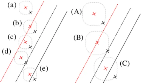
To prove this, we consider two cases; for data with uncertainty set size γ and data with uncertainty set size smaller than γ. Take a look at Figure 2. Black and red are used to illustrate the results of robust and regularized classification respectively. The bold lines represent the optimal hyperplaneswTx+b = 0 and the dashed lines represent the margin hyperplanes
|wTx+b| = 1 for the robust and regularized prob-lems. Finally, the dashed grey circles represent the uncertainty set of each data.
Figure 2: (Left) Data with uncertainty set sizeγi< γ.
(Right) Data with uncertainty set size γi=γ.
Table 1: Description of different types of data in Fig-ure 2. “Others” stands for those data that are cor-rectly classified and not on the margin hyperplane.
Regularized Problem
ME MSV Others
Robust Problem
ME (C), (e) -
-MSV (d) (B)
-Others (c) (b) (A), (a)
The description of the letters in parenthesis is summa-rized in Table 1. Margin Errors (ME) are data with
ζ > 0, Margin Support Vectors (MSV) are data with
ζ= 0 and α >0, and Others denotes data other than ME and MSV, i.e., those data that are correctly clas-sified and not on the margin hyperplane.
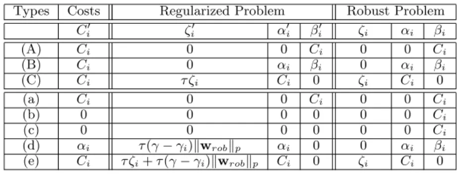
By focusing on the different types of data de-picted in Table 1, we derive a method of con-structing a pair (w, b,ζ,α0,β0) satisfying the KKT conditions (II) where (w, b) = (τwrob, τ brob) using
(wrob, brob,ζrob,αrob,βrob). Table 2 summarizes how
we assign the costsC0
i for each types of data and what
the pairs (ζ0,α0,β0) evaluate to.
Finally, by assigning η0k = ηkτ2−dk, i.e., r0(w) =
Pl
k=1ηkτ2−dkkwkdpkkandR=
Pm
i=1αiγi, we can show
that the above variables {(ζi0, α0i, βi0)}m
i=1 satisfy the KKT conditions (II). Hence proving that the robust classification problem (3) is equivalent to the regular-ized classification problem (4) if theηk0 of the regular-izer r0(w), parameter R and costs Ci0 are assigned in the above manner.
To get a better understanding of Proposition 1 we pro-vide the following corollary. It reveals that the stan-dardC-SVM is equivalent to a non-regularized robust classification, and provides theoretical explanation on why C-SVMs are robust to data. By substituting
Ci = 1, γi = γ for i = 1, . . . , m and r(w) = 0 in
Table 2: Relationship between the assigned costs and the optimal solutions. Types Costs Regularized Problem Robust Problem
Ci0 ζi0 α0i βi0 ζi αi βi (A) Ci 0 0 Ci 0 0 Ci (B) Ci 0 αi βi 0 αi βi (C) Ci τ ζi Ci 0 ζi Ci 0 (a) Ci 0 0 Ci 0 0 Ci (b) 0 0 0 0 0 0 Ci (c) 0 0 0 0 0 0 Ci (d) αi τ(γ−γi)kwrobkp αi 0 0 αi βi (e) Ci τ ζi+τ(γ−γi)kwrobkp Ci 0 ζi Ci 0
Corollary 1 Let U = {δ| kδkq ≤ γ}. Then the
fol-lowing two classification problems are equivalent.
min w,b,ζ Pm i=1ζi s.t. min δi∈U yi(wT(xi+δi) +b)≥1−ζi, ζi≥0 i= 1,· · ·, m, (6) min w,b,ζ0 Rkwkp+ Pm i=1ζ 0 i s.t. yi(wTxi+b)≥1−ζi0, ζi0≥0 i= 1,· · · , m, (7)
where pdenotes the dual norm of q and parameter R is assigned according to (6).
Proof. We first show that for any robust problem (6), there exists a regularized problem (7) that pro-duces an identical optimal hyperplane. Since every data has an identical uncertainty set, we only con-sider data of Type (A), (B) and (C). Looking at Table 2, we can assign costs Ci0 = 1 for every data since
Ci = 1. Therefore, by substituting R = Pmi=1αiγi,
where αi are the corresponding dual variables of the
robust problem, we obtain (7). The other side of the statement is easily proven using the above result. If we assign, γ=R/Pm
i=1α0i, whereα0i are the
correspond-ing dual variables of the regularized problem, (6) will achieve the same optimal hyperplane as (7). By substitutingq= 2, we obtain the standardC-SVM. Although the regularizerRkwk2is degree 1, it is easily confirmed that it produces the same optimal hyper-plane as the standard C-SVM where the regularizer is 1
2kwk 2
2 by setting R properly. We note the state-ment in Corollary 1 slightly differs from Proposition 1. While in Corollary 1, strict equivalence between the robust and regularized classification was shown, in Proposition 1 we have not stated that any regularized classification is equivalent to a robust classification. Finally, we briefly explain how to handle the multi pa-rametersCi andγiin Proposition 1 in practice, which
are too costly to tune individually using grid search. We provide an example on how we can tune Ci and
γi appropriately from prior knowledge, using the
pre-vious example of classifying a patient as potentially ill or not. If the classes are imbalanced,Ci can be tuned
to be the imbalanced ratio of the two classes. For the
γi, we can set them as the variance of the examined
data. This allows us to convey the uncertainty or vari-ance of each patient’s examined data, which is more appropriate to obtain robust solutions than training the model against the average of the examined data. In other cases whereCiandγiare assumed to have no
significant differences between patients, we can assign them identical values to obtain a model with smaller number of parameters.
3
Connections To Existing
Classifications
3.1 Robust Classification of Xu et al.
In the previous section, we showed equivalence be-tween the non-regularized robust classification and the standardC-SVM. This was also observed by Xu et al. [24] in a different robust setting. In this section, we look into the connection with their results and observe that our result can be considered as a generalization of theirs.
While we considered a constraint wise uncertainty set {(δ1, . . . ,δm)| δi ∈ N0}, Xu et al. [24] con-sidered a sublinear aggregated uncertainty set, e.g.,
{(δ1, . . . ,δm)| δi ∈ N0,P
m
i=1kδik ≤ γ}. Roughly
speaking, the sublinear aggregated uncertainty set re-stricts the data of simultaneously achieving the worst case by controlling the aggregated behavior of the per-turbation. Their main purpose for considering this was to obtain a less conservative solution than the constraint wise uncertainty set. However, our result shows that a sublinear aggregated uncertainty set can be replicated by a small sized constraint wise uncer-tainty set. We also point out that while they need an assumption of the data being non-separable, our result holds for any type of data set.
We begin by introducing the main result of Xu et al. [24] following their definition with minor alteration in the notations.
Theorem 1 (Theorem 3 of Xu et al.) Let T =
{(δ1, . . . ,δm)| P m
i=1kδikq ≤ γ0}. Suppose that the
training data are non-separable. Then the following two classification problems are equivalent.
min w,b,ζ Pm i=1ζi s.t. min δi∈T yi(wT(xi+δi) +b)≥1−ζi, ζi ≥0 i= 1,· · · , m, (8) min w,b,ζ0 γ 0kwk p+P m i=1ζi0 s.t. yi(wTxi+b)≥1−ζi0, ζi0≥0 i= 1,· · ·, m, (9)
wherepdenotes the dual norm of q.
Although for simplicity we refrain ourselves from pro-viding the definition of sublinear aggregated uncer-tainty sets, the following argument holds for any sub-linear aggregated uncertainty set.
It can be seen from Theorem 1 that Xu et al. [24] considers an uncertainty set where the perturbation of the data are correlated. Furthermore, (9) in Theorem 1 is the same form as (7) in Corolallry 1. Therefore, by substituting R=γ0, we can conclude that (6) and (8) are equivalent robust classification problems. In addition, from the assumption in Theorem 1 that the data are non-separable, at least one of the dual variable
αi in (6) equals to 1, leading toR =γP m
i=1αi > γ.
Thusγ0> γ.
From the above argument, we see that the sublin-ear aggregated uncertainty set is replicated by a con-straint wise uncertainty set where the perturbation on each data are smaller, i.e., γ < γ0. This implies that even though considering the sublinear aggregated un-certainty set seems to be less conservative by control-ling the perturbation through aggregate constraints, it is actually equivalent to considering a small sized constraint wise uncertainty set where every data can simultaneously take the worst case.
3.2 Elastic Net SVM
The Elastic Net SVM, also known as the Doubly Reg-ularized SVM was first proposed by Wang et al. [22], and several efficient algorithms have been proposed since then [25, 4]. The EN-SVM uses a mixture of
L1-norm and L2-norm regularizer, i.e., the elastic net regularizer, where the L1-norm promotes sparsity of the optimal solution andL2helps groups of correlated variables to get selected.
In this section we present an equivalent formulation to the EN-SVM and give an alternative explanation on the properties of the elastic net regularizer. Let us observe the following corollary.
Corollary 2 Let T2 = {δ| kδk2 ≤ γ} and T∞ =
{δ0| kδ0k∞ ≤ γ0}. Then the following three
classifi-cation problems are equivalent.
min w,b,ζ Pm i=1ζi s.t. min δi∈T2+T∞ yi(wT(xi+δi) +b)≥1−ζi, ζi≥0 i= 1,· · · , m. (10) min w,b,ζ0 Ckwk 2 2+ Pm i=1ζ 0 i s.t. min δi∈T∞ yi(wT(xi+δi) +b)≥1−ζi0, ζi0≥0 i= 1,· · ·, m, (11) min w,b,ζ00 λ2 2kwk 2 2+λ1kwk1+Pmi=1ζi00 s.t. yi(wTxi+b)≥1−ζi00, ζi00≥0 i= 1,· · ·, m. (12)
Equivalence between (11) and (12) is shown in the same manner as Corollary 1. This states that EN-SVM (12) is equivalent to a robustC-SVM (11) where the perturbation is given as a L∞-norm uncertainty set. In other words, aL∞-norm uncertainty set on the data has the effect of promoting a sparse hyperplane. This can be understood intuitively since a L∞-norm uncertainty set is shaped like a box where the sides are parallel to the axes. Therefore, by considering a L∞ -norm uncertainty set on the perturbation, the robust
C-SVM will learn according to theL2-norm regularizer but at the same time try to create a sparse hyperplane. Furthermore, equivalence between (10) and (11) is ob-tained directly from the result of Corollary 1. Thus, EN-SVM is equivalent to a non-regularized SVM with uncertainty set δEN ∈ T2+T∞ = {δ+δ0| kδk2 ≤
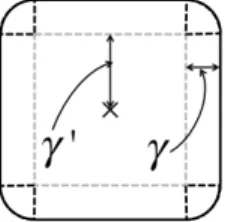
γ,kδ0k∞ ≤γ0}. This uncertainty set is shaped like a box with circular corners as depicted in Figure 3. Asγ
becomes larger it will shape more like a circle, and as
γ0 becomes larger it will shape more like a box. This figure provides an alternative explanation on the prop-erties of the elastic net regularizer and suggests that there might be a method of tuning the parametersλ1 andλ2 through a robust optimization perspective.
4
Application: Imbalanced Data
Learning
In general, robust optimizations are used to incorpo-rate the uncertainty and ambiguity of the data by assigning some sort of uncertainty set around them.
Figure 3: Uncertainty set that realizes the Elastic Net regularization. γ and γ0 denotes the size of the L2 -norm andL∞-norm uncertainty set respectively.
However, as we saw in Proposition 1, robust classifi-cation problems can also be viewed as a cost sensitive model. Unlike in the usual cost sensitive classification models [15, 3, 21] where the costs are assigned accord-ing to the classes, in the robust classification models the costs are essentially assigned according to the dual variablesζ of the data, i.e., the amount of misclassifi-cation error of a certain data.
In this section we compare the robust classification model with other standard cost sensitive methods against imbalanced data sets, and see that assigning costs in the above manner provides a competitive so-lution to other existing methods. Furthermore, we see that considering a larger uncertainty set around the minority class has the effect of oversampling. This is a novel usage of the robust classification scheme and the results show that it applies well with imbalanced data learning.
4.1 Proposed Algorithm RCSSVM
We introduce two non-regularized robust cost sensi-tive SVMs (RCSSVM) where the uncertainty sets are given as the L2-norm and the L∞-norm. The objec-tive function of RCSSVM only consists of the loss term
C+P
iζi+C−Pjζj, where the summation on the left
and right are taken respectively to the data in the mi-nority class and majority class. Since the optimal hy-perplane is invariant to multiplication of the objective function, we setC−= 1. For the constraint, we assign two different uncertainty sets for the minority and ma-jority class. In detail, the constraint of RCSSVM-L∞ is equivalent to that of (3) where two uncertainty sets
U+ and U− are considered. U+ and U− denote the uncertainty sets for the minority class and majority class respectively, and are defined as{δ| kδk∞≤γ+} and{δ| kδk∞≤γ−}whereγ+is assigned larger than
γ−. The intuition behind this is that since the mi-nority class has less data compared to the majority class, we consider the minority class to be less credible. Figure 4 explains the effect of considering uncertainty sets of different sizes. As it can be seen, considering a larger uncertainty set for the minority class copes
Figure 4: Example of RCSSVM-L2. The x and o de-note the minority and majority classes respectively, and the grey areas represent their uncertainty sets. Table 3: The datasets used for experimentation. The number after the dataset names indicates the minor-ity class we used. Those without numbers are binary classification.
Dataset Instances Ratio Features breast cancer 699 1:2 11 hepatitis1 155 1:4 19 glass7 214 1:6 9 segment1 2310 1:6 19 ecoli 336 1:8.6 7 arrhythmia6 452 1:11.8 279 soy bean15 683 1:15 35 sick2 3772 1:15 29 oil spill 937 1:21.9 49 car4 1728 1:25.6 6 yeast5 1433 1:27 8 hypothyroid3 3772 1:39 52 abalone19 4145 1:130 8
for the lack of data, since the problem tries to learn all the data inside the uncertainty sets. Alternatively, RCSSVM can be thought as oversampling the minor-ity class. RCSSVM-L2is defined in the same manner where k · k2 is used instead ofk · k∞.
4.2 Dataset
To evaluate the classification performance of our pro-posed algorithm, we used 13 datasets from the UCI database with different degrees of imbalance. The datasets used are listed in Table 3. The multiclass datasets were converted into binary datasets using the one-versus-all scheme. The imbalance ratio var-ied from 1:2 to 1:130.
4.3 Experiment
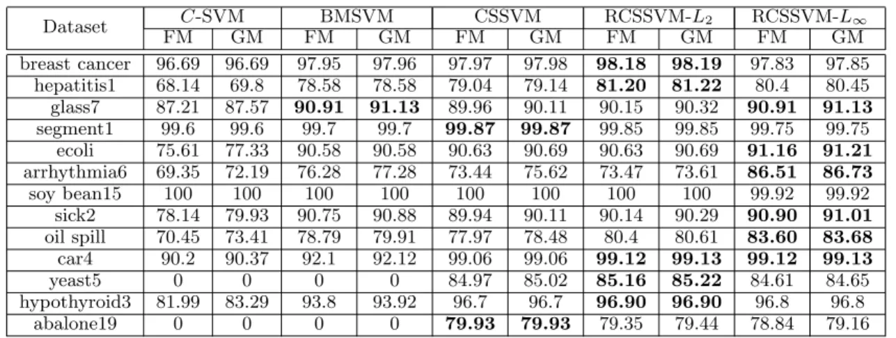
In our experiment, we compared RCSSCVMs with other basic methods: C-SVM, boundary movement SVM (BMSVM) [17] and cost sensitive SVM (CSSVM) [15, 3, 21]. Both BMSVM and CSSVM are algo-rithms that modify C-SVM. BMSVM shifts the deci-sion boundary by adjusting the threshold of C-SVM, and CSSVM penalizes differently between the minority
Table 4: Experimental results for all the methods. Dataset C-SVM BMSVM CSSVM RCSSVM-L2 RCSSVM-L∞ FM GM FM GM FM GM FM GM FM GM breast cancer 96.69 96.69 97.95 97.96 97.97 97.98 98.18 98.19 97.83 97.85 hepatitis1 68.14 69.8 78.58 78.58 79.04 79.14 81.20 81.22 80.4 80.45 glass7 87.21 87.57 90.91 91.13 89.96 90.11 90.15 90.32 90.91 91.13 segment1 99.6 99.6 99.7 99.7 99.87 99.87 99.85 99.85 99.75 99.75 ecoli 75.61 77.33 90.58 90.58 90.63 90.69 90.63 90.69 91.16 91.21 arrhythmia6 69.35 72.19 76.28 77.28 73.44 75.62 73.47 73.61 86.51 86.73 soy bean15 100 100 100 100 100 100 100 100 99.92 99.92 sick2 78.14 79.93 90.75 90.88 89.94 90.11 90.14 90.29 90.90 91.01 oil spill 70.45 73.41 78.79 79.91 77.97 78.48 80.4 80.61 83.60 83.68 car4 90.2 90.37 92.1 92.12 99.06 99.06 99.12 99.13 99.12 99.13 yeast5 0 0 0 0 84.97 85.02 85.16 85.22 84.61 84.65 hypothyroid3 81.99 83.29 93.8 93.92 96.7 96.7 96.90 96.90 96.8 96.8 abalone19 0 0 0 0 79.93 79.93 79.35 79.44 78.84 79.16
and majority class by assigning different costs. All ex-periments were conducted by 10-fold cross-validation and the training/test subsets were created by strat-ified sampling to ensure each subset had the same ratio of minority and majority class data. For all methods, the parameters C, C+, γ+, γ− were selected through grid search. The range of C was [10−5,105], the range ofC+was [1,5×Imbalance Ratio]. The grid forγ+andγ−were [10−3,10−1] satisfying the inequal-ity γ+> γ−.
To evaluate the quality of the classifiers, we used f-measure [14, 9] and g-means [12, 1], which are evalu-ation metrics defined as P2P R+R and √P R respectively, whereP andRdenote the precision and recall. These evaluation metrics are commonly used in imbalanced data learning, since evaluating the performance of a classifier by the overall accuracy is irrelevant. The re-sult is summarized in Table 4. The table shows that both RCSSVMs outperform theC-SVM, BMSVM and CSSVM in most cases. It can be seen that compared to theC-SVM, both RCSSVMs learn significantly bet-ter on imbalanced data and the results encourage that RCSSVMs are suitable for imbalanced data learning. We now point out an interesting property of
RCSSVM-L∞. For the two datasets “arrhythmia6” and “oil spill” that have high numbers of features,
RCSSVM-L∞ learns significantly better than the other meth-ods. This is probably due to the fact that the datasets include features that are unnecessary or redundant. Since RSCSVM-L∞ considers box-shaped uncertainty sets around the data, it automatically performs feature selections, whereas the other methods try to learn all features. Owing to this, every solution obtained by the RCSSVM-L∞created a sparse optimal hyperplane. It should also be noted that compared to other methods, RCSSVM-L∞ was computationally much lighter than other methods, owing to the fact that it solves a linear programing problem.
5
Conclusions
We investigated the relationship between the robust and regularized SVM classification. Unlike previous robust classification models, we allowed uncertainty sets to be of different sizes for each data, and made it possible for the model to incorporate different un-certainties and ambiguities of the data. The obtained result presents that having some norm-based pertur-bation around the data is equivalent to considering a norm-based regularizer and gives theoretical explana-tion on why regularized classifiers tend to be robust against data. Furthermore, we showed that the stan-dard (non-robust) SVM and the elastic net SVM pro-vide solutions to robust classification problems where the uncertainty sets are the L2-norm and a combina-tion of theL2-norm andL∞-norm respectively. In consideration of the above result, we showed that robust classification models could be applied to cost sensitive learning. The presented model has been in-vestigated for some benchmark imbalanced data and the experimental results have demonstrated that the robust classification model provides a promising poten-tial for imbalanced data learning. The interpretation of this is that setting a larger uncertainty set on the minority class has an effect of oversampling and copes for the lack of data. For our proposed method we used the L2-norm and L∞-norm uncertainty set and observed that the L∞-norm uncertainty set achieves automatic feature selection.
In future research we will investigate how to construct uncertainty sets that best suit the problem. Further-more, in this paper we were only able to conduct ex-periments on class-wise RCSSVM, since we could not find suitable data that expressed each sample’s uncer-tainty. Therefore, it is also a great interest for us to find a well suited data and experiment using RCSSVM where the costs are assigned individually.
References
[1] Rehan Akbani, Stephen Kwek, and Nathalie Jap-kowicz. Applying support vector machines to im-balanced datasets. In Machine Learning: ECML 2004, pages 39–50. Springer, 2004.
[2] Martin Anthony and Peter L Bartlett. Neural network learning: Theoretical foundations. cam-bridge university press, 2009.
[3] Francis R Bach, David Heckerman, and Eric Horvitz. Considering cost asymmetry in learn-ing classifiers. The Journal of Machine Learning Research, 7:1713–1741, 2006.
[4] P Balamurugan. Large-scale elastic net regu-larized linear classification svms and logistic re-gression. In Data Mining (ICDM), 2013 IEEE 13th International Conference on, pages 949–954. IEEE, 2013.
[5] Aharon Ben-Tal, Laurent El Ghaoui, and Arkadi Nemirovski. Robust optimization. Princeton Uni-versity Press, 2009.
[6] Aharon Ben-Tal, Arkadi Nemirovski, and Cees Roos. Robust solutions of uncertain quadratic and conic-quadratic problems. SIAM Journal on Optimization, 13(2):535–560, 2002.
[7] Chiranjib Bhattacharyya, KS Pannagadatta, and Alexander J Smola. A second order cone program-ming formulation for classifying missing data. In
Neural Information Processing Systems (NIPS), pages 153–160, 2005.
[8] Bernhard E Boser, Isabelle M Guyon, and Vladimir N Vapnik. A training algorithm for op-timal margin classifiers. InProceedings of the fifth annual workshop on Computational learning the-ory, pages 144–152. ACM, 1992.
[9] Nitesh V Chawla, David A Cieslak, Lawrence O Hall, and Ajay Joshi. Automatically counter-ing imbalance and its empirical relationship to cost. Data Mining and Knowledge Discovery, 17(2):225–252, 2008.
[10] Corinna Cortes and Vladimir Vapnik. Support-vector networks. Machine learning, 20(3):273– 297, 1995.
[11] Laurent El Ghaoui and Herv´e Lebret. Robust so-lutions to least-squares problems with uncertain data. SIAM Journal on Matrix Analysis and Ap-plications, 18(4):1035–1064, 1997.
[12] Miroslav Kubat, Stan Matwin, et al. Addressing the curse of imbalanced training sets: one-sided selection. In ICML, volume 97, pages 179–186. Nashville, USA, 1997.
[13] Gert RG Lanckriet, Laurent El Ghaoui, Chiranjib Bhattacharyya, and Michael I Jordan. A robust minimax approach to classification. The Journal of Machine Learning Research, 3:555–582, 2003. [14] David D Lewis and Marc Ringuette. A
compari-son of two learning algorithms for text categoriza-tion. In Third annual symposium on document analysis and information retrieval, volume 33, pages 81–93, 1994.
[15] Yi Lin, Yoonkyung Lee, and Grace Wahba. Sup-port vector machines for classification in nonstan-dard situations. Machine Learning, 46(1-3):191– 202, 2002.
[16] Miguel Sousa Lobo, Lieven Vandenberghe, Stephen Boyd, and Herv´e Lebret. Applications of second-order cone programming. Linear alge-bra and its applications, 284(1):193–228, 1998. [17] Grigoris Karakoulas John Shawe-Taylor.
Opti-mizing classifiers for imbalanced training sets. In
Advances in Neural Information Processing Sys-tems 11: Proceedings of the 1998 Conference, vol-ume 11, page 253. MIT Press, 1999.
[18] Pannagadatta K Shivaswamy, Chiranjib Bhat-tacharyya, and Alexander J Smola. Second order cone programming approaches for handling miss-ing and uncertain data. The Journal of Machine Learning Research, 7:1283–1314, 2006.
[19] Theodore B Trafalis and SA Alwazzi. Robust optimization in support vector machine training with bounded errors. In Neural Networks, 2003. Proceedings of the International Joint Conference on, volume 3, pages 2039–2042. IEEE, 2003. [20] Theodore B Trafalis and Robin C Gilbert.
Ro-bust support vector machines for classification and computational issues. Optimisation Methods and Software, 22(1):187–198, 2007.
[21] Konstantinos Veropoulos, Colin Campbell, Nello Cristianini, et al. Controlling the sensitivity of support vector machines. In Proceedings of the international joint conference on artificial intelli-gence, volume 1999, pages 55–60, 1999.
[22] Li Wang, Ji Zhu, and Hui Zou. The doubly regu-larized support vector machine. Statistica Sinica, 16(2):589, 2006.
[23] Huan Xu, Constantine Caramanis, and Shie Man-nor. Robust regression and lasso. In Advances in Neural Information Processing Systems, pages 1801–1808, 2009.
[24] Huan Xu, Constantine Caramanis, and Shie Man-nor. Robustness and regularization of support vector machines. The Journal of Machine Learn-ing Research, 10:1485–1510, 2009.
[25] Gui-Bo Ye, Yifei Chen, and Xiaohui Xie. Efficient variable selection in support vector machines via the alternating direction method of multipliers. In International Conference on Artificial Intelli-gence and Statistics, pages 832–840, 2011.