Titl e Ti m e S e r i e s I m p u t a ti o n vi a L1 N o r m-B a s e d Si n g ul a r S p e c t r u m An aly si s Ty p e Ar ticl e U RL h t t p s :// u al r e s e a r c h o nli n e . a r t s . a c . u k/i d/ e p ri n t/ 1 2 5 7 4 / D a t e 2 0 1 8 Cit a ti o n K al a n t a r i, Y a n d Yar m o h a m m a d i, M a n d H a s s a n i, H . a n d Silv a, E . S. ( 2 0 1 8 ) Ti m e S e r i e s I m p u t a ti o n vi a L1 N o r m-B a s e d Si n g u l a r S p e c t r u m An aly si s. Fl u c t u a ti o n a n d N oi s e L e t t e r s , 1 7 ( 2). C r e a t o r s K al a n t a r i, Y a n d Yar m o h a m m a d i, M a n d H a s s a n i, H . a n d Silv a, E . S. U s a g e G u i d e l i n e s Pl e a s e r ef e r t o u s a g e g u i d eli n e s a t
h t t p :// u al r e s e a r c h o n li n e . a r t s . a c . u k / p olici e s . h t m l o r a l t e r n a tiv ely c o n t a c t
u a l r e s e a r c h o n li n e @ a r t s . a c . u k.
Lic e n s e : C r e a tiv e C o m m o n s Att ri b u ti o n N o n-c o m m e r ci al N o D e riv a tiv e s U nl e s s o t h e r wi s e s t a t e d , c o p y ri g h t o w n e d b y t h e a u t h o r
Time Series Imputation via
L
1
Norm based
1
Singular Spectrum Analysis
2Mahdi Kalantari
∗, Masoud Yarmohammadi
∗, Hossein Hassani
†and
Emmanuel Sirimal Silva
‡∗Department of Statistics, Payame Noor University, 19395–4697, Tehran, Iran.
†Research Institute of Energy Management and Planning, University of Tehran, Iran
‡Fashion Business School, London College of Fashion, University of the Arts London, UK
3
Abstract
4
Missing values in time series data is a well-known and important problem which 5
many researchers have studied extensively in various fields. In this paper, a new 6
nonparametric approach for missing value imputation in time series is proposed. 7
The main novelty of this research is applying theL1 norm based version of Singular
8
Spectrum Analysis (SSA), namely L1-SSA which is robust against outliers. The
9
performance of the new imputation method has been compared with many other 10
established methods. The comparison is done by applying them to various real and 11
simulated time series. The obtained results confirm that the SSA based methods, 12
especially L1-SSA can provide better imputation in comparison to other methods.
13
Keywords: Time Series, Basic SSA, L1-SSA, Reconstruction, Missing value,
Im-14
putation. 15
1 Introduction
16When dealing with real-world situations, missing values are commonly encountered in
17
time series due to many reasons such as instrument malfunctions or failures to record
18
observations, human mistakes and lost records. Eliminating those values may result in
19
the loss of key information relevant to the inference. Imputation, which is the estimation of
20
missing values, is an important part of the data cleaning process in time series analysis [1].
21
Most statistical analysis tools could be used after the imputation of missing values. It
22
is noteworthy that imputing missing values alters the original time series; consequently,
23
wrong imputation can severely affect the forecasting performance [2]. To this end, some
24
authors believe that the treatment of missing observations can be more important than
25
the choice of forecasting method [1]. Hence, employing effective and sound imputing
26
algorithms to obtain the best possible imputes is of great importance. Missing data also
27
prevents the production of statistically reliable statements about the variables and often
28
further data analysis steps rely on complete data sets.
29
Imputation is a widespread area in time series analysis and some methods have been
30
developed for imputing in time series. Examples of some traditional methods can be
31
found in [3–7].
Choosing the proper imputing technique depends on the structure of time series
con-33
cerned. Different series may require different strategies to impute missing values. An
34
Expectation-Maximisation (EM) algorithm based method for imputation of missing
val-35
ues in multivariate normal time series has been proposed in [8]. This imputation algorithm
36
accounts for both spatial and temporal correlation structures [9]. State-space
represen-37
tation or Kalman filter approach is another suitable method used for imputing, see [10]
38
for more details. The use of ARIMA and SARIMA models for imputation of univariate
39
time series was evaluated in [11]. The missing value estimation in the context of additive
40
outliers and influential observations in time series can be found in [12, Chap. 6]. For
max-41
imum likelihood fitting of ARMA models and estimation of ARIMA models with missing
42
values see [13, 14].
43
A major drawback of standard imputation methods in time series is assuming
sta-44
tionarity for the data, linearity for the model or normality for the errors which can only
45
provide an approximation to the real situation. One solution for overcoming these
diffi-46
culties is via the employment of nonparametric approaches. Given the advantage of not
47
being restricted by any of the parametric assumptions enables nonparametric methods
48
to provide a much closer representation of the real world scenario [15]. As such,
non-49
parametric methods are extensively used in statistical analyses. The Singular Spectrum
50
Analysis (SSA) technique is a very good example of such methods. Applications of this
51
powerful and nonparametric technique is increasingly wide spread in time series analysis
52
and other fields; for references see e.g. [15–19].
53
Interestingly, one of the effective applications of SSA is imputation in time series.
54
Some methods for imputation based on SSA have been designed for stationary time series
55
[20, 23] whilst in [21] a more general approach which is applicable to different kinds of
56
time series was proposed. An extension of SSA forecasting algorithms for gap filling was
57
proposed in [24]. In this subspace approach, the structure of the extracted component
58
is continued to the gaps caused by the missing values. In another gap filling method
59
proposed in [25], a weighted combination of the forecasts and hindcasts yielded by the
60
recurrent SSA forecasting algorithm was used. This approach was further enhanced by
61
using bootstrap re-sampling and a weighting scheme based on sample variances in [26].
62
In this paper, we propose a new approach for missing data imputation in
univari-63
ate time series within the SSA framework. In this method, missing values are replaced
64
by initial values and then reconstructed repeatedly until convergence occurs. The last
65
reconstructed values are considered as imputed values. It is noteworthy that the idea
66
underlying the iterative algorithm was derived from [21] and was in fact suggested earlier
67
for imputation of gaps in matrices in [22]. The main novelty of the proposed technique
68
is its application of the L1 norm based version of SSA, namely L1-SSA which was
intro-69
duced in [27]. Recall that the basic version of SSA is based on the Frobenius norm orL2
70
norm. The main advantages of this newly proposed approach are its robustness against
71
outliers and lack of assumptions relating to the stationarity of time series and normality of
72
random errors. The results from the proposed method are compared with those attained
73
via other established methods such as Interpolation, Kalman Smoothing and Weighted
74
Moving Average. The obtained results confirm that the SSA based methods, especially
75
L1-SSA can provide better imputation in comparison to other methods.
76
The remainder of this paper is organised as follows. A brief introduction into L1-SSA
77
and the new imputation method are given in Section 2. The other imputation methods are
78
presented in Section 3 in more detail. In addition, this section also evaluates the
mance of imputation methods via applications which compare them with simulated and
80
real time series. Finally, Section 4 presents a summary of the study and some concluding
81
remarks.
82
2 New Imputation Method
83In this section; first, a short description of L1-SSA is presented. Thereafter, we propose
84
the new imputation method based on L1-SSA.
85
2.1 A Brief Description of
L
1-SSA
86
The SSA technique consists of two complementary stages: Decomposition and
Reconstruc-87
tion, and both of these include two separate steps [28]. At the first stage we decompose
88
the series in order to enable signal extraction and noise reduction. At the second stage we
89
reconstruct a less noisy series and use the reconstructed series for forecasting new data
90
points [19]. The theory underlying SSA is explained in more detail in [28]. The most
91
common version of SSA is called Basic SSA [28]. It is notable that the matrix norm used
92
in Basic SSA is theFrobeniusnorm orL2-norm. Recently, a newer version of SSA which is
93
based onL1-norm and therefore called L1-SSA was introduced and it was confirmed that
94
L1-SSA is robust against outliers [27]. In the following, the steps ofL1-SSA are concisely
95
presented. For more detailed information onL1-SSA, see [27].
96
Stage 1: Decomposition
97
LetYN ={y1, . . . , yN} be the time series and L (2≤ L < N−1) be some integer called
98
the window length.
99
Step 1: Embedding 100
In this step; firstly, the lagged vectorsof size Lare built as follows:
Xi = (yi, . . . , yi+L−1)T, 1≤i≤K,
whereK =N−L+ 1. Secondly, thetrajectory matrix of the time series YN is defined as:
X= [X1 :· · ·:XK] = (xij)L,Ki,j=1 = y1 y2 y3 . . . yK y2 y3 y4 . . . yK+1 y3 y4 y5 . . . yK+2 .. . ... ... . .. ... yL yL+1 yL+2 . . . yN
Note thatXhas equal elements on theanti-diagonals i+j =const. Matrices of this type
101
are called Hankel matrices.
Step 2: Singular Value Decomposition (SVD) 103
In this step, the Singular Value Decomposition (SVD) of the trajectory matrix X is performed. Suppose that λ1, . . . , λL are the eigenvalues of XXT taken in the decreasing
order of magnitude (λ1 ≥ · · · ≥λL≥0) andU1, . . . , UL are theeigenvectorsof the matrix
XXT corresponding to these eigenvalues. Setd=rankX =max{i,such thatλ
i >0}, the
number of positive eigenvalues. If we denote Vi =XTUi/
√
λi (i= 1, . . . , d), the SVD of
the trajectory matrixX in L1-SSA can be written as:
X=X1+· · ·+Xd= d ∑ i=1 wi √ λiUiViT, where Xi = wi √
λiUiViT. The wi is the weight of singular value
√
λi. These weights
104
are diagonal elements of diagonal weight matrixW=diag(w|1, w2{z, . . . , w}d d ,0,0, . . . ,0 | {z } L−d )and 105
are computed such that X−UWΣVTL
1 is minimized; where U = [U1 : · · · : UL], 106 V = [V1 :· · ·: VL], Σ=diag( √ λ1, √ λ2, . . . , √
λL) and ∥.∥L1 is the L1 norm of a matrix. 107
For more information, see [27].
108
Stage 2: Reconstruction
109
Step 3: Grouping 110
In this step, we partition the set of indices {1, . . . , d} into m disjoint subsets I1, . . . , Im.
111
Let I = {i1, . . . , ip}. Then the matrix XI corresponding to the group I is defined as
112
XI =Xi1 +· · ·+Xip. For example, if I ={1,2,7} then XI =X1+X2 +X7. In signal
113
extraction problems, r leading eigentriples are chosen. That is, indices {1, . . . , d} are
114
partitioned into two subsets I1 ={1, . . . , r} and I2 ={r+ 1, . . . , d}.
115
Step 4: L1-Hankelization
116
In this step, we seek to transform each matrix XIj of the grouping step into a Hankel
117
matrix so that these can subsequently be converted into a time series, which is an additive
118
component of the initial seriesYN. LetHAbe the result of the Hankelization of matrixA.
119
In L1-SSA, Hankelization corresponds to computing the median of the matrix elements
120
over the “antidiagonal”. This type of Hankelization has an optimal property in the sense
121
that the matrixHA is the nearest toA (with respect to the L1 norm) among all Hankel
122
matrices of the same dimension [27]. On the other hand, ∥A− HA∥L1 is minimum; so 123
this type of Hankelization is denoted byL1-Hankelization.
124
L1-Hankelization applied to a resultant matrix XIj of the grouping step, produces a
reconstructed seriesYeN(j) ={ye(j)1 , . . . ,ye(j)N }. Therefore, the initial seriesYN ={y1, . . . , yN}
is decomposed into a sum of m reconstructed series:
yt= m ∑ j=1 e yt(j), t = 1,2, . . . , N.
2.2 New Imputation Algorithm Based on
L
1-SSA
125Prior to presenting the algorithm, we find it pertinent to clarify that we do not change the
126
L2-norm toL1-norm during the construction of projectors. Instead, this change occurs at
127
the Hankelization step. Thus, the decomposition stage results in a correction of the L2
128
decomposition and is therefore in reality, a L1-L2 decomposition.
129
Let YN(i) ={y1, . . . , yi−1, ⋆, yi+1, . . . , yN} be the time series where only theith value is
130
missing (i= 1, . . . , N). The symbol ’⋆’ stands for the missing value and it is obvious that
131
iis the position of this value. In the iterative L1-SSA imputation method, missing values
132
are replaced by initial values and then reconstructed repeatedly until convergence occurs,
133
as proposed in [21]. The last reconstructed values are considered as imputed values. This
134
imputation algorithm contains the following steps:
135
Step 1) Set a suitable initial value in place of missing data.
136
Step 2) Choose reasonable values ofL and r.
137
Step 3) Reconstruct the time series where its missing data is replaced with a number.
138
Step 4) Replace theith value of time series with its ith reconstructed value.
139
Step 5) Repeat steps 3 and 4 until the absolute value of the difference between successive
140
replaced values of the time series by their reconstructed value is less than δ. (δ 141
is the convergence threshold.)
142
Step 6) Consider the final replaced value as the imputed value.
143
3 Empirical Results
144In this section; firstly, the other imputation methods are briefly discussed. Secondly, the
145
comparison criteria which are used in this paper are defined. Thirdly, the performance
146
of algorithms for imputation of one missing value are compared via a simulation study.
147
Finally, all of the imputation methods are assessed by applying them to real data.
148
3.1 Other Imputation Methods
149
The other imputation algorithms of univariate time series which are used in this paper
150
are as follows:
151
1. Iterative Basic SSA: In this method, the imputation algorithm proposed in Section
152
2.2 is used for imputation via Basic SSA.
153
2. Interpolation: Linear, spline and Stineman interpolation are used to impute missing
154
values.
155
3. Kalman Smoothing: The Kalman smoothing on the state space representation of an
156
ARIMA model is used for imputation.
157
4. LOCF: Each missing value is replaced with the most recent present value prior to
158
it (Last Observation Carried Forward).
5. NOCB:The LOCF is done from the reverse direction, starting from the back of the
160
series (Next Observation Carried Backward).
161
6. Weighted Moving Average: Missing values are replaced by its weighted moving
162
average. The average in this implementation is taken from an equal number of
163
observations on either side of a missing value. For example, for imputation of missing
164
value at location i, the observations yi−2, yi−1, yi+1, yi+2, are used to calculate the
165
mean for moving average window size 4 (2 left and 2 right). The moving average
166
window size 8 (4 left and 4 right) is taken into account in this paper. The weighted
167
moving average is used in the following three ways:
168
• Simple Moving Average (SMA):All observations in the moving average window
169
are equally weighted for calculating the mean.
170
• Linear Weighted Moving Average (LWMA): Weights decrease in arithmetical
171
progression. The observations directly next to theith missing value (yi−1, yi+1)
172
have weight 1/2, the observations one further away (yi−2, yi+2) have weight 1/3,
173
the next yi−3, yi+3 have weight 1/4 and so on.
174
• Exponential Weighted Moving Average (EWMA): Weights decrease
exponen-175
tially. The observations directly next to the ith missing value have weight 1 21, 176
the observations one further away have weight 1
22, the next have weight 213 and 177
so on.
178
In SSA based imputation methods (Basic SSA and L1-SSA), for reconstruction of
179
simulated series in Section 3.3, the number of leading eigenvalues (r) have been selected
180
according to the rank of the corresponding trajectory matrix. All calculations of
imputa-181
tion methods (except SSA) are done with the help of theR package imputeTS. For more
182
information see [29]. For Basic SSA computations, theR packageRssa is employed. For
183
more details see [30–32].
184
3.2 Comparing Criteria
185
In this paper, the performance of algorithms for imputation of one missing value are compared by means of the commonly applied accuracy measures of Root Mean Squared Error (RMSE) and Mean Absolute Deviation (MAD). They are defined as follows:
RM SE = v u u t 1 N N ∑ i=1 e2 i, M AD= 1 N N ∑ i=1 |ei|,
whereei =yi−yˆi is the imputing error and yˆi is the imputed value for yi.
186
The following ratios are used for comparing L1-SSA and other methods:
RRM SE= RMSE based on L1-SSA
RMSE based on another method,
RM AD = MAD based onL1-SSA
It is clear that if the above ratios are less than 1, then we can conclude that L1-SSA
outperforms the competing method of imputation by1−RRM SE percent (or1−RM AD
percent). For comparing Basic SSA and L1-SSA, the Ratio of Absolute Error (RAE) is
used:
RAE(i) = |ei| based on L1-SSA
|ei| based on Basic SSA
,
where RAE(i) denotes the value of RAE after imputing the ith missing observation. If 187
RAE(i) < 1, then L
1-SSA outperforms Basic SSA. Alternatively, when RAE(i) > 1,
188
it would indicate that the performance of L1-SSA is worse than Basic SSA. For better
189
comparison, the dashed horizontal line y= 1 is added to all figures of RAE.
190
3.3 Simulation Results
191
The following simulated time series are used in this study:
192 (a) yt= sin(πt/6) +εt 193 (b) yt= exp(0.01t) +εt 194 (c) yt= 0.1t+ sin(πt/6) + sin(πt/3) +εt 195
(d) yt= 0.1t+ sin(πt/12) + sin(πt/6) + sin(πt/4) + sin(πt/3) + sin(5πt/12) +εt
196
wheret = 1,2, . . . ,100 and εt is the noise generated by a normal distribution. In each of
197
the simulated series, one observation is removed artificially at different positions to create
198
one missing value. Additionally, three outliers with different magnitude are inserted in
199
each simulated series at non-equidistant positions for assessing the performance of the
200
imputation methods when faced with outliers. It is assumed that the positions of the
201
missing values are not the same as of the outliers.
202
For SSA imputation, we need two parameters; L and r. The window length (L)
203
for those cases is chosen as 48, 50, 48 and 48 respectively. For more details and useful
204
recommendations about window length selection, see [17]. The number of the eigenvalues
205
that are required for reconstruction for those cases are 2, 1, 6 and 12 respectively. In the
206
simulation study; firstly, the noise is generated by a normal distribution. Secondly, the
207
generated noise is added to a noiseless time series (e.g. Sine series). Thirdly, the ratio
208
of the comparing criteria (RRMSE and RMAD) are calculated. These three stages are
209
repeated 1000 times and finally, the mean of RRMSE and RMAD are reported.
210
In Table 1, the different imputation methods are compared in terms of RRMSE and
211
RMAD. Results show that L1-SSA reports better performance in comparison to other
212
methods in all cases. It is noteworthy that Basic SSA is the next best imputation method
213
in all cases.
Table 1: Comparison of imputation methods.
case a case b case c case d
Method RRMSE RMAD RRMSE RMAD RRMSE RMAD RRMSE RMAD
Basic SSA 0.63 0.6 0.85 0.85 0.58 0.57 0.55 0.48 Linear Inter. 0.26 0.38 0.34 0.52 0.32 0.32 0.47 0.43 Spline Inter. 0.16 0.28 0.21 0.32 0.24 0.39 0.35 0.48 Stineman Inter. 0.26 0.43 0.33 0.51 0.33 0.36 0.49 0.46 Kalman Smoothing 0.32 0.34 0.65 0.67 0.08 0.2 0.33 0.36 LOCF 0.14 0.15 0.25 0.46 0.19 0.17 0.28 0.26 NOCB 0.14 0.15 0.24 0.45 0.18 0.17 0.29 0.27 SMA 0.14 0.12 0.58 0.62 0.18 0.15 0.31 0.25 LMA 0.18 0.16 0.56 0.62 0.2 0.17 0.35 0.28 EWMA 0.24 0.22 0.5 0.6 0.24 0.2 0.39 0.31
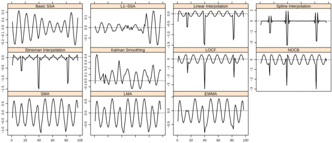
Figures 1-4 show the plots of the errors for different imputation methods for all cases.
215
From these figures we can conclude that the following results satisfy for all cases:
216
1. In the LOCF method, the absolute value of the imputation error increases if the
217
missing value has been placed just after the outlier. However in NOCB method,
218
this is true if the missing value has been placed just before the outlier.
219
2. In interpolation methods (Linear, Spline and Stineman), the absolute values of the
220
imputation error for neighborhoods of the outliers are greater than elsewhere.
221
In case (a), the wave pattern of the imputation error is visible almost for all methods.
222
Also in the L1-SSA method, the imputation error at the end of series is greater than
223
elsewhere.
Location of Missing Value
Error −0.2 −0.1 0.0 0.1 0.2 Basic SSA 0 20 40 60 80 100 −0.1 0.0 0.1 L1−SSA −1.5 −1.0 −0.5 0.0 Linear Interpolation 0 20 40 60 80 100 −2 −1 0 1 Spline Interpolation −1.5 −1.0 −0.5 0.0 Stineman Interpolation −0.1 0.0 0.1 0.2 0.3 0.4 Kalman Smoothing −3 −2 −1 0 LOCF −3 −2 −1 0 NOCB −1.0 −0.5 0.0 0.5 0 20 40 60 80 100 SMA −0.5 0.0 0.5 LMA −0.5 0.0 0 20 40 60 80 100 EWMA
Figure 1: Plots of imputation errors in Sine series (case a).
224
In case (b), the imputation errors show an upward pattern for Kalman smoothing
225
method. Also in Weighted Moving Average methods (SMA, LMA and EWMA), the
226
absolute values of the imputation error for neighbourhoods of the outliers are greater
227
than elsewhere.
Position of Missing Value Error −0.06 −0.04 −0.02 Basic SSA 0 20 40 60 80 100 −0.010 0.000 L1−SSA −0.6 −0.4 −0.2 0.0 Linear Interpolation 0 20 40 60 80 100 −1.0 −0.5 0.0 0.5 Spline Interpolation −0.6 −0.4 −0.2 0.0 Stineman Interpolation −0.05 0.05 0.15 Kalman Smoothing −1.5 −1.0 −0.5 0.0 LOCF −1.5 −1.0 −0.5 0.0 NOCB −0.20 −0.10 0.00 0.05 0 20 40 60 80 100 SMA −0.3 −0.2 −0.1 0.0 LMA −0.4 −0.3 −0.2 −0.1 0.0 0 20 40 60 80 100 EWMA
Figure 2: Plots of imputation errors in Exponential series (case b).
In case (c) similar to case (a), there is wave pattern in imputation errors almost for all
229
methods. Also in theL1-SSA method, the imputation error at the end of series is greater
230
than elsewhere.
Position of Missing Value
Error −1.0 −0.5 0.0 0.5 Basic SSA 0 20 40 60 80 100 −0.6 −0.2 0.0 0.2 0.4 L1−SSA −2 −1 0 Linear Interpolation 0 20 40 60 80 100 −4 −3 −2 −1 0 1 Spline Interpolation −2 −1 0 Stineman Interpolation −5 −4 −3 −2 −1 0 1 Kalman Smoothing −4 −3 −2 −1 0 1 LOCF −5 −4 −3 −2 −1 0 1 NOCB −2 −1 0 1 2 0 20 40 60 80 100 SMA −2 −1 0 1 LMA −1 0 1 0 20 40 60 80 100 EWMA
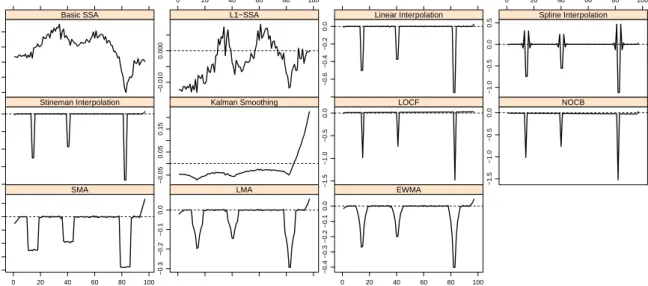
Figure 3: Plots of imputation errors for case c.
231
In case (d), similar to cases (a) and (c), there is wave pattern in imputation errors
232
almost for all methods. Also in this case, the absolute values of the imputation error for
233
neighbourhoods of the outliers are greater than the rest.
Position of Missing Value Error −2 0 2 Basic SSA 0 20 40 60 80 100 −2 −1 0 1 L1−SSA −4 −2 0 Linear Interpolation 0 20 40 60 80 100 −6 −4 −2 0 2 Spline Interpolation −5 −4 −3 −2 −1 0 1 Stineman Interpolation −4 −2 0 2 Kalman Smoothing −5 0 LOCF −8 −6 −4 −2 0 2 NOCB −4 −2 0 2 4 0 20 40 60 80 100 SMA −2 0 2 LMA −3 −2 −1 0 1 2 3 0 20 40 60 80 100 EWMA
Figure 4: Plots of imputation errors for case d.
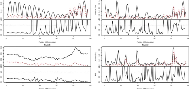
In Figure 5, the plots of absolute errors and RAE for SSA based imputation methods
235
are presented for all cases. Interestingly, it is evident from these figures thatL1-SSA has
236
superiority over Basic SSA for imputation of missing values when there are outliers in
237
time series. The solid and dash lines correspond to basic SSA andL1-SSA, respectively.
238 0.00 0.10 0.20 Case a Index Absolute Error 0 20 40 60 80 100 0.0 0.5 1.0 1.5
Position of Missing Value
RAE 0.00 0.02 0.04 0.06 Case b Index Absolute Error 0 20 40 60 80 100 0.0 0.5 1.0 1.5
Position of Missing Value
RAE 0.0 0.2 0.4 0.6 0.8 1.0 Case c Index Absolute Error 0 20 40 60 80 100 0.0 0.5 1.0 1.5
Position of Missing Value
RAE 0.0 1.0 2.0 3.0 Case d Index Absolute Error 0 20 40 60 80 100 0.0 0.5 1.0 1.5
Position of Missing Value
RAE
Figure 5: Plots of absolute errors and RAE for all cases.
3.4 Real Data
239
In this subsection, the efficiency of imputation methods are compared for imputing of
240
one missing value in real data. To this end, three time series data sets are considered as
241
follows:
1. War series: The U.S. combat deaths in the Vietnam War, monthly from January
243
1966 to December 1971 including 72 observations [33].
244
2. Chickenpox series: Monthly reported number of chickenpox in New York city
245
from January 1931 to June 1972 comprising 498 observations [34].
246
3. Measles series: Number of cases of measles in Baltimore, monthly from January
247
1939 to June 1972 containing 402 observations [35].
248
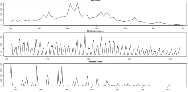
Figure 6 shows the time series plot of these data sets. Here, let us assume that there
249
are two outliers in February and May 1968 in the War series. Also assume that the
250
Chickenpox series includes three outliers in March and April 1949 and March 1953, and
251
that there are three outliers in February 1939, March 1944 and March 1949 in the Measles
252 series. 253 War series Number of deaths 1966 1967 1968 1969 1970 1971 1972 0 500 1000 1500 2000 Chickenpox series Number of cases 1930 1940 1950 1960 1970 0 500 1500 2500 Measles series Number of cases 1940 1945 1950 1955 1960 1965 1970 0 1000 2000 3000 4000
Figure 6: Time series plot of real data.
For reconstructing, L= 21,51,28andr= 7,30,21are used for SSA based imputation
254
in War, Chickenpox and Measles series; respectively. Similar to simulated series, one
255
observation is removed deliberately at different positions to create one missing value.
256
In Table 2, the different imputation methods are compared according to the RRMSE
257
and RMAD criteria. Results indicate that L1-SSA is the best imputation method. It is
258
noteworthy that based on the RRMSE, the next best method is Basic SSA.
Table 2: Comparison of imputation methods for real data.
War series Chickenpox series Measles series
Method RRMSE RMAD RRMSE RMAD RRMSE RMAD
Basic SSA 0.91 0.79 0.98 0.97 0.95 0.77 Linear Inter. 0.86 0.85 0.78 0.79 0.61 0.74 Spline Inter. 0.82 0.77 0.83 0.85 0.83 0.8 Stineman Inter. 0.86 0.84 0.8 0.84 0.63 0.81 Kalman Smoothing 0.81 0.73 0.94 0.97 0.95 0.94 LOCF 0.69 0.68 0.39 0.39 0.35 0.38 NOCB 0.69 0.68 0.39 0.39 0.36 0.39 SMA 0.85 0.83 0.29 0.26 0.28 0.27 LMA 0.88 0.89 0.36 0.33 0.33 0.32 EWMA 0.9 0.91 0.46 0.42 0.39 0.4
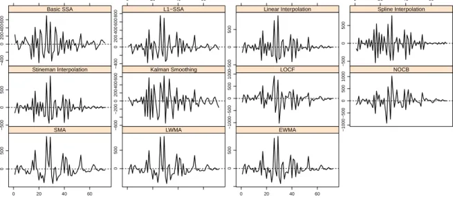
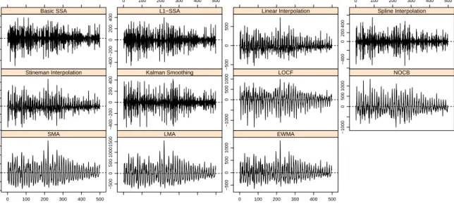
Figures 7-9 depict the plots of imputation errors for different imputation methods. It
260
can be seen that the imputation error increases if the missing value is an outlier.
261
Position of Missing Value
Error −400 0 200 400 600 Basic SSA 0 20 40 60 −400 0 200 400 600 800 L1−SSA −500 0 500 Linear Interpolation 0 20 40 60 −500 0 500 Spline Interpolation −500 0 500 Stineman Interpolation −600 −200 0 200 400 600 Kalman Smoothing −1000 −500 0 500 1000 LOCF −1000 −500 0 500 1000 NOCB 0 500 0 20 40 60 SMA 0 500 LWMA 0 500 0 20 40 60 EWMA
Position of Missing Value Error −400 −200 0 200 400 Basic SSA 0 100 200 300 400 500 −400 −200 0 200 400 L1−SSA −500 0 500 Linear Interpolation 0 100 200 300 400 500 −400 0 200 400 Spline Interpolation −400 0 200 400 600 Stineman Interpolation −400 −200 0 200 400 Kalman Smoothing −1000 0 500 1000 LOCF −1000 0 500 1000 NOCB −1000 0 500 1500 0 100 200 300 400 500 SMA −500 0 500 1000 1500 LMA −500 0 500 1000 0 100 200 300 400 500 EWMA
Figure 8: Plots of imputation errors in Chickenpox series.
Position of Missing Value
Error −500 0 500 Basic SSA 0 100 200 300 400 −500 0 500 1000 L1−SSA −1000 0 1000 Linear Interpolation 0 100 200 300 400 −1500 −500 0 500 Spline Interpolation −1000 0 1000 Stineman Interpolation −500 0 500 Kalman Smoothing −2000 0 1000 2000 LOCF −2000 0 1000 2000 NOCB −1000 0 1000 2000 3000 0 100 200 300 400 SMA −1000 0 1000 2000 LMA −1000 0 1000 2000 0 100 200 300 400 EWMA
Figure 9: Plots of imputation errors in Measles series.
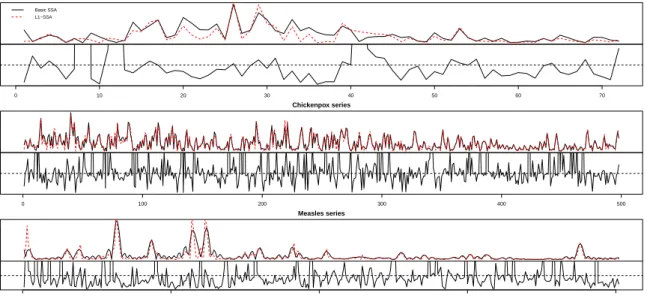
Figure 10 shows the plots of absolute errors and RAE for SSA based imputation
262
methods in real data. From these plots, it can be deduced that almost always, L1-SSA
263
has better performance than Basic SSA.
0 200 500 War series Index Absolute Error Basic SSA L1−SSA 0 10 20 30 40 50 60 70 0.0 1.0 2.0
Position of Missing Value
RAE 0 200 400 Chickenpox series Index Absolute Error 0 100 200 300 400 500 0.0 1.0 2.0
Position of Missing Value
RAE 0 400 Measles series Index Absolute Error 0 100 200 300 400 0.0 1.0 2.0
Position of Missing Value
RAE
Figure 10: Plots of absolute errors and RAE for real data.
4 Conclusion
265In this paper, we proposed a new nonparametric approach for missing value imputation of
266
univariate time series within the SSA framework. In the proposed method, the L1 norm
267
based version of SSA, namely L1-SSA, was applied for imputation of missing values in
268
the presence of outliers.
269
The performance of the new imputation method was compared with many other
estab-270
lished methods such as Interpolation, Kalman Smoothing and Weighted Moving Average
271
with respect to RMSE and MAD criteria using both simulated and real world data.
272
In particular, it was expected that L1-SSA would enable better imputation in
com-273
parison to basic SSA when faced with outliers, because L1 norm is less sensitive than L2
274
norm to the presence of outliers. It is interesting that the comparison of results confirm
275
that almost alwaysL1-SSA outperforms basic SSA.
276
The results obtained in this study also indicates that the SSA based methods (L1
-277
SSA and basic SSA) can provide better imputation in comparison to other methods when
278
faced with time series polluted by outliers. This was proven via both the simulation and
279
application to real data.
280
In terms of future research, the capability of L1-SSA for multiple imputation will be
281
considered. The important issue of selecting the optimal parameters of SSA for
impu-282
tation (L and r) has potential for further exploration, and those interested can begin
283
by considering the research in [21] which presents one approach to the choice of SSA
284
parameters for iterative gap-filling.
285
References
286[1] Chatfield, C. (2000).Time-Series Forecasting. Chapman & Hall/CRC.
[2] Wu. S. F., Chang, C. Y., and Lee, S. J. (2015). Time Series Forecasting with Missing
288
Values. 1st International Conference on Industrial Networks and Intelligent Systems
289
(INISCom), 151–156.
290
[3] Abraham, B. (1981). Missing observations in time series. Communications in
291
Statistics-Theory and Methods,10(16), 1643–1653.
292
[4] Ljung, G. M. (1989). A Note on the Estimation of Missing Values in Time Series.
293
Communications in Statistics-Simulation and Computation, 18(2), 459–465.
294
[5] Harvey, A. C., and Pierse, R. G. (1984). Estimating Missing Observations in Economic
295
Time Series. Journal of the American Statistical Association, 79(385) 125–131.
296
[6] Pourahmadi, M. (1989). Estimation and Interpolation of missing values of a stationary
297
time series. Journal of Time Series Analysis, 10(2), 149–169.
298
[7] Beveridge, S. (1992). Least squares estimation of missing values in time series.
Com-299
munications in Statistics-Theory and Methods, 21(12), 3479–3496.
300
[8] Junger, W. L., de Leon, A. P., and Santos, N. (2003). Missing data imputation in
301
multivariate time series via EM algorithm. Cadernos do IME, 15, 8-–21.
302
[9] Junger, W. L., and de Leon, A. P. (2012). mtsdi: Multivariate time series data
impu-303
tation. R package version 0.3.3, http://CRAN.R-project.org/package=mtsdi.
304
[10] Gomez, V., and Maravall, A. (1994). Estimation, Prediction, and Interpolation for
305
Nonstationary Series with the Kalman Filter. Journal of the American Statistical
As-306
sociation, 89(426), 611–624.
307
[11] Walter, O. Y., Kihoro, J. M., Athiany, K. H. O., and Kibunja, H. W. (2013).
Im-308
putation of incomplete non-stationary seasonal time series data. Mathematical Theory
309
and Modeling, 3(12), 142–-154.
310
[12] Pena, D. (2001). A Course in Time Series Analysis. chap. Outliers, Influential
Ob-311
servations and Missing Data, pp. 136–-170. New York: John Wiley & Sons, Inc.
312
[13] Ansley, C. F., and Kohn, R. (1985). On the estimation of ARIMA models with
313
missing values. Time Series Analysis of Irregularly Observed Data, E. Parzen (ed.),
314
Springer Lecture Notes in Statistics, 25, 9–-37.
315
[14] Jones, R. H. (1980). Maximum likelihood fitting of ARMA models to time series with
316
missing observations. Technometrics, 22, 389–-395.
317
[15] Silva, E. S., and Hassani, H. (2015). On the use of singular spectrum analysis for
fore-318
casting U.S. trade before, during and after the 2008 recession.International Economics,
319
141, 34–49.
320
[16] Hassani, H., Silva, E. S., and Ghodsi, Z. (2017). Optimizing bicoid signal extraction.
321
Mathematical Biosciences, 294, 46–-56.
322
[17] Sanei, S., and Hassani, H., (2016).Singular Spectrum Analysis of Biomedical Signals.
323
Taylor & Francis, CRC Press.
[18] Silva, E. S., Ghodsi, Z., Ghodsi, M., Heravi, S., and Hassani, H. (2017). Cross country
325
relations in European tourist arrivals. Annals of Tourism Research, 63, 151–-168.
326
[19] Hassani, H., Webster, A., Silva, E. S., and Heravi, S. (2015). Forecasting U.S. Tourist
327
arrivals using optimal Singular Spectrum Analysis.Tourism Management,46, 322–335.
328
[20] Schoellhamer, D. H. (2001). Singular spectrum analysis for time series with missing
329
data. Geophysical Research Letters, 28(16), 3187–-3190.
330
[21] Kondrashov, D., and Ghil, M. (2006). Spatio temporal filling of missing points in
331
geophysical data sets. Nonlinear Processes in Geophysics,13, 151–-159.
332
[22] Beckers, J. M., and Rixen, M. (2003). EOF calculations and data filling from
in-333
complete oceanographic datasets.Journal of Atmospheric and Oceanic Technology,20,
334
1839–1856.
335
[23] Hui-zan, W., Rein, Z., Wei, L., Gui-hua, W., and Bao-gang, J. (2008). Improved
336
interpolation method based on singular spectrum analysis iteration and its application
337
to missing data recovery. Applied Mathematics and Mechanics (English Edition), 29,
338
1351-–1361.
339
[24] Golyandina, N., and Osipov, E. (2007). The caterpillar-SSA method for analysis of
340
time series with missing values. Journal of Statistical Planning and Interface, 137(8),
341
2642–-2653.
342
[25] Rodrigues, P. C., and de Carvalho, M. (2013). Spectral modeling of time series with
343
missing data. Applied Mathematical Modelling, 37(7), 4676-–4684.
344
[26] Mahmoudvand, R., and Rodrigues, P. C. (2016). Missing value imputation in time
345
series using singular spectrum analysis. International Journal of Energy and Statistics,
346
4(1), 1650005.
347
[27] Kalantari, M., Yarmohammadi, M., and Hassani, H. (2016). Singular Spectrum
Anal-348
ysis Based on L1-norm. Fluctuation and Noise Letters, 15(1), 1650009.
349
[28] Golyandina, N., Nekrutkin, V., and Zhigljavsky, A. (2001).Analysis of Time Series
350
Structure: SSA and Related Techniques. Chapman & Hall/CRC, Boca Raton.
351
[29] Moritz, S. (2017). imputeTS: Time Series Missing Value Imputation. R package
ver-352
sion 2.5, https://CRAN.R-project.org/package=imputeTS.
353
[30] Korobeynikov, A. (2010). Computation- and space-efficient implementation of SSA.
354
Statistics and Its Interface,3 (3), 257–368.
355
[31] Golyandina, N., and Korobeynikov, A. (2014). Basic Singular Spectrum Analysis and
356
forecasting with R. Computational Statistics and Data Analysis, 71, 934–954.
357
[32] Golyandina, N., Korobeynikov, A., Shlemov, A., and Usevich, K. (2015). Multivariate
358
and 2D Extensions of Singular Spectrum Analysis with the Rssa Package. Journal of
359
Statistical Software,67(2), 1–78. doi:10.18637/jss.v067.i02.
[33] Janowitz, M. F., and Schweizer, B. (1989). Ordinal and Percentile Clustering.
Math-361
ematical Social Sciences,18(2), 135-–186.
362
[34] Hyndman, R. (2017). Monthly reported number of chickenpox, New York
363
city, 1931-1972. Available from Time Series Data Library (TSDL) Web site:
364
https://datamarket.com/data/list/?q=cat:g24%20provider:tsdl.
365
[35] Hyndman, R. (2017). Monthly reported number of cases of measles, Baltimore,
366
Jan. 1939 to June 1972. Available from Time Series Data Library (TSDL) Web site:
367
https://datamarket.com/data/list/?q=cat:g24%20provider:tsdl.