Recognising Guitar Chords in
Real-Time
Michael Goold
Bachelor of Engineering (Software)
Supervised by Dr Du Huynh
This report is submitted as partial fulfilment of the requirements for the Honours Programme of the School of Computer Science and Software Engineering,
The University of Western Australia, 2009
Abstract
Learning to play the guitar is a difficult task, one that requires a great deal of time and patience. In an effort to ease the strain of this process, a Java software package has been designed and developed in order to assist amateur guitarists while they are learning to play their instrument.
The software package achieves this by monitoring the waveform of the music being played, and providing the user with feedback while they play through a song. The player is scored based on how well they play a song, thus making the process less a chore, and more like a game.
There has been a large amount of research devoted to extracting information about music contained in an audio signal, and this paper reviews several such research pa-pers. It later builds on this research by describing the utilisation of these theoretical procedures in a practical application. The algorithms and design choices of this ap-plication are described in detail, with special attention paid to the chord recognition algorithm itself. Finally, an analysis of the effectiveness of this application is provided, with remarks on its accuracy and shortcomings.
Keywords: Guitar, Music, Tuition, Java, Real Time, Spectrum, Chord CR Categories:
Acknowledgements
I would firstly like to thank Dr Du Huynh, for all of her support and guidance through-out this project. Her knowledge of signal processing and the Matlab environment were invaluable. I would also like to thank my family and friends for all of their help, en-couragement and support when I needed it.
Contents
Abstract ii Acknowledgements iii 1 Introduction 1 2 Literature Review 4 2.1 Overview . . . 42.2 Synthesizing Test Notes . . . 6
2.3 Static Vs Dynamic Thresholds . . . 7
2.4 Test Data . . . 7
3 Implementation 8 3.1 Hardware Required . . . 8
3.2 Software Required . . . 8
3.3 Frequency and Pitch . . . 9
3.4 Fourier Transformations . . . 10 3.5 FFT vs DFT . . . 11 3.6 Real-Time Feedback . . . 12 3.7 Matlab Prototype . . . 12 3.7.1 getSpectrum . . . 13 3.7.2 getPeaks . . . 13 3.7.3 checkWave . . . 13 3.8 Guitar Tutor . . . 14 3.8.1 Overview . . . 14 3.8.2 Class Structure . . . 14 3.8.3 XML Song File . . . 17
3.8.4 Reading Microphone Data . . . 19
3.8.5 Calculating the Spectrum . . . 20
3.8.6 Thresholds . . . 21
3.8.7 Playing a Song . . . 22
3.8.8 User Interaction . . . 23
3.8.9 Displaying Results . . . 24
4 Testing and Analysis 28 4.1 Tests Performed . . . 28
4.2 Results . . . 29
4.3 Comparison with Existing Techniques . . . 31
4.4 Viability as Learning Tool . . . 31
4.5 Future Work . . . 32
4.5.1 Recognition Algorithm . . . 32
4.5.2 MIDI Import . . . 32
4.5.3 History . . . 32
5 Conclusion 34 A Appendix A - Peak Detection Algorithm 35 B Appendix B - Original Proposal 37 B.1 Background . . . 37
B.2 Aim and Method . . . 39
B.3 Schedule . . . 40
B.4 Software and Hardware Requirements . . . 40
List of Tables
4.1 One-note tests . . . 28
4.2 Two-note tests . . . 28
4.3 Three-note tests . . . 29
4.4 Four-note tests . . . 29
4.5 Five-note tests. The notes that make up a C Major chord are C3, E3, G3,C4,E4 . . . 30
4.6 Six-note tests. The notes that make up an E Major chord are E2,B2, E3,G#3 ,B3,E4 . . . 31
List of Figures
1.1 Comparison of Digital Guitar (Top), and Standard Analog Guitar
(Bot-tom) . . . 2
1.2 The audio waveform for an E Chord . . . 3
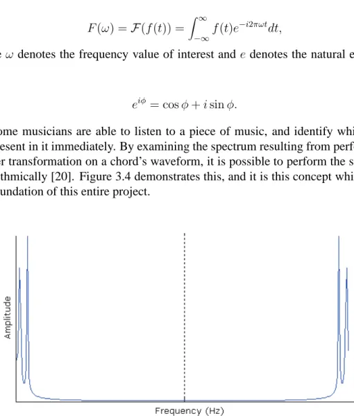
1.3 The frequency spectrum of an E Chord . . . 3
3.1 Acoustic-Electric Guitar, labeled . . . 8
3.2 The notes that make up one octave . . . 9
3.3 Two seperate notes, and the waveform that results from them playing simultaneously . . . 10
3.4 The Fourier transform of the combined waveform shown in Figure 3.3 11 3.5 Labeled screenshot of Guitar Tutor . . . 15
3.6 A UML diagram representation of the classes that make up Guitar Tutor 17 3.7 A data flow diagram illustrating the interaction between classes in Gui-tar Tutor . . . 18
3.8 Generated queue of notes . . . 19
3.9 A waveform before and after Hamming window processing. . . 21
3.10 The spectrum of both a processed and unprocessed waveform. . . 22
3.11 The displayed spectrum for a C chord. . . 26
3.12 The display queue of a song . . . 26
3.13 The results screen for a song . . . 27
B.1 The audio waveform for an E Chord . . . 38
CHAPTER 1
Introduction
While the professional music industry has been blessed with a huge amount of techno-logical innovation, casual musicians have largely been ignored for years. The lack of software available to those who spend their spare time enjoying creating and playing musical instruments is quite startling, considering how quickly the technology behind professional music is advancing. One reason for this is perhaps that instruments such as the guitar cannot be represented digitally.
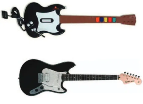
Recently, products such as the Guitar Hero [12] and Rock Band [19] computer game series have attempted to overcome this limitation, by developing basic digital guitars to simulate the experience, but they are far too primitive to be substituted for real guitars when learning the instrument, since there is effectively only one string, and only five frets. Real guitars have 6 strings, and at least 18 frets. It is impractical to expect a digital guitar to be developed, since it would be far more complex than the analog device it is to simulate. Figure 1.1 illustrates the differences between the two.
Some might think that these guitar games help introduce users to the basic tech-niques required to play a guitar, but this is not the case. I have played several of the Guitar Hero games, and have noticed that after having spent time using it, my ability to play a real guitar is temporarily hindered. I must practice with a real guitar for a time in order to ‘unlearn’ the bad habits that Guitar Hero and similar rhythm games promote. The only useful technique being exercised by playing these guitar games is timing. Coordination is nonexistant, since there is no need to place a finger on any specific string. This is true for both hands, since the left hand (the hand the shapes a chord), must only hit a specific button, and the right hand (the hand that strums the strings) must only flick one button up or down, rather than strum a number of strings correctly. Until the digital guitars become more complex and similar to real guitars, they will not be useful as a training aid. However, by the time they do manage to suc-cessfully represent a real guitar, they will be so complex that the price of such a device will probably be just as high as that of a real instrument.
Most music tuition software available today, such as imutus (Interactive Music Tuition Software) [14], Guitar Pro [13] and eMedia Guitar Method [9], allow the user
Figure 1.1: Comparison of Digital Guitar (Top), and Standard Analog Guitar (Bottom)
to play along to some sort of sheet music. However, they do not offer feedback on whether the user is playing the music correctly. They simply provide the user with something to play along with, and judge for themselves how well they are doing. In this way, these software packages do not have much of a ‘fun’ aspect, and are instead only a training aid. One of the most effective methods of teaching someone a new skill is to make it fun. By designing a software package that can train a user to play guitar in a gaming environment, I hope to make it much easier for new guitarists to improve their skill level.
There has been a vast amount of research on automatic transcription and recog-nition of polyphonic music [7, 10, 11, 17, 18, 22]. However, this research has all focused on the problems involved in identifying the fundamental frequency (f0) of a tone, rather than on matching an expected note with one detected. The aim of this project was to develop a software package that would be able to determine whether a detected chord matched an expected chord, and if not, to be able to determine which note(s) were incorrect.
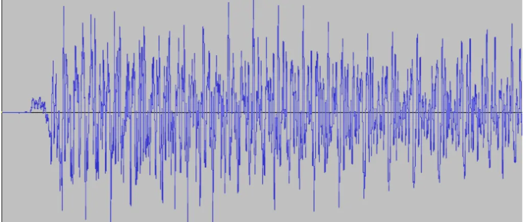
Similar to the approaches presented in Chapter 2, this project has made use of Fourier transformations to extract the music information from an audio waveform. A section of an E Chord’s waveform is shown in Figure 1.2, and the frequency spec-trum of an E Chord is shown in Figure 1.3. The peaks in the specspec-trum correspond to frequencies with high amplitudes. Using this information, it is possible to determine
which notes are the most dominant in an audio sample.
Figure 1.2: The audio waveform for an E Chord
CHAPTER 2
Literature Review
2.1
Overview
In most signal analysis methods, the most important task is the detection of frequen-cies present in the audio signal. The common approach undertaken to achieve this is by analysing the signal in the frequency domain. By performing a Fourier transformation on an audio signal, the frequency spectrum of that signal can be retrieved. All of the articles reviewed in this paper utilise this Fourier transformation in some way. Each paper attempts to extend this basic method in some way so as to increase its effec-tiveness. For instance, Bello et al [7] includes time domain analysis in their approach, while Klapuri [17] simulates the human auditory system, and passes the signal through this model.
Automatic transcription of music is one of the major applications demanding ro-bust musical signal analysis. In the work of Bello et al [7], a method for transcribing polyphonic music is proposed. This approach utilises both the frequency and time domain in its approach. The frequency domain approach used in this method is very similar to other spectrum analysis methods. When applied with the time domain appli-cation however, this method ultimately increases both true and false positives. When analysing the article, it appears that the authors have cut several corners, in an attempt to save time in their experiment. Examples of this include the use of static thresh-olds and MIDI file sound synthesizing. Ultimately however these shortcuts reduce the accuracy of the final results.
Similar to Bello et al’s method, Virtanen and Klapuri [22] utilise the time domain in their approach. The basic frequency domain analysis is extended by using a statistical method called an F-Test to find the spectral peaks. It then tracks these peaks in the time domain. While the research presented in this article seems reasonably effective, there is no mention of actual results. All that is said is that the method is “practically applicable”. The success of this application in practice is therefore questioned, as the author has failed to detail any practical results. Therefore, the authors failed to address the initial aim of their experiment. They were originally trying to accurately separate
each tone present in an audio file, but instead their system “tries to model the human auditory system by connecting trajectories which are close to each other”. This seems to be the complete opposite of separating the notes contained in the audio file.
A basic spectrum analysis method is presented by Raphael [18], which describes an application of the Hidden Markov Model in an attempt to transcribe piano music. The audio signal is segmented into time frames, and each frame is labelled according to observed characteristics. These include elements such as pitch, attack, sustain, and rest. The model must be trained using audio sample / score pairs, and therefore is heavily dependent on the validity of these training pairs. The method has an error rate of around 39%, which is far too high for practical applications. However, the author has stated no attempt was made to analyse the attack portion of each note, which is where most data on the chord is found.
Similar to the well-known “cepstrum” method, Saito et al [10] attempt to anal-yse polyphonic music signals. Instead of taking the inverse Fourier transform of log-arithmically scaled power spectrum with linear scaled frequency, as in the cepstrum method, the specmurt method takes the inverse Fourier transform of linear power spec-trum with logarithmic scaled frequency. The article claims that this method is more effective in determining the notes present in a polyphonic audio signal than the cep-strum method. While this may be the case, the stated average result of 53% success is far too poor for use in a practical application. The authors justify this low success rate by stating that their results are comparable to similar methods, yet are obtained at much faster speeds.
In a major departure from the traditional methods of analysing music signals, Kla-puri [17] presents a novel approach to the task, by implementing a model of the human auditory system and passing the signal through that. The reasoning behind this deci-sion was “that humans are very good at resolving sound mixtures, and therefore it seems natural to employ the same data representation that is available to the human brain”. The method employs several filters that alter the signal in the same way as the human auditory system. While the method attempts to be as faithful as possible to the human auditory system, a Fourier transformation is still required to analyse the spectrum for frequency peaks. The use of an auditory model appears quite effective, outperforming the two methods that the author chose to compare it with. This may be due to the fact that the higher order overtones present in harmonic sounds can better be utilized in an auditory model.
Finally, Every and Szymanski [11] have attempted to simplify the problems asso-ciated with polyphonic music analysis, by separating simultaneous notes in an audio track into individual tracks plus a residual. This method uses a frequency domain anal-ysis to detect tones that are present in the audio file. A frequency dependent threshold is used in this method, as the author states, “peaks for higher frequency harmonics
are too small to be detected by constant thresholds, but are still useful for pitch de-tection, and are perceptually significant”. This article uses very artificial tests, and as such cannot be applied to the real world without further testing. This is because the results presented in the article will be completely different from the results that can be observed using practical data.
While there is no doubt that each of these articles have their own merits, there are several flaws in each that must be addressed. These are detailed below.
2.2
Synthesizing Test Notes
When the time comes to analyse a spectrum and determine which tones it contains, there are several methods one can use. Firstly, one can use an algorithmic method, and try to determine what notes are represented by the frequencies detected. Secondly, one can maintain a database of known sample signals, and compare the spectrum of those signals with the spectrum in question.
If the comparison method is chosen, it must be noted that the extent of the samples database can greatly affect how accurate the results are. Any error in the samples will be amplified by the inherent errors in the processing of the signal and comparison techniques. A real instrument played in a real environment by a real person can sound vastly different from synthesized music. Factors such as the acoustics of the room, human variations in timing, the instruments voice, the quality of the recording device, and even the physical mechanisms that convert human actions to sound, all affect the final sound of the signal. It is impossible to account for all of these factors in synthesis, and so a margin of error is required when comparing a measured signal to a known sample. Synthesizing sounds from MIDI files is a popular option, because it is a quick and easy method of generating a comparison signal. Some methods utilize MIDI files to synthesize test signals for comparison [7, 10].
An alternative to synthesizing test music is to record a variety of real-world sig-nals and test against them. This is a time-consuming and expensive process, since thousands of samples are required to account for the different signals that will be en-countered in practice. For example, Saito et al [10] used a database of 2842 samples from 32 musical instruments. While this is an extensive range of samples, it is still a limiting factor. Signals not catered for in the database are always going to be beyond the capabilities of the system. On the other hand, while a synthesized signal approach will be able to cater for any previously un-encountered signal, its effectiveness will usually be less than an equivalent algorithm that uses pre-recorded music samples.
All of the tests that were conducted in this project were performed with an actual guitar using the application developed throughout the project. As such, the tests are an
accurate representation of the real-world performance of the recognition algorithm.
2.3
Static Vs Dynamic Thresholds
All of the methods presented here require the dominant peaks in the frequency spec-trum to be identified and categorized. The choice of what threshold method to use to determine what constitutes a peak can also affect the accuracy of a signal analysis. The simplest option is to use a static threshold, where frequencies that appear stronger than some pre-determined value are classified as peaks. This was the chosen option in Bello et al [7], However, since the spectral peaks that appear at higher frequencies can often be of a comparable level to the noise that appears at lower frequencies, the static threshold will either discard the high-frequency peaks, or include the low-frequency noise. To counter this problem, Every [11] introduced a frequency-dependent thresh-old, where only the actual peaks are identified as such across the entire spectrum. For similar reasons, dynamic thresholds are used in this project. Rather than frequency-dependent thresholds however, this project uses amplitude-frequency-dependent thresholds. The thresholds for frequencies are calculated based on the amplitudes of nearby frequen-cies, rather than the frequencies themselves.
2.4
Test Data
The data used to test a method can often be used to sway the results in its favour. For example, while Every [11] reports reasonably high results, all of them come from incredibly artificial tests. All of the test sound samples used in the article are of length 2 to 8 seconds, contain between 2 and 7 notes, start at the same time, continue for the same length, and have the same energy. This will never be the case in real-world music, so the validity of the results is reduced. Bello et al [7], on the other hand, tested his method over real music, including pieces by Mozart, Beethoven, Debussy, Joplin, and Ravel. While these real world tests will naturally give lower success rates than artificial tests, the test rsults are a far more accurate representation of the effectiveness of the methods.
CHAPTER 3
Implementation
3.1
Hardware Required
First and foremost, a guitar is necessary. I used a ‘Lyon by Washburn’ Acoustic-Electric guitar, as in Figure 3.1 for all development and testing, however any guitar will suffice. An electric guitar, plugged directly into the microphone port of a com-puter is ideal, since there will be negligible interference. A traditional acoustic or classical guitar can be used, with a microphone placed near the sound chamber to pick up the tones played. While this approach will be adequate, there will be a lot more in-terference because of the microphone. A computer capable of receiving audio input is also necessary, and in my testing I have used both a desktop and a notebook computer. I recommend at least a 1.6 GHz processor, due to the high level of computational effort required.
Figure 3.1: Acoustic-Electric Guitar, labeled
3.2
Software Required
A Java Virtual Machine is required to execute Guitar Tutor. No third-party classes or packages are used, in an effort to maximise portability.
Prototyping and testing were performed using Matlab 7.0 and Audacity. Guitar Tutor was developed using the Eclipse Platform version 3.4.2, on a Windows XP oper-ating system. Testing was also performed using Windows 7, as well as Ubuntu Linux.
3.3
Frequency and Pitch
The frequency and pitch of a sound are similar concepts, and are closely related. Both describe how high a sound is. Frequency is a physical measurement of the number of cycles per second of the sound, and can be measured using scientific instruments. The pitch of a sound is simply a label, describing the relative position of the sound on a music scale. Pitch is used to categorise sounds into groups. The noteA4, above middle C, is generally considered to have a frequency of440Hz. The subscript 4 attached to this note denotes the octave number. There is nothing particularly special about this frequency, but it has been standardised by the ISO to simplify the tuning of orchastras and bands [15]. In fact, in some music circles, the noteA4is tuned to have a different frequency, such as442Hz, to give the music a slightly different mood [8]. All music involved in this project has been tuned withA4 having a frequency440Hz.
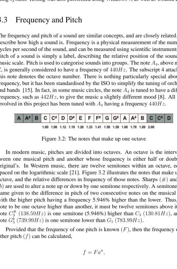
Figure 3.2: The notes that make up one octave
In modern music, pitches are divided into octaves. An octave is the interval be-tween one musical pitch and another whose frequency is either half or double the original’s. In Western music, there are twelve semitones within an octave, equally spaced on the logarithmic scale [21]. Figure 3.2 illustrates the notes that make up one octave, and the relative differences in frequency of those notes. Sharps(#)and Flats
(b)are used to alter a note up or down by one semitone respectively. A semitone is the name given to the difference in pitch of two consecutive notes on the musical scale, with the higher pitch having a frequency 5.946% higher than the lower. Thus, for a note to be one octave higher than another, it must be twelve semitones above it. The note C3# (138.59Hz)is one semitone (5.946%) higher thanC3 (130.81Hz), and the
noteGb
5(739.99Hz)is one semitone lower thanG5 (783.99Hz).
Provided that the frequency of one pitch is known(F), then the frequency of any other pitch(f)can be calculated,
f =F an,
where a is a constant, given by the twelfth root of two, ora= 2121, andnis the number
of semitones between F and f, and can be a negative number. For simplicity, the frequency ofA4(440Hz)is used forF, andnis the number of semitones between f
andA4.
It is a common misconception that there are no such notes asB# orE#, but this
is not the case. Adding a #to a note simply means ‘raised by one semitone’. A B#
note then is simply the same note as aC note, and so too is anE#note the same note
as anF. Indeed, it is acceptable to refer to anEas aD##, or aGbbb, although this is
obviously not a common practice, since there are more convenient ways of describing notes.
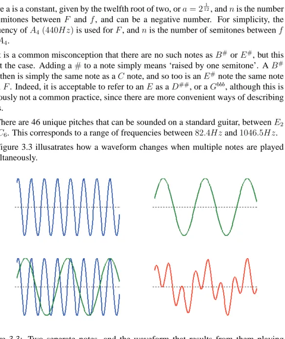
There are 46 unique pitches that can be sounded on a standard guitar, betweenE2
andC6. This corresponds to a range of frequencies between82.4Hz and1046.5Hz. Figure 3.3 illusatrates how a waveform changes when multiple notes are played simultaneously.
Figure 3.3: Two seperate notes, and the waveform that results from them playing simultaneously
3.4
Fourier Transformations
To convert a waveform from its native time domain to the required frequency domain, a Fourier Transformation algorithm must be used. For a continuous function of one variablef(t), the Fourier TransformF(f)is defined as
F(ω) =F(f(t)) =
Z ∞ −∞
f(t)e−i2πωt
dt, (3.2)
where ω denotes the frequency value of interest and edenotes the natural exponent. Thus,
eiφ = cosφ+isinφ.
(3.3)
Some musicians are able to listen to a piece of music, and identify which notes are present in it immediately. By examining the spectrum resulting from performing a fourier transformation on a chord’s waveform, it is possible to perform the same task algorithmically [20]. Figure 3.4 demonstrates this, and it is this concept which forms the foundation of this entire project.
Figure 3.4: The Fourier transform of the combined waveform shown in Figure 3.3
3.5
FFT vs DFT
While the speed of Fast Fourier Transformation algorithms are undeniable when cal-culating the entire spectrum of a waveform, it is innapropriate for this project, since only the 46 frequencies producable on a guitar are of any interest. An FFT algorithm will not only be doing more work than is required, but it will also be less accurate than a Discrete Fourier Transform algorithm, since it returns the total amplitude of discrete
‘blocks’, rather than the amplitude of a specific frequency. For this reason, I have cho-sen to utilise a DFT algorithm for this project. The amplitudes of the 46 frequencies of a guitar will be calculated, using Equation 3.4.
F(ω) = N−1 X k=0 f(tk)e−i2πωtk . (3.4)
By substituting the natural exponent from Equation 3.3, the complex component of this equation can be removed:
F(ω) =
N−1 X
k=0
f(tk) cos(2πωtk) +isin(2πωtk), (3.5) where ω is the frequency whose Fourier amplitude is desired, N is the number of samples in the waveform being analysed, andtk is the time of the sample at position
k.
If the value ofN is known, then it is possible to pre-compute the sine and cosine values to be used in this equation. They can then be stored in arrays, making it a simple task to lookup the relevant value when needed, rather than calculate it. Since this project utilises a sliding window approach, with a constant window size, the value ofN is known and is constant, allowing for a marked improvement in speed over using an FFT approach.
3.6
Real-Time Feedback
Perhaps the requirement that I felt was the most important to be able to satisfy was that the algorithm must execute in real-time. There is no point having to record a sample of music and then analyse the recording, since there are much more elaborate software suites available to do that already. Anything less than execution in real-time would be unacceptable, since the software would not be able to keep up with a player. This would result in either incorrect scoring due to gaps in detection, or an ever-increasing lag throughout a song. Both of these options would be incredibly detrimental to the effectiveness of the software, so there was no option other than real-time feedback.
3.7
Matlab Prototype
A small prototype was developed using Matlab prior to commencement of develop-ment. This prototype served as both a proof-of-concept, as well as a research tool,
used to develop and test the core recognition algorithm to be used in Guitar Tutor. Three M-Files were developed and tested using Matlab:
3.7.1
getSpectrum
getSpectrum()accepts a wav file path as input, and outputs a spectrum approxi-mation of the waveform contained therein.
function [freqs, amps, Fs] = getSpectrum(filepath) [x, Fs, bits] = wavread(filepath); N = 16384; f = 0:Fs/N:(Fs-1/N)/2; h = hamming(length(x),’periodic’); s = h.*x; ft = abs(fft(s,N)); nft = ft(1:length(ft)/2); freqs = f’; amps = nft; end
3.7.2
getPeaks
getPeaks() accepts a wav file path and an integer as input, and outputs an ar-ray containing the frequencies of the specified highest detected amplitudes within the waveform.
function [peakFreqs, peakAmps] = getPeaks(filepath) [f,a,Fs] = getSpectrum(filepath);
aa = peakdet(a,10,500); peakFreqs = aa(:,1)*Fs/16384; peakAmps = aa(:,2);
end
The functionpeakdetcan be found in Appendix A.
3.7.3
checkWave
checkWave()accepts a wav file path, an array of notes to check for, and an error margin as input, and returns an array of the same length as the notes array, containing true or false values representing the presence of each note.
function [ amplitudes, stats, results, normals ] = checkWave( file, N, testNotes, error ) % analyzes the wave in file, checks for notes present
% 1100, so no point caring about whats above the harmonics of that maxHz = 3300;
threshold = 10;
% calculate frequencies of test notes testFreqs = getFreqs(testNotes); % ___GENERATE SPECTRUM___ % % read in the wave file
[signal, rate, bits] = wavread(file);
% generate hamming window and smooth waveform window = hamming(length(signal),’periodic’); processed = window .* signal;
% calculate N-point fourier transform of wave fourier = abs(fft(processed,N));
% retrieve relevant section of transform spectrum = fourier(1:round(maxHz*N/rate));
% calculate mean and standard deviation for normalising stats = [mean(spectrum), std(spectrum)];
% ___TEST FOR EXPECTED NOTES___ %
% for each note expected, determine peak amplitude at that point for i=1:length(testFreqs)
% convert frequency to spectrum index freq = round(testFreqs(i)*N/rate);
% retrieve the peak amplitude of spectrum at desired frequency amplitudes(i) = max(spectrum(freq-error:freq+error));
% determine if this amplitude is above some threshold normalised(i) = amplitudes(i) ./ stats(1);
results(i) = normalised(i) > threshold; end
normals = normalised; end
3.8
Guitar Tutor
3.8.1
Overview
Guitar Tutor is the name of the application developed during this project. A screen shot of Guitar Tutor is shown in Figure 3.5. The following sections describe the application in detail. The Java source code for theControlThreadandSpectrumDFTclasses can be found in Appendix C. The source code for the remaining classes has been omitted from this paper.
3.8.2
Class Structure
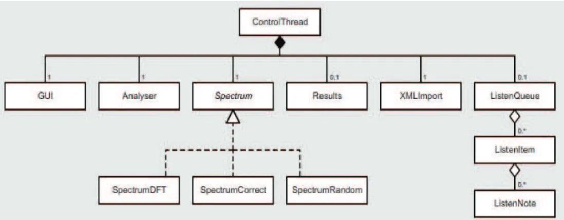
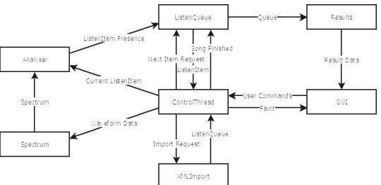
The application developed in this project contains 9 major classes. A UML diagram representation of these classes can be seen in Figure 3.6, and a dataflow diagram in Figure 3.7. The major classes that make up Guitar Tutor are described below.
Figure 3.5: Labeled screenshot of Guitar Tutor
• ControlThread has two main responsibilities. Firstly, it is responsible for extracting the waveform input data from the microphone port, placing it into discrete windows, and passing these windows to the Spectrum implementa-tion in order to retrieve the spectrum of the waveform. In addiimplementa-tion to this,
ControlThread is responsible for playing through a song. It maintains the current beat in the song, as well as the currently expected chord. To read the microphone data,ControlThreadutilises classes and methods contained in the packagejavax.sound.sampled.
• Analyser performs most of functions that deal with note amplitudes. This class maintains a history of each notes’ amplitude, and contains the functions
insertPresence(ListenItem item) and scaleThresholds(). insertPresencedetermines whether the desired notes are present when re-quired, and inserting this presence into the corresponding Note object.
scaleThresholdssets the dynamic threshold values across each note, as-sisting in the determination of their presence.
• Spectrumis an interface containing one method,getAmplitudes(int[] windowData);. This method is required to convert the input waveform
win-dow data to amplitude data. The interface Spectrum has three implementa-tions:
– SpectrumRandom returns a random spectrum every time it is called, many times per beat, and is therefore very innacurate. However, this im-plementation was used extensively while testing Guitar Tutor.
– SpectrumDFT returns the spectrum of the input data, by utilising the Discrete Fourier Transform algorithm as described in Section 3.8.5. On creation, it computes the lookup tables required for the specified array of notes to be detected.
– SpectrumCorrectreturns the spectrum of the currentListenItem.
• Resultsis a representation of the different measures of the player’s success. This class is instantiated with a reference to the ListenQueue that has just been attempted. In its initialisation it steps through eachListenItem, calculating the player’s score.
• ListenQueue houses the data that are required for one complete song. It contains an array ofListenItems, and methods to retrieve these in the correct order.
• ListenItemhouses the data that are required for one chord. In this project, a chord refers to a collection of zero or more notes that must be played simultane-ously. This differs from the traditional definition of a chord, which is a collection of at least three notes.
• Note houses the data that are required for one note. These data include the note’s name, the string and fret number that the note appears on on a guitar, as well as a history of that note’s presence.
• XMLImportconverts XML song files to aListenQueueobject.
• GUIis responsible for presenting the user with all the relevant information they need to use the software. There are two sections to the GUI, the control panel and the canvas panel. The control panel houses all of the buttons, sliders, and combo boxes necessary to control the options relevant to the application, while the canvas panel displays the incoming notes and progress.
Figure 3.6: A UML diagram representation of the classes that make up Guitar Tutor
3.8.3
XML Song File
Being able to easily import new songs to the application was a priority, and so I needed a way to efficiently import song files. It was also important to easily be able to make corrections to a song, in case it contained errors. An XML document structure was chosen to satisfy these requirements.
The XML document contains a number of chordnodes, with aduration at-tribute that defines how many beats this group will last. A second atat-tribute, name, is optional, but can be used to label common chord names.
Figure 3.7: A data flow diagram illustrating the interaction between classes in Guitar Tutor
Eachchordnode has a number of child nodes. These child nodes are thenote
nodes, each representing one of the notes that makes up that chord. Eachnotenode has two attributes,stringandfret, which define which string and fret number the note appears on on the guitar neck. The strings are numbered from thickest to thinnest, with the thickest string being string 0, to the thinnest, which is string 5 (see Figure 3.5).
<song>
<group duration="1">
<note string="1" fret="3" /> </group>
<group duration="1">
<note string="2" fret="2" /> </group>
<group duration="2">
<note string="3" fret="0" /> <note string="4" fret="1" /> </group>
<group duration="4" name="C Major"> <note string="1" fret="3" />
<note string="2" fret="2" /> <note string="3" fret="0" /> <note string="4" fret="1" /> <note string="5" fret="0" />
</group> </song>
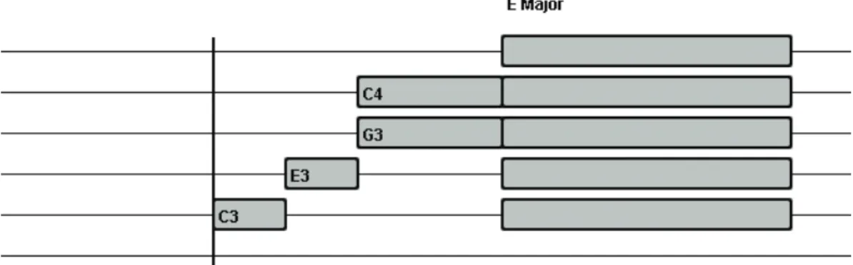
sented to the user graphically. The graphical representation of this song can be seen in Figure 3.8.
Figure 3.8: Generated queue of notes
3.8.4
Reading Microphone Data
Java provides several possible methods of accessing streaming audio data. The pack-agejavax.sound.sampledprovides interfaces and classes for capture, process-ing, and playback of sampled audio data [16].
This project utilises several of the classes within this package:
• Mixerrepresents a physical audio device with one or more lines, in this case, the microphone port.
• DataLineacts as a buffer between a mixer and the rest of the application.
• TargetDataLineis aDataLinefrom which audio data can be read.
• AudioFormatspecifies the values of a range of attributes in an audio stream, such as sample rate, bits per sample, signed or unsigned samples, and the endi-anness of the stream.
On initilisation, the ControlThread specifies the AudioFormatthat audio should be captured in. This project uses a sample rate of44100Hz, 16 bits per sample, one channel, signed data, with little-endian samples.
Next, the desired Mixerobject is selected, which is Java’s representation of an audio device. The availableMixerdevices are listed in a combo box on theGUI.
ControlThreadthen creates a newDataLine object, which acts as a buffer between the Mixer and the rest of the application. ThisDataLineallows data to be
read from the Mixerin the desired format. Finally, thisDataLine is openned on the specifiedMixer.
When running, theControlThreadreads the available bytes off theDataLine
and converts them to integers. It adds these integers to the window data, and gets the amplitudes of the desired notes via Spectrum. ControlThreadthen sends this spectrum data toAnalyserto be added to the running history of amplitudes, for use in later analysis.
Upon clicking theStartbutton, theControlThreadbegins capturing the au-dio from the microphone port. If there are any bytes available to be read from the
TargetDataLine, then these bytes are converted to integers and placed into an array calledwindowData.
This array holds a specified constant amount of audio data, and it is these data whose spectrum is retrieved every loop. The windowData array holds 100ms of data, and is therefore of sizesampleRate/10 = 4410. This size was chosen in order to be able to contain a large enough number of complete waveforms of a chord to get an accurate spectrum, while still being small enough that short chords can be detected. The spectrum of windowData is retrieved by SpectrumDFT and passed to
Analyserto be added to a running history of amplitude data.
3.8.5
Calculating the Spectrum
The spectrum is calculated by performing the Discrete Fourier Transform function as defined in Equation 3.5 on the window data. Unfortunately, the window data are not a continuous function. The abrupt ends of the waveform will cause spectral leakage in the returned spectrum. This is very undesirable in this project, since fine detail of the spectrum is required to distinguish notes that are close together.
In order to compensate for these abrupt ends of the waveform, it is pre-processed using a Hamming window,
W(n) = 0.54−0.46 cos
2πn
N −1
, (3.6)
whereN is the width of the discrete-time window function, and nis an integer, with values0≤n < N
The waveform’s hard edges are minimised, and the resulting spectrum will be less affected by spectral leakage. A demonstration of this processing can be seen in Fig-ures 3.9 and 3.10. While the amplitudes of peaks in the processed waveform are re-duced by a factor of about 2, there is a reduction in noise by a factor of about 10. This
is a dramatic improvement in spectrum quality. There is even greater improvement in the purity of the peaks, which are much sharper in the processed waveform’s spectrum.
Figure 3.9: A waveform before and after Hamming window processing.
Due to the fact that notes at the low end of the spectrum have very similar frequen-cies, when determining the amplitude of a note, its first two harmonics are taken into account.
The values of the hamming window and the lookup tables for the sine and cosine values of Equation 3.5 are calculated once, during the initialisation ofSpectrumDFT. Two 2-dimensional arrays of sizenumNotes∗windowSizeare created to store these values.
The code to calculate these values is as follows:
for(int i=0;i<windowSize;i++) { // calculate time at this index
time[i] = i/((float)windowSize-1)*duration; for(int j=0;j<om.length;j++) {
// calculate the r/i values of exp(-i*2*pi*om*t) at this index tableReal[j][i] = Math.cos(2*Math.PI*omHarmonics[j]*time[i]); tableImag[j][i] = -Math.sin(2*Math.PI*omHarmonics[j]*time[i]); }
// calculate the hamming window value at this index
hammingValues[i] = 0.54 - 0.46*Math.cos(2*Math.PI*i)/(windowSize-1); }
3.8.6
Thresholds
Through experimentation, it was found that there was a discrepancy between the am-plitudes of the low and high pitch notes. The amam-plitudes of low-pitched notes were never as high as those of higher pitched notes. A threshold dependent on the frequency of the note was required in order to compensate for this.
Figure 3.10: The spectrum of both a processed and unprocessed waveform.
t(f) = 1000000(15−500f), (3.7) wheret(f)is the threshold at frequencyf.
3.8.7
Playing a Song
If a song is playing, thenControlThreaddetermines the currently expected chord, based on the beat the stream is up to. Analyser calculates the presence of this current chord, and adds this presence to a running history of presence data, to be used in the marking of the user’s attempt at playing the song.
Finally, the ControlThread checks to see whether the song is completed. If not, it increments the current chord and repeats. If the song is completed, then the
3.8.8
User Interaction
To interact with the user, a graphical user interface (GUI) was designed. The interface consists of two sections, the Control Panel and the Canvas.
The Control Panel houses all of the buttons, sliders and combo boxes that the user can interact with. These controls are listed below.
• Start / Stop Button. This button tells the application to begin capturing and analysing audio. It acts as a toggle, changing between Start and Stop on each click.
• Available Devices ComboBox. This combo box allows the user to select the audio capture device to use in the application. It is populated with all of the audio devices available to Java.
• BPM Slider / Textbox. These controls allow the user to change the speed at which songs are played. This will change the difficulty of the song, as having a lower BPM value will give the player longer to change their fingering position.
• Load Song ComboBox / Button. These controls allow the user to select a song from the available songs list, and then load its contents into theListenQueue.
• Clear Song. This button clears the currentListenQueue.
• Display Option ComboBox. This ComboBox allows the user to change the way note information is displayed to them in the display queue.
While a song is being played, many of the controls become inactive, to prevent the user from changing settings that are unnecessary during a song. The Available Devices ComboBox, the Load Song Button and ComboBox, and the Clear Song Button are all disabled until the song is stopped. During a song, the user is able to change its BPM, as well as the display option.
Below the Control Panel is the Canvas, which displays all the information about the input waveform, as well as the incoming notes of the current song. There are two distinct sets of information that is presented in the Canvas, the Spectrum, and the Display Queue.
The Spectrum is a graphical representation of the current waveform’s frequency spectrum. There are 45 distinct bars that extend upwards from the bottom of the Can-vas, each representing the amplitude of a single note on a guitar. The horizontal grey lines across each bar represent the threshold currently applied to the bar’s note. An
image of the spectrum can be seen in Figure 3.11, where the horizontal axis denotes the discrete frequency values and the height of each bar denotes the amplitude.
The Display Queue is a graphical representation of the current ListenQueue
object, and is only present when aListenQueueobject is initialised. The six hori-zontal lines across the Canvas each represent one string on a guitar, with the thinnest string at the top. The thick vertical line crossing these string lines is called the ‘Strike Line’, and represents the current progress of the song.
Scrolling across the Canvas from the right-hand side are a number of grey rect-angles, each representing a single note. These notes are centred on the ‘string’ that the note can be found on. Depending on the selected display option, the notes can be labeled with either the fret number they can be found on on the note’s string, or the note’s name and octave. Chords are represented by a number of notes aligned verti-cally. If the chord has a common name, it will appear above the group of notes. The width of these notes represents the duration it should be sounded for. The note icons scroll to the left at a rate of 7500 pixels per minute, or 125 pixels per second. This means that at 80 beats per minute, there are 94 pixels per beat, and at 180 beats per minute, there are 41 pixels per beat.
As notes pass the Strike Line, the user is instantly provided with feedback on the presence (or absence) of each note over time. The portion of the note that extends be-yond the Strike Line will be coloured, either red, or a hue somewhere between yellow and green. Times where the note was not detected at all (i.e. its bar in the spectrum did not protrude above the threshold line) are represented with the colour red. If the note was detected, then the colour represents how clear the note was among its neighbours. Yellow indicates that the note was only marginally stronger than the threshold, and green indicates that it was much stronger. An image of the display queue can be seen in Figure 3.12.
3.8.9
Displaying Results
Upon completing a song, the user is presented with a summary of the results of their attempt. These results include:
• Summary of song. A summary of the song’s details is presented to the user. This summary includes the number of notes and chords in the song, as well as a rating out of five representing the song’s difficulty level.
• Number of notes played correctly. A note is judged as being correct if it was detected as present for more than 75% of its duration.
• Number of chords played correctly. A chord is judged as being correct if at least 75% of its notes are correct.
• Total score. The total score of a song is calculated as the number of correct chords divided by the total number of chords.
Figure 3.11: The displayed spectrum for a C chord.
CHAPTER 4
Testing and Analysis
This project is centered around the chord detection algorithm, and as such this algo-rithm needed to be tested thoroughly for accuracy.
4.1
Tests Performed
6 song files were created to test the detection algorithm. Each song consists of a number of repetitions of the same 1 to 6 note chord. Each chord in these files is labelled with a description of the notes to actually be played at that point in the song. Each chord and input combination is repeated 3 times, and each chord lasts one beat. The songs were played at 80 beats per minute. Listed in Tables 4.1 - 4.6 are the the tests performed, and their results. The last three columns of each table show the results of the three repeated experiments for each test.
Expected Note Played Note Expected Result System Pass / Fail
C3
– Fail Pass Pass Pass
E3 Fail Pass Pass Pass
C3 Pass Pass Pass Pass Table 4.1: One-note tests
Expected Note Played Expected Result System Pass / Fail
C3 /E3
– / – Fail Pass Pass Pass
D3/ – Fail Pass Pass Pass
D3/F3 Fail Pass Pass Pass
C3/F3 Fail Pass Pass Pass
C3/ – Fail Pass Pass Pass
C3/E3 Pass Pass Pass Pass Table 4.2: Two-note tests
Expected Note Played Expected Result System Pass / Fail
C3 /E3 /G3
– / – / – Fail Pass Pass Pass
D3/ – / – Fail Pass Pass Pass
D3/F3/ – Fail Pass Pass Pass
D3/F3/A3 Fail Pass Pass Pass
D3/F3/G3 Fail Pass Pass Pass
D3/E3/G3 Fail Pass Pass Pass
C3/ – / – Fail Pass Pass Pass
C3/E3/ – Fail Pass Pass Pass
C3/E3/G3 Pass Pass Pass Pass Table 4.3: Three-note tests
Expected Note Played Expected Result System Pass / Fail
C3/E3/G3/C4
– / – / – / – Fail Pass Pass Pass
D3/ – / – / – Fail Pass Pass Pass
D3/F3/ – / – Fail Pass Pass Pass
D3/F3/A3/ – Fail Pass Pass Pass
D3/F3/A3/D4 Fail Pass Pass Pass
D3/F3/A3/C4 Fail Pass Pass Pass
D3/F3/G3/C4 Fail Pass Pass Pass
D3/E3/G3/C4 Fail Pass Pass Fail
C3/ – / – / – Fail Pass Pass Pass
C3/E3/ – / – Fail Pass Pass Pass
C3/E3/G3/ – Fail Pass Fail Pass
C3/E3/G3/C4 Pass Pass Pass Pass Table 4.4: Four-note tests
4.2
Results
The results of these tests demonstrate the robustness of the implemented chord de-tection algorithm. Chords containing one to four notes were detected successfully on most occasions, having failed only two tests of 90 in the tests performed on this range of notes. As expected, the 5 and 6 note tests began returning false positive results. This is easily attributed to the harmonics of low notes being strong enough to be detected as those same notes from a higher octave. Interestingly, the 6 note tests as seen in Table 4.6 were a lot less successful than anticipated. When the algorithm is listening for an E major chord, it returns a false positive when onlyE2andB2 are played. This is because the notesE3,B3andE4 are falsely detected among the harmonics of these two supplied notes. The algorithm then is satisfied that 5 of the 6 desired notes are
Expected Note Played Expected Result System Pass / Fail
C Major
– / – / – / – / – Fail Pass Pass Pass
D3/ – / – / – / – Fail Pass Pass Pass
D3/F3/ – / – / – Fail Pass Pass Pass
D3/F3/A3/ – / – Fail Pass Pass Pass
D3/F3/A3/D4/ – Fail Pass Pass Pass
D3/F3/A3/D4/F4 Fail Pass Pass Pass
D3/F3/A3/D4/E4 Fail Pass Pass Pass
D3/F3/A3/C4/E4 Fail Pass Pass Pass
D3/F3/G3/C4/E4 Fail Pass Pass Pass
D3/E3/G3/C4/E4 Fail Pass Pass Pass
C3/ – / – / – / – Fail Pass Pass Pass
C3/E3/ – / – / – Fail Pass Pass Pass
C3/E3/G3/ – / – Fail Fail Pass Pass
C3/E3/G3/C4/ – Fail Pass Fail Fail
C3/E3/G3/C4/E4 Pass Pass Pass Pass Table 4.5: Five-note tests. The notes that make up a C Major chord areC3, E3, G3,
C4,E4
present, and it forgives the non-presence of G#3, and returns a positive result for the
chord. This was very unexpected, since only two of six notes were actually sounded. In the application, it was assumed that instead of false positives in a six note chord, that there would instead be a number of false negatives due to the high level of noise present when six strings are sounded together.
There were no false negatives returned anywhere in the entire testing process. This is a fantastic result, since false negatives would be a major detriment to a player’s enjoyment of the software, being seen as unfair. While false positives are still errors in detection, they are much less likely to have an effect on a players enjoyment of the software.
The fact that the chord recognition algorithm does not check for additional notes almost certainly affects the results obtained. The algorithm would become much less generous with positive results when checking against extraneous notes in a chord. However, due to the nature of the scoring system used in this project, where each expected note is either detected or not, there was no intuitive way to penalise the player for sounding additional notes. The presence of the expected notes could certainly not be altered due to additional notes, since the user could be told that they did not play the correct note. The extraneous note information must therefore be presented in some other way, which is why it has not been implemented yet.
Exp. Note Played Exp. Result System Pass / Fail
E Major
– / – / – / – / – / – Fail Pass Pass Pass
F2/ – / – / – / – / – Fail Pass Pass Pass
F2/C3/ – / – / – / – Fail Pass Pass Pass
F2/C3/F3/ – / – / – Fail Pass Pass Pass
F2/C3/F3/A#3 / – / – Fail Pass Pass Pass F2/C3/F3/A#3 /C4/ – Fail Pass Pass Pass F2/C3/F3/A3#/C4/F4 Fail Pass Pass Pass F2/C3/F3/A3#/C4/E4 Fail Pass Pass Pass F2/C2/F3/A3#/B4/E4 Fail Pass Pass Fail F2/C2/F3/G3#/B4/E4 Fail Pass Pass Pass F2/C2/E3/G3#/B4/E4 Fail Fail Pass Pass F2/B2/E3/G3#/B3/E4 Fail Pass Pass Pass E2/ – / – / – / – / – Fail Pass Pass Pass
E2/B2/ – / – / – / – Fail Pass Fail Pass
E2/B2/E3/ – / – / – Fail Fail Fail Pass
E2/B2/E3/G#3/ – / – Fail Fail Fail Fail E2/B2/E3/G#3/B3/ – Fail Fail Fail Fail E2/B2/E3/G3#/B3/E4 Pass Pass Pass Pass
Table 4.6: Six-note tests. The notes that make up an E Major chord are E2, B2, E3,
G#3,B3,E4
4.3
Comparison with Existing Techniques
It is not possible to make a direct comparison of the results of the recognition algo-rithm developed in this project and the results of the papers mentioned in Chapter 2. This is because the focus of this project is fundamentally different from these papers algorithms. All of the papers mentioned in Chapter 2 are focused on extracting data from a sound sample with no information about the sample. This project however, requires knowledge of the notes expected, as well as when they are expected. This greatly simplifies the process of identifying the presence of the desired notes.
4.4
Viability as Learning Tool
The results of the tests performed suggest that this application will certainly be able to assist amateur guitarists in learning to play the guitar. There are still areas where a software package will not be able to replace an actual tutor, such as left hand
fin-ger technique. However, the feedback of this application makes it a more effective practicing tool than a purely offline experience.
4.5
Future Work
There were several features planned for inclusion in Guitar Tutor, that were unable to be implemented due to time constraints. These are detailed below.
4.5.1
Recognition Algorithm
One improvement to the chord recognition algorithm that I would like to see is the ability to detect unexpected notes, and penalise the user for playing them. The current version of Guitar Tutor only checks to see if the expected notes are present. It does not guarantee that there are no additional notes in the chord. Besides this, I am certain that vast improvements to the detection algorithm are possible, if given enough time to find.
4.5.2
MIDI Import
A further improvement to Guitar Tutor would be adding the ability to import a guitar track from a MIDI file. This would eliminate the necessity to write XML song files manually, and would greatly increase the available number of song titles.
In addition to the importing of MIDI song data, being able to use a MIDI syn-thesizer to generate musical notes would allow Guitar Tutor to play a sample of any song to the user upon request. This would give the user a greater idea of what they are attempting to play, and also allow for the playing of duets and other multi-instrument songs.
During development, Java’s implementation of a MIDI engine was examined, and it was decided that these features would take too long to properly implement. Since they were not key requirements in the project, they were left out for future work.
4.5.3
History
A further significant improvement possible is the ability to track user’s progress through-out their use of the software. Having a user profile would allow the application to maintain a history of that user’s attempts, as well as the score they achieved on each
play through. Tracking their progress as time passes would then be possible, allowing them to set performance goals and monitor their improvement.
CHAPTER 5
Conclusion
As demonstrated in this paper and the accompanying software package developed, it is possible to recognise guitar chords in real time. This will be a major benefit to amateur guitarists, as the process of learning to play a guitar can be more easily digitised. Playing a guitar can now be self-taught in the comfort of your own home, at a time that is convenient to the student. This is not the say that there is no need for a tutor at all anymore, simply that they no longer need to be present in order to learn a new song, and provide feedback to the player on sections of the song that they are not quite able to play. Instead, the player will be able to concentrate on learning the song, rather than spending time on deciding if what they are playing is actually correct.
The software package that has been designed and developed provides all of the functionality that is required in order to automate the process of learning to play a guitar. This software package is very basic, with several useful features absent. The core recognition algorithm performs its task well, having demonstrated that it is able to detect chords successfully most of the time. When it does return an incorrect result, it has always been a false positive rather than a false negative. This allows the software package to give the player the ‘benefit of the doubt’ when faced with a difficult chord. This is what a good tutor would do, since they are always aiming to encourage their pupils, rather than demoralise them.
APPENDIX A
Appendix A - Peak Detection Algorithm
function [maxtab, mintab]=peakdet2(v, delta, maxX, x) %PEAKDET Detect peaks in a vector
% [MAXTAB, MINTAB] = PEAKDET(V, DELTA) finds the local % maxima and minima ("peaks") in the vector V.
% MAXTAB and MINTAB consists of two columns. Column 1 % contains indices in V, and column 2 the found values. %
% With [MAXTAB, MINTAB] = PEAKDET(V, DELTA, X) the indices % in MAXTAB and MINTAB are replaced with the corresponding
% X-values.
%
% A point is considered a maximum peak if it has the maximal % value, and was preceded (to the left) by a value lower by
% DELTA.
% Eli Billauer, 3.4.05 (Explicitly not copyrighted).
% This function is released to the public domain; Any use is allowed. maxtab = [];
mintab = [];
v = v(:); % Just in case this wasn’t a proper vector if nargin < 3 maxX = length(v); end if nargin < 4 x = (1:length(v))’; else x = x(:); if length(v)˜= length(x)
error(’Input vectors v and x must have same length’); end
end
if (length(delta(:)))>1
error(’Input argument DELTA must be a scalar’); end
if delta <= 0
error(’Input argument DELTA must be positive’); end
mn = Inf; mx = -Inf; mnpos = NaN; mxpos = NaN;
lookformax = 1; for i=1:maxX
this = v(i);
if this > mx, mx = this; mxpos = x(i); end if this < mn, mn = this; mnpos = x(i); end if lookformax
if this < mx-delta
maxtab = [maxtab ; mxpos mx]; mn = this; mnpos = x(i); lookformax = 0;
end else
if this > mn+delta
mintab = [mintab ; mnpos mn]; mx = this; mxpos = x(i); lookformax = 1;
end end end
APPENDIX B
Appendix B - Original Proposal
B.1
Background
While the professional music industry has been blessed with huge amounts of tech-nological innovation, casual musicians have largely been ignored for years. The lack of software available to those who spend their spare time enjoying creating and play-ing musical instruments is quite startlplay-ing, considerplay-ing how quickly professional music technology is advancing. Perhaps the reason for this is that instruments such as the guitar cannot be represented digitally.
Recently. products such as the Guitar Hero [4] computer game series have devel-oped basic digital guitars to simulate the experience, but they are far too primitive to be used as training aids for a real guitar, since there is effectively only one “string”, and only 5 “frets”. Real guitars, on the other hand, have 6 strings, and at least 18 frets. It is impractical to expect a digital guitar to be developed, since it would be far more complex than the analog device it is to simulate.
There has been a vast amount of research on automatic transcription of polyphonic music [1, 3]. However, this research has all been focusing on the problem of iden-tifying the fundamental frequency (f0) of each note. This project does not require knowledge of f0, since the octave a chord was played at is irrelevant.
Most music tuition software available today, such as imutus (Interactive Music Tuition Software) [6], Guitar Pro [5] and eMedia Guitar Method [2], allow the user to play along to some sort of sheet music. However, they do not offers feedback on whether the user is playing the music correctly. This project aims to rectify this lack of feedback by developing an algorithm to judge the accuracy of a played chord. This can then be extended to a software package to aid in the training of guitarists.
Figure B.1: The audio waveform for an E Chord
B.2
Aim and Method
1. Recognition Algorithm. This project aims to develop an algorithm to determine whether a chord was played correctly in real-time. The algorithm will utilize Fourier Transforms to convert the audio wave into its frequency components. For example, the audio wave in Figure B.1 represents to first 0.5 seconds of an E chord. The frequency spectrum in Figure B.2 is the fourier transform of that E chord. The peaks in Figure B.2 correspond to the frequencies of highest amplitude. Since the algorithm will be given the expected chord as input, it will be able to determine how far from the expected chord the users attempt was.
2. Algorithm Accuracy. 100% accuracy would be desirable, but probably un-achievable, due to noise and improper tuning of the user’s guitar. This project aims to satisfy the following table:
Notes in chord Success Rate
1 95% 2 90% 3 85% 4 80% 5 75% 6 70%
3. Training Software Design. A software package will be designed to facilitate the learning of new songs, by calculating the percentage of notes / chords success-fully played in time to the music expected.
4. Further Tasks. If time permits, the software package itself will be developed and tested. Furthermore, if possible, the algorithms input of expected chord will be removed, allowing the algorithm to interpret any chord.
B.3
Schedule
Month Duration Task
March 1 Week Research / evaluate pitch recognition algorithms March 2 Weeks Research recognition of chords
March 1 Week Compare suitability of paradigms / languages
April 2 Weeks Design terminal application to provide proof of concept April 1 Week Develop shell application
April 5 Weeks Design extended application May 1 Month Develop extended application
June 6 Weeks Test and modify the application as needed July 2 Months Write disseration
September 2 Weeks Edit dissertation September 2 Weeks Write seminar
October 1 Week Present seminar October 1 Week Create Poster
B.4
Software and Hardware Requirements
1. Personal Computer / Laptop with Sound Card
2. Electric Guitar
3. 6.35mm mono audio cable (2 metre length)
4. 6.35mm to 3.5mm mono audio converter
References
[1] J. P. Bello, L. Daudet, and M. B. Sandler. Automatic transcription of piano mu-sic using frequency and time-domain information. IEEE Transactions on Audio,
Speech, and Language Processing, 14(6):2242–2251, November 2006.
[2] eMedia Guitar Method. http://www.emediamusic.com/gm1.html.
[3] Shoichiro Saito et al. Specmurt analysis of polyphonic music signals. IEEE
Trans-actions on Audio, Speech, and Language Processing, 16(3):639–650, March 2008.
[4] Guitar Hero. http://hub.guitarhero.com.
[5] Guitar Pro Music Tablature Software.http://guitar-pro.com/en/index.php.
APPENDIX C
Appendix C - Java Source Code
package tutor;
import java.io.FileNotFoundException; import javax.sound.sampled.*;
public class ControlThread extends Thread { // components
protected GUI myGUI; protected XMLImport myXML; protected Spectrum mySpectrum; public Analyser myAnalyser; protected ListenQueue myQueue;
// mixer (audio devices) names available protected String[] availableMixers; protected int selectedMixer; // samples per second
public final static int sampleRate = 44100; // amount of samples in one analysis
public final static int windowSize = sampleRate/7; // names of notes to process
// NOTE: the length of this array and the index of "A4" within it // are used to calculate the frequencies of these notes,
// not the names themselves
public final static String[] noteNames = {
"E2","F2","F#2","G2","G#2","A2","A#2","B2","C3","C#3","D3","D#3", "E3","F3","F#3","G3","G#3","A3","A#3","B3","C4","C#4","D4","D#4", "E4","F4","F#4","G4","G#4","A4","A#4","B4","C5","C#5","D5","D#5", "E5","F5","F#5","G5","G#5","A5","A#5","B5","C6"
};
// the indices within this array of the open strings (E2, A2, D3, B3, E4) public final static int[] openStringIndices = {0, 5, 10, 15, 19, 24}; // number of notes being "listened for"
public final static int numNotes = noteNames.length; // frequencies of these notes
public final static double[] noteFreqs = getFrequencies(noteNames); // number of harmonics to include in the analysis
public int numHarmonics;
public DrawOption drawOption = DrawOption.FRET_NUM; // defaults
public static int beatsPerMinute = 100; public static int pixelsPerBeat = 60; // currently capturing audio?
public boolean capturing = false;
// buffer to hold the bytes coming off the stream private byte[] byteBuffer;
// window data to be analysed private int[] windowData; // current listen item
public ListenItem currentItem;
// currently playing a song from file? protected boolean playingSong;
// data line to read data from private TargetDataLine dataLine; // current beat
protected double currentBeat; // data stream will be bigEndian? private boolean bigEndian; protected double[] latestResults; protected double[][] resultSet; // create a new controller
public static void main(String args[]) { new ControlThread();
} /**
* Create a new ControlThread */
public ControlThread() {
// get the list of available mixers availableMixers = getMixers();
// select one by default. 3 works on my home computer selectedMixer = 3;
//
numHarmonics = 2;
// playingSong determines whether to listen for notes, // or just sandbox mode
playingSong = false; initialiseCapture();
// initialise an XML importer myXML = new XMLImport(); // initialise an analyser
//mySpectrum = new SpectrumCorrect(this); mySpectrum = new SpectrumDFT(this, noteFreqs); // initialise a result set
myAnalyser = new Analyser(this, 500, 5); // initialise a GUI
myGUI = new GUI(this, 640, 480); this.start();
} /**
* Load a song from xml file
* @param filename The path of the song to load */
public void loadSong(String filename) { System.out.println("Loading " + filename); try {
// get the queue of items to listen for myQueue = myXML.importDocument(filename); beatsPerMinute = myQueue.bpm; myGUI.sldSpeed.setValue(beatsPerMinute); myGUI.txtSpeed.setText("" +beatsPerMinute); currentBeat = 0; currentItem = myQueue.getFirstItem(); playingSong = true; myGUI.repaint(); } catch(Exception e) {
System.out.println("Error loading file. Check file exists and retry"); }
myGUI.repaint(); }
/**
* Clear current song *
*/
public void clearSong() {
System.out.println("Song cleared"); myQueue.clearQueue();
playingSong = false; }
/**
* Gets a list of available mixers.
* This list is used to populate the mixer combobox in the GUI * @return an array of available mixer names
*/
private String[] getMixers() {
Mixer.Info[] mixerInfo = AudioSystem.getMixerInfo(); String[] mixers = new String[mixerInfo.length]; for (int i = 0; i < mixerInfo.length; i++) {
mixers[i] = mixerInfo[i].getName(); }
} /**
* Selects a mixer to be used to capture audio * @param mixerID the index of the chosen mixer */
public void selectMixer(int mixerID) { selectedMixer = mixerID;
}
// initialise the capture of audio private void initialiseCapture() {
try {
// construct an AudioFormat to attempt to capure audio in AudioFormat audioFormat = new AudioFormat(
sampleRate, 16, 1, true, false); // specify the desired data line
DataLine.Info dataLineInfo = new DataLine.Info( TargetDataLine.class, audioFormat);
// select the desired audio mixer Mixer mixer = AudioSystem.getMixer(
AudioSystem.getMixerInfo()[selectedMixer]);
// get a data line (can be read from) on the selected mixer dataLine = (TargetDataLine) mixer.getLine(dataLineInfo); // open the data line
dataLine.open(audioFormat); // initialise the buffers
byteBuffer = new byte[windowSize*2]; windowData = new int[windowSize]; } catch(LineUnavailableException e) { System.out.println(e.getMessage()); } catch(Exception e) { System.out.println(e.getMessage()); } } /**
* begin the capture and analysis of audio */
public void startCapture() { dataLine.flush();
dataLine.start(); capturing = true; }
/**
* end the capture and analysis of audio */
public void stopCapture() { dataLine.stop();
capturing = false; }
public void run() { try {
while(true) {
// loop while capturing is true if(capturing) {
// determine how many bytes are available to be read int available = dataLine.available();
if(available > 0) {
// read as many bytes as possible into the byteBuffer, // up to the size of the buffer
int bytesRead = dataLine.read(
byteBuffer, 0, Math.min(available, byteBuffer.length)); //currentFrame += bytesRead;
currentBeat += (double)bytesRead/sampleRate/120*beatsPerMinute; int intsRead = bytesRead / 2;
// shift windowData left to make room for the new data for(int i=0;i<windowData.length - intsRead; i++) {
windowData[i] = windowData[i+intsRead]; }
// append the new data to the end of windowData for(int i=0;i<intsRead;i++) {
int newInt = bigEndian ?
(byteBuffer[i*2] << 8 | byteBuffer[i*2+1]) : (byteBuffer[i*2+1] << 8 | byteBuffer[i*2]); windowData[i+windowData.length-intsRead] = newInt; }
// add detected notes to results
myAnalyser.insertAmplitudes(mySpectrum.getAmplitudes(windowData)); myAnalyser.scaleThresholds();
// if a song is playing from file, then listen for its notes if(playingSong) {
// determine whether expected notes are present myAnalyser.insertPresence(currentItem);
// move on to the next item when needed
if(currentBeat >= currentItem.startBeat+currentItem.duration) { // if there are more items to listen for
if(!myQueue.queueDepleted()) { currentItem = myQueue.getNextItem(); } else { System.out.println("Song complete"); // songs complete capturing = false;
Results myResults = new Results(myQueue); clearSong();
myGUI.txtResults.setText(myResults.toString()); myGUI.resultsPanel.setVisible(true);
Figure


Outline
Related documents