Engineering Change Request:
Station Voltage Buffers for Transients Position Localization
and Follow-up
Jean-Pierre Macquart, Cath Trott and the Transients SWG June 13, 2014
Summary of Scientific Justification
In many instances, the scientific payoff from the detection of an astrophysical event is only realised once it is localised. Event localization is paramount in the characterisation of one-off transient events, where the position is necessary to associate the event with a specific object or host galaxy. This is necessary to determine its distance and thus energetics, and, through multi-wavelength followup, its origin. The determination of burst positions has historically been central to the transients field, a key example being the use of accurate positions from the BeppoSAX satellite to resolve the thirty-year mystery of the origin of gamma-ray bursts [1].
The ability to localise and verify transient candidates detected with the SKA is an essential element of its transients science case. Much of the transients science proposed for the SKA hinges upon its ability to localise events to sufficient accuracy to permit unambiguous association with a particular object, such as a host galaxy.
A particular instance of this involves a recently discovered class of bright short-time radio bursts, known as Fast Radio Bursts (FRBs). FRBs are the modern equivalent of GRBs in that they have so far only been detected by single dishes, and are at best localised to regions of many square degrees. FRBs represent the first of a new class of radio transients detected at cosmological distances [2,3]. These events are bright (>1Jy ms), and their millisecond durations make it possible to directly measure the column density of ionized plasma in intergalactic space via their frequency-dependent time of arrival (i.e. their dispersion measure). The dispersion measures of these bursts place
them prima facie at redshifts out to z > 1, making them exquisitely precise indicators
of every single ionized baryon that lies between the burst and the Earth.
This unique property of impulsive extragalactic radio transients has led to a spate of recent publications [4,5,6,7] describing their utility as cosmological probes, all of which hinge upon the ability to identify FRBs with their host galaxies. These probes fall into two categories:
• Locators of the “missing” baryons in the low (z < 2) redshift universe [4,5] (see also [8,9] and [10] for background on the missing baryon problem) and
• High-redshift cosmic rulers which have the potential to determine the equation-of-state parameterwof dark energy over a large fraction of the history of the Universe [5].
The science pivots on our ability to determine FRB redshifts. This requires event localization to within 0.1-0.5′′ for z > 1 events. Coeval photometric surveys such as
DES and LSST will make host galaxy redshift determinations easy given their intention to identify most z ≤ 1.5 galaxies over ∼ 50% of the sky. We note that any detection today could be followed up with a 4m-class optical telescope to find a counterpart and get a redshift; the difficulty so far has been obtaining positions precise enough to merit optical followup.
FRBs are but one class of fast1
transient object that require accurate localization. The localization problem applies to every other fast transient that the SKA will detect. For the imaging surveys applicable to slow transients (timescales &1 second, typically identified in images), the position is determined as part of the detection process. How-ever, this is not the case for fast transients, whose emission occurs below the integration timescale of the correlator.
It is computationally infeasible to search the primary field of view in an imaging mode on timescales of order milliseconds, particularly given that the signal must be dedispersed during the detection process. (At low frequencies, this would require the storage and dedispersion of∼106
images every millisecond.) The most computationally feasible way to search for events on these timescales is to search station beam outputs or tied-array beams from the core of the array, which seek to maximize FoV and sensitivity, but not resolution. Thus there is a fundamental disparity between the requirements of the transients search, which requires large FoV but poor resolution in order to be computationally tractable, and the event localization, which requires high resolution and only small FoV.
These computational realities necessitate the use of a transients buffer. The role of the buffer is to store either station voltages from outer stations or high time-resolution correlation products on long baselines. Once an event is detected in the low resolution search, information from the buffer at the time of the event is frozen. A detailed search of the detection region is then performed at the specific epoch of the transient event in order to localize the event.
The use of a transients buffer fulfills a secondary role of event verification. By including information from my distant stations, it is possible to verify that the event does not represent spurious emission from a local source of RFI.
We emphasise that there will be many instances in which the localization of the emission from fast transients can be performed only in the radio domain. This is because the emission from fast transients need not have an counterpart in any other part of the electromagnetic spectrum. For emission of durations less than ∼ 1 s, the sensitivity of the SKA is such that for objects >1kpc only objects with brightness temperatures well in excess of the inverse Compton limit for incoherent synchrotron emission are
1
For the purposes of this document, a fast transient is one which is sufficiently impulsive that the primary means of detection is via a non-imaging mode.
detectable. Thus the emission from fast transients is necessarily coherent emission. Coherent emission mechanisms operate most effectively at low frequencies, and usually do not extend above the radio wavelength regime.
A more comprehensive scientific argument for a transients buffer is contained in the forthcoming document “Fast Transients at Cosmological Distances” to be presented at the conference “Advancing Astrophysics with the Square Kilometre Array” in June 2014.
References
1 Costa, E. et al. 1997, Nature, 387, 783 2 Lorimer, D.R. et al. 2007, Science, 318, 777 3 Thornton, D. et al. 2013, Science, 341, 53 4 Deng, W. & Zhang, B. 2014, ApJ Lett, 783, L35 5 McQuinn, M. 2014, ApJ, 780, L33
6 Zhou, B. et al. 2014, submitted arXiv:1401.2927 7 Macquart, J.-P. & Koay, J.Y. 2013, ApJ, 776, 125 8 Ioka, K. 2003, ApJ, 598, L79
9 Inoue, S. 2004, MNRAS, 348, 999
10 Cen, R. & Ostriker, J.P. 1999, ApJ, 514,1; Cen, R. & Ostriker, J.P. 2007, ApJ, 650, 560; Bregman, J.N. 2007, Ann. Rev. Astron. & Astrophys., 45, 221; Shull, J.M., Smith, B.D. & Danforth, C.W. 2012, ApJ, 759, 23
Summary of Technical Requirements
The buffers are to be used to capture impulsive radio transient signals. In most cases, we envisage that the buffers would be co-located with the central processing hardware, because they should be after any station-level beamforming (in fact, it is likely to be most efficient to locate the buffersatthe beamformers for SKA1-Survey and SKA1-Low). A top-level summary of our requirements is summarized in the final subsection of this chapter. The primary open technical requirement is the size of the buffer required for each telescope. This is set by the dispersion delay experienced by the impulsive signal as it propagates through interstellar and intergalactic space. The dispersion delay between frequencies ν1 and ν2 is given by
∆t= 4.15 ms DM 1 pc cm−3 ν1 1 GHz −2 − ν2 1 GHz −2 , (1)
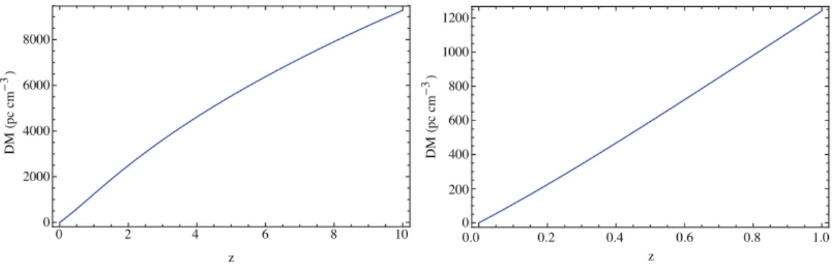
where the dispersion measure, DM, measures the column density of particles along the line of sight. 0 2 4 6 8 10 0 2000 4000 6000 8000 z D M pc cm 3 0.0 0.2 0.4 0.6 0.8 1.0 0 200 400 600 800 1000 1200 z D M pc cm 3
Figure 1: The contribution of the baryons present in the IGM to the DM of an ex-tragalactic pulse over (left) the redshift range 0 to 10, and (right) the range 0 to 1 in redshift.
For SKA-Low frequencies and with sources located at large cosmological distances, this delay can extend to thousands of seconds. The dispersion delay through our Galaxy can extend up to∼103
pc cm−3
for lines of sight near the Galactic plane, but is typically only ∼30 pc cm−3
for lines of sight above∼30◦ from the plane. The main contribution
to the dispersion measure for cosmological bursts emanates in the IGM, whose mean contribution can be computed as a function of redshiftz(see Ioka 2003, ApJ, 598, L79):
DM = 3cH0Ωb 8πGmp Z z 0 (1 +z′)dz′ p Ωm(1 +z′)3+ ΩΛ , (2)
where Ωb ≈ 0.04, Ωm = 0.3, ΩΛ = 0.7, H0 is the Hubble constant, G the gravitational constant andmp the proton mass. A plot of the DM contribution of the IGM is shown in
Figure 1. A useful analytic approximation that is correct to within 3% over the redshift range 0 to 1.0 is
DM≈1096(z+ 0.067z2) pc cm−3. (3) The exact contribution to the DM from the IGM is 1163 pc cm−3
for a burst atz= 1.0. This relation flattens at z > 1, and a search that extends to a DM of 3000 pc cm−3 extends out to a redshift z ≈ 2.7 if we assume that the DM contribution from our Galaxy and the host galaxy is negligible.
We adopt an upper limit of DM= 3000 pc cm−3
as a nominal upper limit to the range of dispersion measures we wish to be sensitive to. The Parkes radiotelescope, with a sensitivity modest compared to that of the SKA, has already detected FRBs with dispersion measures near 1500 pc cm−3
(Simon Johnston, private communication), which corresponds to z= 1.3. It is therefore reasonable to expect that the SKA will be able to readily detect bursts at roughly twice this redshift.
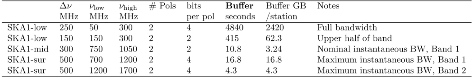
Table 1 lists the dispersion delay for each telescope and a selection of frequency ranges, for a cosmological burst with DM=3000 pc cm−3
. These represent nominal use-ful buffer sizes for detecting cosmological bursts out to redshifts ∼ 2.7, necessary to prosecute cosmological studies with Fast Radio Bursts.
∆ν νlow νhigh # Pols bits Buffer Buffer GB Notes
MHz MHz MHz per pol seconds /station
SKA1-low 250 50 300 2 4 4840 2420 Full bandwidth
SKA1-low 150 150 300 2 2 415 62.3 Upper half of band
SKA1-mid 300 750 1050 2 2 10.8 3.24 Nominal instantaneous BW, Band 1
SKA1-sur 500 700 1200 2 4 16.8 16.8 Maximum instantaneous BW, Band 1
SKA1-sur 500 1200 1700 2 4 4.3 4.3 Maximum instantaneous BW, Band 2
Table 1: Buffer requirements for each telescope to detect a burst with a dispersion measure of DM= 3000 pc cm−3
.
Backend data aggregation and network requirements
An additional requirement is the presence of a machine capable of aggregating the data acquired in the TBB and either processing it or archiving it for further analysis. Such a system should be capable of receiving and processing roughly one event per hour, in order to keep up with anticipated event rates2
. Whilst the computing demands are relatively modest, the storage requirements are large if the full capability of SKA-low is
2
The event detection rate is, of course, dependent on the telescope sensitivity and the characteristics of the events. The frequency at which the system can respond to triggers ultimately sets the detection threshold for transient event detections, and thus its sensitivity. A system which searches 500 dispersion measure trials in a data stream with 100µs time resolution would detect a 6.5σ “event” due to noise
once per hour, and would thus be able to search the data stream for real events that are brighter than 6.5σ. We also note that an event rate of∼10
4
events/per/sky for FRBs detected at Parkes implies that SKA-survey, in a coherent survey mode, would detect one FRB roughly every hour.
to be utilized. As shown in Table 1, an event at DM 3000 is seen more than an hour later at 50 MHz compared to 300 MHz, and storing the raw data from a single station requires over 2TB of storage. If the data from 1024 stations is stored, 2500 TB is required per event! In contrast, the requirements for SKA1-mid and SKA-survey are relatively modest - a single event requiring a maximum of 0.8 TB and 1.6 TB respectively.
In order to reduce the data volume of a single SKA-low event to a more manage-able size, less bandwidth or fewer antennas could be utilized. We note that this band-width/data rate trade-off was envisaged for LOFAR, but its implementation has been problematic after-the-fact, and this experience should inform the architecture from the outset. As shown in Table 1, taking only the top half of the band reduces the requirement to 62 GB per station per event. If the bandwidth were reduced further to 50 MHz, the required data volume shrinks further to 25 GB/station. If we assume these data need to be offloaded from the buffer within 30 minutes (in keeping with the goal of being able to react to∼1 event per hour) the total data rate to the transient processing machine would be 1024×62×8/1800 = 285 Gbps. Assuming the transient processing machine consists of a number of compute nodes with 40 Gbps Inifinband interconnect, this would demand 8 compute nodes for the most demanding case of SKA1-Low with 150 MHz of bandwidth. 3 nodes would suffice for SKA1-Low with 50 MHz of bandwidth, while a single node would suffice for SKA1-Mid (∼300 stations times 300 MHz) and SKA1-Survey (∼100 stations times 500 MHz bandwidth).
Once the data have been received, they must be correlated. This might be performed either by passing the data through the telescope correlator in a special mode or, more likely, by the data aggregation machine (or even off-site hardware). Scaling from the COBALT GPU correlator recently commissioned for LOFAR, a single GPU-enabled node can correlate 10 MHz of bandwidth for 80 stations in real time. Scaling this to 1024 stations with 150 MHz (the scaling is roughly quadratic with number of stations and linear with bandwidth) implies that the correlation process would take roughly 2400 times longer than realtime, or around 40 minutes to correlate one second of data. Since the transient signal occupies only a fraction of a second at any given frequency (and this is all that actually needs to be correlated - the cross-multiplication being the most costly part of the algorithm, and the only part which scales with number of stations squared) such a slowdown is acceptable given the desire to respond to∼1 event per hour, and the compute nodes which are required for aggregation will suffice to also do the processing. For SKA1-Mid with 3 times fewer stations but only twice the bandwidth, 2 nodes may be needed in place of the single node required by the networking. For SKA1-survey, with 10 times fewer stations and 5 times the bandwidth, a single node will suffice. We stress that this is based on performance fromcurrentsystems, and the systems available in ∼2020 should actually be considerably more powerful. A single dual-GPU node of the type used in COBALT costs ∼e15,000 in 2014, including networking cards. The networking switches necessary to pass data from the buffers to the aggregation/compute nodes would form an additional cost, but less than the nodes themselves. Accordingly, the total cost for the aggregation and processing system for SKA1-low, SKA1-mid and SKA-survey would be less than∼e300,000 euro in 2014 (dominated by SKA1-low), and
can be expected to fall by the time the systems would actually need to be purchased. Summary of requirements
∆ν duration Buffer Buffer with latency notes
MHz seconds GB GB
SKA1-low 150 415+10 62.3 63.8 upper half of band
SKA1-mid 300 10.8+10 3.24 6.24 Nominal instantaneous BW, Band 1
SKA1-sur 500 16.8+10 16.8 26.8 Maximum instantaneous BW, Band 1
SKA1-sur 500 4.3+10 4.3 14.3 Maximum instantaneous BW, Band 2
Table 2: Total buffer length requirements for each telescope to detect a burst with a dispersion measure of DM= 3000 pc cm−3
including a detection latency of 10 s, as specified in the Level 0 science requirements.
• The primary technical requirement is driven by the ability to buffer impulsive events with dispersion measures extending up to 3000 pc cm−3
.
– This places a severe requirement on the buffer length for SKA1-low, and it is suggested that in this case the buffer be capable of storing only the upper 150 MHz of the available band, which in turn requires a buffer length of duration∼7 minutes.
• Latency between the detection system and the buffer increases the size of the buffer over this minimum requirement. The level 0 science requirements specify that a latency of no longer than 10 s should be present in the system.
• In Table 2 we specify the required buffer sizesunder the assumption that the system
should buffer all data, taking account of the additional storage needed for latency.
However, we anticipate that the latency depends on the specifics of the backend architecture, and may be smaller than 10 s.
• The buffer should be able to respond to triggers from both a single-pulse detection machine (i.e. the pulsar detection machine)andfrom external triggers (e.g. events detected at other wavelengths, a gravitational wave event, or the SKA itself).
• In the event that no SKA-low pulsar search engine is available to feed triggers to the buffer, then the buffer data aggregation machine, described in the previous subsection, should subsume this role.
• A possible area of de-scope involves the buffering of fewer stations/antennas. The sensitivity of a transients search which detects events in the total-power streams of the station beamformers is smaller than the coherent sensitivity of the array by a factor Nstations1/2 . Thus, only the outputs ofN
1/2
stations need be buffered in order to achieve the same S/N as the triggering detection. We should emphasise that, as
buffer fulfills the crucial additional role of verifying each event, the buffer should ideally produce a (coherent) detection of each event with a S/N at least a factor of two higher than the triggering detection. We note that this tradeoff does not, of course, apply to events which are triggered externally.
• The station beamformers for SKA-low should be capable of outputting voltage data streams with a time resolution of less than 100µs. This may have implications for the filters used in the coarse channelisation stage in the station beamformers. (This may be a concern during EoR observations; in this instance a possible tradeoff is to abandon transients observations in the EoR observing mode, provided that the telescope does not operate in this mode more than∼30% of the time.)
• A secondary request, not discussed in detail in the present document, is to buffer the voltage outputs of the tied-array beamformer.
Additional remarks
Prior art: It is worth remarking that there are at least two recent notable implemen-tations of transients buffers:
• That used in the V-FASTR signal pipeline, in which the VLBA’s DiFX correlator outputs 1 ms antenna total powers which are dedispersed and searched for transient signals (Thompson et al. 2011, ApJ, 735, 98). If such a signal is found, the detection box triggers a dump of 1 s of baseband data from all the antennas being correlated corresponding to the time of the event.
• The transient buffer boards installed in LOFAR. TBBs have been an integral com-ponent of the LOFAR design dating back to its inception. However, to this day the transient buffers installed in LOFAR are not routinely used in transients detection pipelines. Thus, the LOFAR case seems to present an example of a way in which
not to implement a transients buffer. The main cause of this failure seems to be related to the failed development of software and firmware to support the readout and processing of the TBBs. This, in turn, appears to be attributed to the failure of a “Level 0” system design requirement to propagate into appropriate directives in more specific technical documentation (i.e. the Level 1 and 2 system design specifications).
RFI mitigation: We note that the transient buffers and searches occur exactly where one wants to perform RFI detection and removal/flagging. Adding the option of transient support there would also contribute to sophisticated RFI removal or flagging.
System readiness: We realise that it may be possible to implement a fully-capable TBB for all three SKA telescopes in the re-baselined SKA1. However, in this instance, we request that the system be design with appropriate data spigots to permit the future attachment of transient buffers.
Technical Feasibility
We discuss possible implementations of transient buffers on each of low, SKA1-mid and SKA1-survey separately below. The cost of implementation is necessarily architecture-specific; here we suggest ways in which a Transients Buffer Board (TBB) may be implemented zero or minimal additional cost.
The primary aim is to buffer the station voltages for SKA1-low, the antenna voltages for SKA1-mid and the PAF voltages for SKA1-Survey. This is necessary for localisation of transients within the primary FoV of each station, antenna or PAF element.
A secondary request is the ability to buffer tied-array voltages so as to enable the recovery of a signal, including its polarization.
SKA1-low implementation
SKA requirement 2636 states that “SKA1-low shall be capable of outputting beam prod-ucts as voltage time series.” Granted this, the main remaining issue is then the provision of some continuously-cycling buffer capable of storing the requisite duration of data.
Given the buffer sizes required (Table 1), and the data bit rates from each station, Table 2 presents the bit rate, disk size and durability estimates for an SKA1-Low imple-mentation with 1 TB solid-state drives (SSDs). This is a possible architecture solution proposed for SKA1-Low. A single SSD would serve a single station, and access the beamformed voltages (not channelized). We emphasise that SSDs are only an example storage medium; other options may be more appropriate and durable, such as DRAM attached to the beamformer nodes3 Estimates are provided for use of the (1) full array (1024 stations, 8-bit sampling, 250 MHz bandwidth), and (2) reduced array using all core stations and 8 outriggers for localization precision (520 stations, 2-bit sampling, 150 MHz bandwidth).
Costings Cost/1TB disk No. disks Cost per year (e)
Full e100 1024 e48439
Reduced e100 520 e4380
Table 3: Cost estimates for SKA-Low SSD implementations.
Although the Baseline Design specifies 8-bit sampling for data to the correlator for SKA-Low, 2-bit sampling would be adequate for the TBBs. In addition, the moderate gain in sensitivity of extending the SKA-Low lower frequency to as low as 50 MHz is likely to be impacted by low-frequency scattering. An implementation which records only the upper portion of the band would substantially reduce the length of buffer required.
3
A suggestion, due to John Bunton, is that the buffer may instead by implemented in the memory used for the corner-turning operation prior to correlation. DRAMs of up 128 GB are currently available on the market, and would be suitably large as buffers, even for SKA1-low (buffering the upper half of the band). The high I/O throughput of the corner-turning operation means that this hardware necessarily has the large bandwidth suitable for dumping the buffer contents to a secondary storage device.
This costing is based on the estimate ofe100 per 1TB SSD. We note that the pricing of SSD devices changes rapidly. Between April 2013 and April 2014 the price fell from e430/TB toe330/TB, suggesting that a unit cost ofe100 is realistically achievable by 2017.
SKA1-survey implementation
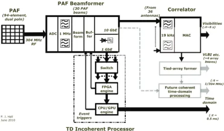
It is likely that a transients buffer can be implemented for SKA-survey inside the PAF beamformers at zero additional hardware cost. Beamforming of the voltage streams from each of the receivers on each PAF will require dedicated high-throughput hardware before it is sent to the correlator, and this hardware will contain some form of volatile memory. A concrete example is the ASKAP beamformer, which is currently implemented on dedicated FPGAs. Each FPGA includes several GB of DRAM which holds a ring buffer of the beamformed voltages for each sub band and each telescope. Thus, in effect, the ASKAP architecture automatically provides a continuous buffering capability. A schematic of a fast transients voltage buffer for ASKAP is shown in Figure 2.
The issue of buffering is therefore simply one of access to the beamformer memory. The required buffers for SKA-Sur are small (<20 seconds) and existing backend architec-ture can be used to hold data in memory for PAF beamforming. Small, durable external SSDs can be implemented to capture stored data when a trigger occurs, with minimal additional cost.
Costing Cost/1TB disk # disks Cost per year (e)
SKA1-mid 100 254 24030
Table 4: Cost estimates for an SKA-Mid SSD implementation.
SKA1-mid implementation
For SKA-Mid, as shown in Table 1, the buffer lengths required are minimal compared with those required for SKA1-low. The proposed implementation is to either (1) use existing architecture, which will be holding data in memory for beamforming, or (2) use external SSDs. For a nominal 300 MHz bandwidth and 2-bit sampling, Table 3 lists the capacities required and lifetimes.
DM Pols Nbits per pol Buffer length I/O Rate† SSD size req’d Lifetime of 1TB disk
pc cm−3
seconds Gbits/second GB Days (P/E= 105 )‡
3000 2 2 10.8 2.40 3.25 386
Table 5: SKA-Mid buffer requirements. Notes: † Npols×Nbits×2×Bandwidth (Nyquist). ‡ P/E ratio = number of write and erase cycles before disk failure.
MAC (From 36 antennas) Correlator Tied-array former Visibilities ( t~5 s) VLBI etc. (~4 array beams) Future coherent time-domain processing Time domain ( t ~ 1/304 MHz) ( t ~ 0.5 ms) 19 kHz PAF (94-element, dual poln) ADC 1 MHz Beam form Switch FPGA engine CPU/GPU engine PAF Beamformer (30 PAF beams) 1 GbE Event triggers 304 MHz RF 10 GbE TD Incoherent Processor Buf-fer P. J. Hall June 2010
Figure 2: A schematic of the fast transients processing solution proposed for ASKAP. 1-ms timescale beam powers are aggregated inside the PAF beamformers and despatched via the 1GbE port to a commodity switch. This combines the signals from all beamform-ers (all telescopes and all frequencies) and relays them to an FPGA-based dedispbeamform-ersion and detection system. Upon detection of an event, a trigger is relayed back to the beam-former, which initiates a data dump of a small section of data from the beamformer DRAM via a spare 10GbE port either to offline storage or to the coherent time-domain processor, which performs the compute-intensive task of searching for the position of the event at the (known) DM and start time of the transient.
Storage medium durability
For SKA-Low and -Mid, SSDs are suggested here as an example of a cost-effective and durable storage medium. SSDs have a maximum number of write-erase cycles before disk failure (the P/E ratio). For a nominal P/E and current costings for a 1 TB disk, Table 4 lists the approximate costings per year. Costs are provided for use of the full array with 2-bit sampling and 300 MHz bandwidth.
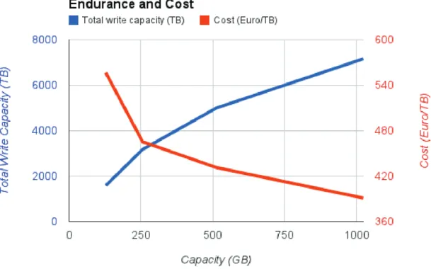
The smaller buffer sizes necessary for SKA1-mid and -survey permit the use of smaller capacity memory devices. In principle, a device with only 5GB memory would suffice to buffer the signals from these instruments. However, for some storage media dura-bility plays an important role in the cost estimate. A larger-capacity SSD undergoes fewer write/erase cycles per unit time for a given buffer size, and therefore has a longer operational lifetime. The lifetime must be offset against the cost of the larger-capacity disk. Thus there is a tradeoff between the unit cost of each SSD as a function of ca-pacity and its expected lifetime. For instance, one might opt to implement the buffer using 100GB SSDs, but if these only last one tenth the time of 1TB SSDs they will only be cost effective if they cost less than one tenth of a 1 TB SSD. With the advent of high-capacity, high-performance, durable Single-Level Cell (SLC) drives, there are commercially-available options to meet the demands of SKA. Figure 3 shows the cost
effectiveness of various implementations as a function of SSD unit size based on current pricing and P/E lifetimes. It demonstrates that high-capacity disks are an effective so-lution. Beyond the variable costs of disk replacement, larger disks also require less cost overhead from the manpower required to physically replace failed drives.
Figure 3: A graph of the expected total write capacity and cost per terabyte, of a transients buffer implemented using SSDs against the capacity of the individual SSDs comprising the system.