Malware Detection Using Dynamic Analysis

San Jose State University

SJSU ScholarWorks

Master's Projects Master's Theses and Graduate Research

Spring 5-25-2015

Malware Detection Using Dynamic Analysis

Swapna Vemparala

San Jose State University

Follow this and additional works at:https://scholarworks.sjsu.edu/etd_projects

Part of theArtificial Intelligence and Robotics Commons, and theInformation Security Commons

This Master's Project is brought to you for free and open access by the Master's Theses and Graduate Research at SJSU ScholarWorks. It has been accepted for inclusion in Master's Projects by an authorized administrator of SJSU ScholarWorks. For more information, please contact

Recommended Citation

Vemparala, Swapna, "Malware Detection Using Dynamic Analysis" (2015).Master's Projects. 403. DOI: https://doi.org/10.31979/etd.48fu-qckf

Malware Detection Using Dynamic Analysis

A Project Presented to

The Faculty of the Department of Computer Science San Jose State University

In Partial Fulfillment

of the Requirements for the Degree Master of Science

by

Swapna Vemparala May 2015

c ○2015 Swapna Vemparala ALL RIGHTS RESERVED

The Designated Project Committee Approves the Project Titled

Malware Detection Using Dynamic Analysis

by

Swapna Vemparala

APPROVED FOR THE DEPARTMENTS OF COMPUTER SCIENCE

SAN JOSE STATE UNIVERSITY

May 2015

Dr. Mark Stamp Department of Computer Science Dr Thomas Austin Department of Computer Science Fabio Di Troia Università del Sannio

ABSTRACT

Malware Detection Using Dynamic Analysis

by Swapna Vemparala

In this research, we explore the field of dynamic analysis which has shown promis-ing results in the field of malware detection. Here, we extract dynamic software birth-marks during malware execution and apply machine learning based detection tech-niques to the resulting feature set. Specifically, we consider Hidden Markov Models and Profile Hidden Markov Models. To determine the effectiveness of this dynamic analysis approach, we compare our detection results to the results obtained by using static analysis. We show that in some cases, significantly stronger results can be obtained using our dynamic approach.

ACKNOWLEDGMENTS

I am very thankful to my advisor Dr. Mark Stamp for his continuous guidance and support throughout this project. Also, I would like to thank my committee members Dr. Thomas Austin and Fabio Di Troia for their feedback and guidance. Last but not least, I would like to express my gratitude to my family for their support.

TABLE OF CONTENTS CHAPTER 1 Introduction . . . 1 2 Background . . . 4 2.1 Types of Malware . . . 4 2.1.1 Virus . . . 4 2.1.2 Trojan . . . 7 2.1.3 Worm . . . 7 2.1.4 Backdoor . . . 8

2.2 Static Anti-Virus Techniques . . . 8

2.2.1 Signature Based Detection . . . 8

2.2.2 Static Heuristics Analysis . . . 9

2.3 Dynamic Anti-Virus Techniques . . . 9

2.3.1 Behavior Blocker . . . 9

2.3.2 Emulators . . . 10

2.4 Hidden Markov Model Based Detection . . . 11

2.5 Profile Hidden Markov Model Based Detection . . . 15

2.6 Analysis Techniques . . . 25

2.6.1 Static Analysis . . . 25

2.6.2 Dynamic Analysis . . . 26

2.7 Previous Work . . . 26

2.7.2 Graph Based Technique . . . 27

2.7.3 API Calls Based Techniques . . . 27

2.7.4 Operand Stack Runtime Based Technique . . . 28

3 Implementation . . . 29

3.1 HMM . . . 29

3.1.1 Dynamic Analysis Technique . . . 29

3.1.2 Static Analysis Technique . . . 30

3.2 PHMM . . . 31

3.3 Chosen Dataset . . . 32

3.4 Tools Used In the Project . . . 34

3.4.1 Tools Used for Dynamic Analysis . . . 34

3.4.2 Tools Used for Static Analysis . . . 35

4 Experiments and Results . . . 36

4.1 Setup . . . 36

4.2 Results . . . 36

4.2.1 Receiving Operating Characteristics . . . 37

4.2.2 Hidden Markov Model . . . 37

4.2.3 Profile Hidden Markov Model . . . 40

5 Conclusion and Future work. . . 44

APPENDIX A Dynamic Analysis Results . . . 49

LIST OF TABLES

1 Masquerade detection example with PHMM [23] . . . 18

2 PHMM Pairwise Alignment [23] . . . 19

3 MSA [23] . . . 20

4 Emission Probabilities for the MSA in Table 3 . . . 22

5 Transition Probabilities for the MSA in Table 3 . . . 23

6 Benign files . . . 33

7 Benign files . . . 34

8 AUC curve results for static and Dynamic Analysis . . . 40

LIST OF FIGURES

1 Dynamic Signatures [4] . . . 10

2 Hidden Markov Model [22]. . . 11

3 Profile Hidden Markov Model [23]. . . 16

4 ROC Curve . . . 37

5 Security Sheild: Scatterplot . . . 38

6 Security Shield: Area Under the Curve . . . 38

7 Security Shield: Scatterplot . . . 38

8 Security Shield: Area Under the Curve. . . 39

9 Zeroaccess PHMM ROC -all groups . . . 41

10 PHMM results -all groups . . . 42

11 HMM and PHMM Comparison -all groups . . . 42

A.12 ZBOT: Area Under the Curve. . . 49

A.13 Security Shield: Area Under the Curve. . . 49

A.14 Harebot: Area Under the Curve. . . 49

A.15 Smarthdd: Area Under the Curve. . . 50

A.16 Winwebsec: Area Under the Curve. . . 50

A.17 Zeroaccess: Area Under the Curve. . . 50

A.18 Cridex: Area Under the Curve. . . 50

B.19 ZBOT: Area Under the Curve. . . 51

B.20 Security Shield: Area Under the Curve. . . 51

B.22 Smarthdd: Area Under the Curve. . . 52

B.23 Winwebsec: Area Under the Curve. . . 52

B.24 Zeroaccess: Area Under the Curve. . . 52

B.25 Cridex: Area Under the Curve. . . 53

C.26 Cridex PHMM ROC -all groups . . . 54

C.27 Harebot PHMM ROC -all groups . . . 54

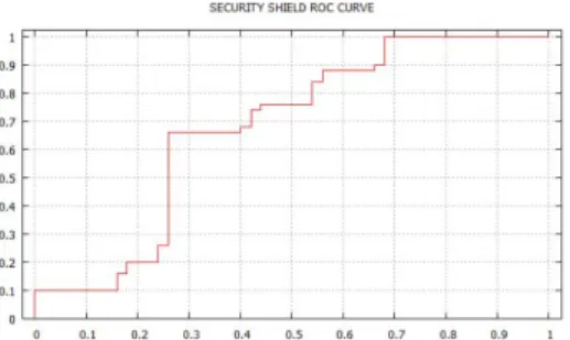
C.28 Security Shield ROC -all groups . . . 55

C.29 SmartHhdd PHMM ROC -all groups . . . 55

C.30 Zeroaccess PHMM ROC -all groups . . . 56

C.31 Winwebsec PHMM ROC -all groups . . . 56

CHAPTER 1 Introduction

Malicious software or malware are harmful software that are designed to harm computers or computer networks. Malware attacks have become a major threat to the world. This is a major concern in the consumer space as hackers try to get personal information of users, steal their identities to make money and use them for other nefarious activities.

To cite a few examples, Twitter a popular social networking company that re-cently went public was in the news for the wrong reasons. This newly formed company was at the receiving end of a major cyber attack. According to news reports 250,000 users’ email addresses, user names and passwords were compromised. Twitter was able to detect the live attack by identifying the abnormal patterns in which the data was accessed [11].Target fell victim to a major security breach during the 2013 holiday season, which is believed to be one of the biggest retail security breaches in United States. This breach compromised the personal information including credit and debit card details of a whopping million customers. The information was stolen by hack-ing the credit card swipe systems at Target stores [10]. This one attack drove down quarterly revenues of Target by tens of millions of dollars [33].

In today’s world of malware and cyber threats, it has become critical to develop techniques that quickly detect and eradicate malware. This is important for businesses and consumers alike. In this paper, we look at different malware detection techniques and compare their results. Based on the results the best detection techniques will be identified.

In this research we use the concept of software birthmarks for malware detection. Software birthmarks are inherent characteristics that is used to identify a particular software [18, 31]. The basic idea here is to obtain a "software birthmark", which is a unique identifier of a software. Having obtained the software birthmark for each software, one can use this to test the similarity between the two software. If the two birthmarks are the same, the similarity in the birthmarks implies that one software is a copy of another. Based on this, there has been a lot of research in the field of software birthmarks [12, 14, 18, 21, 31, 32, 35, 36].

Software birthmarks can be either static or dynamic [12]. Static birthmarks are characteristics that can be extracted from a program without executing it [36]. For example, a static birthmark can be based on an extracted opcode sequence. In contrast, dynamic birthmarks are obtained from a program when it is executed [14, 31, 36]. An example of a dynamic birthmark is the sequence of API calls that occur when a program is executed [32].

This project extends previous work involving static birthmarks for malware de-tection [32] to dynamic birthmarks. We employ a variety of machine learning tech-niques, including Hidden Markov Models (HMMs) and Profile Hidden Markov Mod-els (PHMMs). To determine the effectiveness of our dynamic analysis techniques, we compare static and dynamic analysis results on substantial malware datasets using Receiving Operating Characteristics(ROC) analysis [7]. We show that significantly stronger malware detection results can be obtained using dynamic analysis of software birthmarks, as compared to static analysis.

The remainder of this paper is organized as follows. In Chapter 2, we provide background information on types of malware and detection techniques. Here we discuss in detail about the two main machine learning based techniques used in this

project, Hidden Markov Model based detection and Profile Hidden Markov Model based detection. In Chapter 3, we discuss the implementation details for this project. Here we discuss in detail about the tools used for extracting the data, the dataset used and we also explain in detail the implementation of the machine learning techniques used in this project. The experiments and discussion of the results are outlined in Chapter 4. This paper concludes with Chapter 5 that discusses the conclusion and future work.

CHAPTER 2 Background

Malware is a generic term that encompasses viruses, worms, backdoor and tro-jans. Next we will be discussing about the different types of malware in detail.

2.1 Types of Malware 2.1.1 Virus

Virus is a malware that has a self replicating nature. It is constructed to modify or stop the functioning of a computer. It multiplies by first infecting one program. When this program is executed the virus tries to insert another version of itself into another program. A virus can locate itself within multiple areas of a system such as boot sector,hard drives and programs [1, 4]. An example for a virus is a macro virus, when the word document is infected by this virus and is opened by a user, the macros inside the document gets executed, allowing the virus to gain control [4]. In the year 2010, a destructive virus called the Stuxnet virus was created. It was primarily developed to target industrial control systems which are used in power plants. This malware was designed to modify and control the programmable logic controllers present in the control systems in the way the attackers needed [30].

2.1.1.1 Encrypted Virus

These viruses are designed to evade signature based detection techniques used in Antivirus software as encryption hides the actual signature of the malware. In an encrypted virus, the body of the virus is encrypted to evade detection. In order for the virus to run it has to decrypt itself before running the actual virus program. This

is done by means of the decrypter loop present in the virus. The type of encryption can be done by means of a static or a variable key or a simple bitwise rotation or by incrementing or decrementing the bits in the virus body [4]. The basis for selecting the decrypter algorithm is to choose a simple algorithm that can evade pattern based detection. Also since the decrypter code is not encrypted choosing a complex algorithm does not provide any benefit. The first encrypted virus was the DOS virus Cascade [34].

2.1.1.2 Polymorphic Virus

A polymorphic virus is also similar to the encrypted virus. The difference is that the decrypter loop changes in each generation unlike in the case of an encrypted virus whose decrypter loop remains constant. Once the decrypter code gains control of the host computer it decryptes the body of the virus after which the virus program can run [27]. This virus can have up to a million decrypter loops with the help of a mutation engine and hence they are harder to detect compared to the encrypted viruses [4]. Hence this virus can evade detection by Antivirus software as it has no specific signature and no constant decryptor code that can help in the identification process. The polymorphic viruses are indeed hard to detect. Over the past few years, detection techniques have been developed that wait for the virus to decrypt itself before detecting it [15]. In 1991 the first polymorphic Tequila and Maltese Amoeba viruses were detected [27].

2.1.1.3 Metamorphic Virus

These viruses unlike the viruses stated in the above two subsections are not encrypted. The detection of metamorphic viruses is pretty challenging. They are

more advanced compared to the encrypted and polymorphic viruses. These viruses make use of a mutation engine in order to morph its body at each generation but the basic functionality of the virus remains unchanged [4]. Metamorphic viruses can make use of different methods to morph the internal structure. A few of the methods are discussed below.

1. Dead Code Insertion

This is a simple technique used in many of the metamorphic viruses. The idea here is to insert dead code in such a way that it does alter the functionality of the code. The Win32/Evol virus, which was created in 2000, is an example of a virus that has a metamorphic engine that would insert garbage code [15]. 2. Instruction Reordering

This involves reordering of the instructions as long as the reordered instructions do not have a dependency on the previous ones. Since no dependency is broken instruction reordering does not affect the functionality of the virus but provides a lot of morphed copies.

3. Instruction Substitution

This involves replacing a group of instructions by their equivalent ones. Hence the functionality of the malware remains unchanged but we derive a morphed version of the body [4].

4. Register Swapping

In this technique the virus body is morphed by swapping operand registers with different registers. Though the virus body is mutated this technique does not change the opcode sequence as swapping techniques only changes the register

names. An example for a metamorphic virus that used register swapping is the W95/Regswap virus that was created back in 1998 [15].

2.1.2 Trojan

A trojan is a malware that looks innocuous to the user but performs malicious activities in the background and unlike a virus it is a standalone programs. It is not self-replicating in nature and is user dependent for its propagation. As an example, an attacker can create a login program that prompts the user to enter the username and password. If the user mistakenly enters his or her credentials, the program steals the users credentials by displaying an invalid message and in the second attempt the actual login program is run [4]. Trojans are very harmful as the user is completely unaware of the malicious activities that take place in the background. Trojans constitute a major portion of the today’s malware activity [15].

2.1.3 Worm

A worm is a malware that is similar to a virus. A worm differs from a virus in the way it spreads to different systems through the network. Worms are not parasitic in behavior like the viruses. They are independent programs that can cause harm on their own. These worms may or may not have a payload but both types can be pretty harmful. Worms without payloads does not affect the system that it infects. Whereas the worms with payload will do harm to the infected system as well. In some cases the payload acts as a backdoor instead of making changes to the system. The backdoor in the user’s system can be used to steal users’ personal information or credentials. The Morris worm created in 1988 was one of the earliest worms that was created. In the year 2000, the SQL Slammer worm caused great disruption to

computers that were connected to the internet and had Microsoft SQL Server running on their machines [15].

2.1.4 Backdoor

A backdoor is a malware that is used to bypass normal security authentication processes. After gaining access, it takes control of the system and can remotely control and monitor it while stealing personal information [4]. An example for a backdoor malware is Back Orifice [8]. This malware on gaining control of the infected system can download, upload or delete files, lock or shutdown the computer, or even take control of the keyboard and mouse [24].

2.2 Static Anti-Virus Techniques 2.2.1 Signature Based Detection

Signature based detection technique is used by many anti-virus products. This involves scanning through the files in your system in search of a specific set of pat-terns. The anti-virus products have a database of patterns or signatures and if a match is found then that file is classified as a malware. The key to a good signa-ture based detection is that the database of signasigna-tures has to be updated frequently otherwise newly added malware can go undetected. Though this technique can help in identifying the detected malware, some of the more sophisticated malware such as metamorphic, encrypted and polymorphic viruses can easily evade this type of detection [4].

2.2.2 Static Heuristics Analysis

Unlike signature based detection static heuristics does not identify malware by scanning signatures. Instead it analyses the behavior, structure and other attributes for virus-like qualities [4]. This technique can be used to identify zero-day malware as well as existing malware. This method identifies the probability of a file being infected by performing an in depth analysis of the instructions, logic of the program, data used and overall structure of the binary file it scans. There are heuristic scanners that are available in the industry that have a high detection rate of 70% to 80%. On the pros side, static heuristics analysis has the ability to detect malware even before they can infect the computer. On the con side, an inefficient heuristics scanner can results in multiple false positives where a benign file is wrongly identified as a malware [28].

2.3 Dynamic Anti-Virus Techniques 2.3.1 Behavior Blocker

Behavior blocker executes the program and closely monitors it for suspicious activities. If a suspicious activity is encountered, the behavior blocker will stop the program [4]. Unlike static based detection techniques the dynamic based detection techniques need to only consider the instructions that have been executed. The behavior blocker takes advantage of this fact and hence focuses on the calls that are obtained when the code gets executed, since dead code becomes irrelevant as it never gets executed. Behavior blockers make use of dynamic signatures. The dynamic signatures are created by collecting the calls that are obtained when executing a malware. The calls are then grouped over a window of size k. Figure 1 gives an example of a dynamic signature of length 𝐾 = 3.

Figure 1: Dynamic Signatures [4]

2.3.2 Emulators

Unlike in the case of behavior blockers the emulators do not run the malware directly in the system, instead they run it in an emulated environment which is a safe virtual environment. The emulators make use of dynamic heuristics which collect the information about the malware that is being executed in an emulated environment. The information collected by dynamic heuristics can include the requests made to the operating system by the malware which form the dynamic signatures. Given the fact that dynamic heuristics closely monitor the operating system, they have a significant advantage over static heuristics in detecting virus that target operating systems. On the negative, side the CPU emulation process is much slower compared to the signature scanning process and hence the dynamic heuristics is slower than static heuristics. Also some viruses employ logic tricks and hide its infection logic from the emulator by performing the infection only under specific conditions, which prevents the dynamic scanner for detecting the malware [28].

2.4 Hidden Markov Model Based Detection

Hidden Markov models (HMMs) are generally used for statistical pattern anal-ysis. They have been proven to do well in the fields of speech recognition, biological sequence analysis [1] and software piracy detection [21]. In this project we extend the Hidden Markov Model machine learning technique to perform malware detection using dynamic analysis. A Markov process is a memoryless process that depends only on the present state. A HMM is used to model a system that is assumed to be a Markov process with hidden states. In HMM since the state is hidden the user can only observe the output. The output is dependent on the hidden state. Each state has an associated probability distribution for a set of observations. The transition probabilities between the states are fixed. Using the observation sequences that is ob-tained from the malware(in the case of this project) the HMM can be trained. After training we can test the observation sequence against a trained HMM to determine the likelihood of the sequence being a part of the model. A high probability indicates a good match [1].

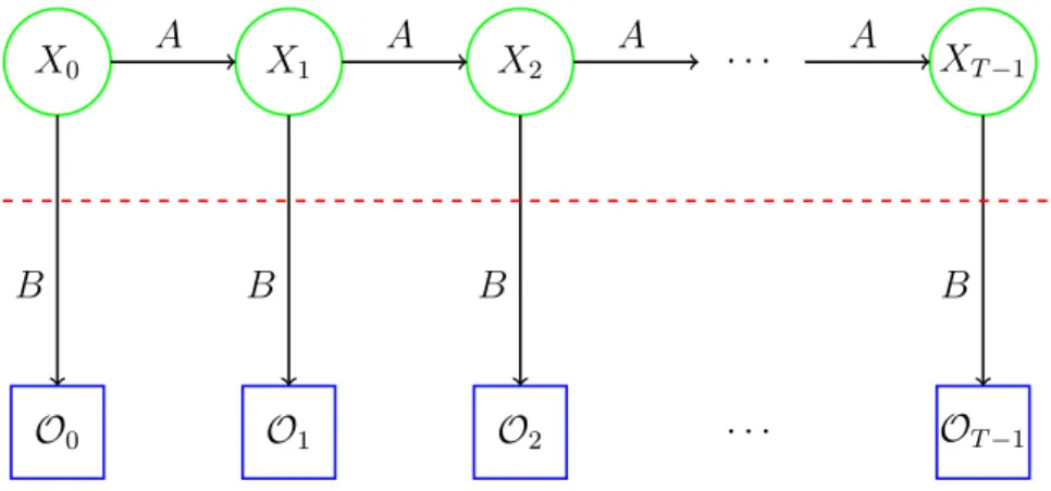
Figure 2 represents a typical Hidden Markov Model. The notations used for in the Hidden Model are shown below Figure 2:

𝒪0 𝒪1 𝒪2 · · · 𝒪𝑇−1

𝑋0 𝑋1 𝑋2 · · · 𝑋𝑇−1

𝐴 𝐴 𝐴 𝐴

𝐵 𝐵 𝐵 𝐵

𝑇 = length of the observation sequence

𝑁 = number of states in the model

𝑀 = number of observation symbols

𝑄 = {𝑞0, 𝑞1, . . . , 𝑞𝑁−1}=distinct states of the Markov process 𝑉 = {0,1, . . . , 𝑀 −1}=set of possible observations

𝐴 = state transition probabilities

𝐵 = observation probability matrix

𝜋 = initial state distribution

𝒪 = (𝒪0,𝒪1, . . . ,𝒪𝑇−1) =observation sequence.

A HMM is represented as 𝜆 = (A,B, 𝜋). In figure 2, 𝑋𝑖 represent the hidden states. As mentioned above the Markov process is hidden and is determined by the𝐴matrix and present state. The observations 𝒪𝑖 are visible and are related to the hidden states, hence we can indirectly obtain information about the hidden states. These observations are related to B matrix [22].

The HMM can be used to solve three basic problems that are listed below.

1. Problem 1: When given a model 𝜆= (A,B, 𝜋) and a observation sequence, we can determine the likelihood of the sequence in that model [22].

2. Problem 2: Given a model𝜆 = (A,B, 𝜋)and an observation sequence𝒪, we can determine an optimal state sequence for the Markov model. We can determine the most likely hidden sequence [22].

3. Problem 3: When given a observation sequence we can generate the model 𝜆

such that it maximizes the probability of the observation sequences [22].

We use problem 3 for training the HMM in our project. We use the sequences that we obtain from the malware dataset and append them after which we send them to the HMM for training. We then use problem 1 for testing where we use the sequences from

benign datasets to check if the model can classify malware from benign files. Next we will look at the algorithms used to solve the problems listed above. The forward algorithm, backward algorithm and Baum-Welch re-estimation algorithm are used during the training phase and to perform the scoring we used the forward algorithm. The forward algorithm computes 𝑃(O|𝜆). It is also known as the alpha pass algorithm. We can state the algorithm as [22]:

1. For 𝑡 = 0,1, . . . , 𝑇 −1and 𝑖= 0,1, . . . , 𝑁 −1

2. 𝛼𝑡(𝑖) = 𝑃(𝒪0,𝒪1, . . . ,𝒪𝑡, 𝑥𝑡=𝑞𝑖|𝜆)

The partial observation sequence until time 𝑡 has the probability as 𝛼𝑡(𝑖). This value is computed recursively using the following forward algorithm approach.

1. For 𝑖= 0,1, . . . , 𝑁 −1, let

𝛼0(𝑖) = 𝜋𝑖𝑏𝑖(𝑂0)

2. For 𝑡 = 0,1, . . . , 𝑇 −1and 𝑖= 0,1, . . . , 𝑁 −1, compute

𝛼𝑡(𝑖) = [︃_𝑁−1 ∑︁ 𝑗=0 𝛼𝑡−1(𝑗)𝑎𝑗𝑖 ]︃ 𝑏𝑖(𝒪𝑡)

3. The probability of the observation sequence in the model is given by

𝑃(𝒪|𝜆) =

𝑁−1

∑︁

𝑖=0

𝛼𝑇−1(𝑖)

Problem 2 can be solved using the backward algorithm also know as beta pass [22]. This is opposite to the forward algorithm as it works in reverse. The algorithm is given below

2. 𝛽𝑡(𝑖) =𝑃(O𝑡+1,O𝑡+2, . . . , 𝑂𝑇−1, 𝑥𝑡=𝑞𝑖, 𝜆)

This value is computed recursively using the following approach.

1. Let 𝛽𝑇−1(𝑖) = 1, for 𝑖= 0,1, . . . , 𝑁 −1, 2. Compute 𝛽𝑡(𝑖) = 𝑁−1 ∑︁ 𝑗=0 𝑎𝑖𝑗𝑏𝑗(𝒪𝑡+1)𝛽𝑡+1(𝑗)

For𝑡 =𝑇 −2, 𝑇 −3, . . . ,0 and 𝑖= 0,1, . . . , 𝑁 −1 and

𝛾𝑡(𝑖) =𝑃(𝑥𝑡=𝑞𝑖|𝒪, 𝜆) For𝑡 = 0,1, . . . , 𝑇 −1and 𝑖= 0,1, . . . , 𝑁 −1,

Having computed 𝛽𝑡(𝑖)and 𝛼𝑡(𝑖)we can determine the probability upto time t by:

𝛾𝑡(𝑖) =𝛼𝑡(𝑖)𝛽𝑡(𝑖)/𝑃(𝒪|𝜆)

The final algorithm that is discussed here is the Baum-Welch algorithm. In this algorithm the parameters 𝐴, 𝐵 and 𝜋 are iteratively re-estimated [22]. Problem 3 is solved using this approach.

1. Step1. We first Initialize 𝜆 = (A,B, 𝜋) to random non uniform values. The values can be chosen such that 𝜋𝑖 ≈1/𝑁,𝐴𝑖𝑗 ≈1/𝑁 and 𝐵𝑗𝑘 ≈1/𝑀.

2. Step2. Then, we compute 𝛼𝑡(𝑖), 𝛽𝑡(𝑖), 𝛾𝑡(𝑖) and 𝛾𝑡(𝑖, 𝑗). where

For𝑡 = 0,1, . . . , 𝑇 −1and 𝑖, 𝑗 ∈ {0,1, . . . , 𝑁 −1} and

𝛾𝑡(𝑖, 𝑗) =

𝛼𝑡(𝑖)𝑎𝑖𝑗𝑏𝑗(𝒪𝑡+1)𝛽𝑡+1(𝑗)

𝑃(𝒪|𝜆) .

where di-gammas is the probability of transitioning from state 𝑞𝑖 at time 𝑡 to state 𝑞𝑗 at time 𝑡+ 1. 𝛾𝑡(𝑖) = 𝑁−1 ∑︁ 𝑗=0 𝛾𝑡(𝑖, 𝑗)

the above equation shows the relation between di-gammas and𝛾𝑡(𝑖) 3. Step3. Re-estimate the HMM model 𝐴, 𝐵 and 𝜋.

4. Step4. If 𝑃(𝒪|𝜆)increases, then repeat step 2.

This process is stopped when 𝑃(𝒪|𝜆) does not increase after a certain number of iterations or threshold [22].

In Chapter 3 we will discuss in detail the implementation of the HMM discussed here in our project.

2.5 Profile Hidden Markov Model Based Detection

Profile Hidden Markov Model(PHMM) is a probabilistic technique that is widely used in the field of Bioinformatics. As an application, a Profile Hidden Markov model could be created by aligning several protein families and this model can be used to identify the similarity between given unknown protein sequences and the generated model [20]. An application for this can be obtained in software packages that are available like HMMER, SAM, PFTOOLS etc. The Profile Hidden Markov Model technique has unique advantages over the Hidden Markov Model(HMM) technique. It takes into account the positional information in the sequences used for training

training. Given the statistical nature of the HMM the position of the sequences are inconsequential. Also unlike PHMM the HMM does not take into account the insertions and deletions in a sequence which are important in certain applications [9]. The goal in this project is to test the effectiveness of the PHMM technique in the field of malware detection using dynamic analysis. The training sequence considered here are the API calls that are obtained by executing the malware. After the PHMM model has been created the model will be used to test if a given sequence belongs to the family or not. It will be tested for malware sequences that belong to the same family and benign sequences.Figure 3 represents a PHMM.

begin 𝑀1 𝑀2 𝑀3 𝑀4 end

𝐼0 𝐼1 𝐼2 𝐼3 𝐼4

𝐷1 𝐷2 𝐷3 𝐷4

Figure 3: Profile Hidden Markov Model [23].

The rectangles depict the match states. These states as are used to compute a probability distribution as they have sufficient information to do so. The diamonds in the figure depict the insert states. The circles depict the delete states. This is discussed in more detail below. The first step in creating the PHMM is aligning the sequence to build a multiple sequence alignment(MSA). This is equivalent to the training step in HMM. A pairwise alignment technique is used to align the sequences that are obtained from the training set. In this technique a pair of sequences are

considered and an attempt is made to align the symbols in the sequences. In the case where the sequences are not similar, gaps are introduced to bring about the alignment. A special symbol ‘-’ is introduced to represent the gaps. In this project the training datasets consists of the API calls that are obtained by executing the malware. In order to perform the pairwise alignment on the dataset some amount of preprocessing is required.

In the preprocessing step, we followed [3] where the API calls are first sorted by the frequency of occurrence in a particular malware family and the top 36 API calls are considered. These top 36 API calls constitute 99.8% to 100% of the total API calls in a given family. These API calls are then mapped to the letters in the English alphabet[A-Z] and numbers[0-9]. All the remaining API calls will are mapped to an asterisk symbol ‘*’ [3]. This preprocessing step simplifies the process of performing a pairwise alignment to the dataset in consideration.

The next step is creating a substitution matrix. This matrix consists of scores for all the possible alignment of symbols. The approach used for creating the substitution matrix is similar to the approach used in [3]. If two symbols are alike then a high positive score will be assigned. In the case where both symbols are ‘*’ a medium positive score is assigned .Finally for the case where both the symbols are different a low negative score is assigned.

For a better understanding of the PHMM technique we will proceed with the rest of discussion on PHMM by using the example of masquerade detection problem discussed in [23]. The goal in masquerade detection is to be able to identify an attacker that would act as a genuine user to get access into the users account and avoid detection. This is achieved by monitoring the activities of the legitimate user

pattern. If there is a deviation from the standard behavior of the user then we can detect the presence of an attacker. For this example we will assume that user uses only four operations which are elaborated in Table 1.

Table 1: Masquerade detection example with PHMM [23]

E send email G play games C C programming

J Java programming

In order to use the PHMM technique for this problem we will monitor these four operations and collect pattern sequences that describe the general behavior of the user. The first step is training the PHMM. This involves creating the MSA. The creation of the MSA requires building a substitution matrix which was discussed earlier and performing a pairwise alignment of the sequence using dynamic programming. The dynamic programming approach will require a gap penalty function which we will be discussing next.

There are two basic types of gap penalty function. The first one is the linear gap penalty function 𝑔(𝑥) =𝑎𝑥 where 𝑥 is the length of the gap. The second type is affine gap penalty 𝑔(𝑥) = 𝑎+𝑏(𝑥−1) where the cost to open a gap is represented by𝑎 and cost for extending an existing gap is given by𝑏 [23]. With the gap penalty function and the substitution matrix the alignment of sequences can be done using dynamic programming. This approach will obtain the alignment with the highest scoring path. We will now look at the dynamic program recursion [23].

The pairwise alignment dynamic program is initialized with 𝐺(𝑖,0) =𝐹(𝑖,0) = 0 𝐺(0, 𝑗) = 𝑗 𝐹(0, 𝑗) = 𝑗 ∑︁ 𝑛=1 𝑔(𝑛).

Here, 𝐹(0, 𝑗) is the cost associated with aligning 𝑗 gaps. The dynamic program recursion is defined by

𝐹(𝑖, 𝑗) = max ⎧ ⎨ ⎩ 𝐹(𝑖−1, 𝑗−1) +𝑠(𝑥𝑖, 𝑦𝑗) case 1 𝐹(𝑖−1, 𝑗) +𝑔(𝐺(𝑖−1, 𝑗)) case 2 𝐹(𝑖, 𝑗−1) +𝑔(𝐺(𝑖, 𝑗−1)) case 3 (1) where 𝐺(𝑖, 𝑗) = ⎧ ⎨ ⎩ 0 if case 1 holds 𝐺(𝑖−1, 𝑗) + 1 if case 2 holds 𝐺(𝑖, 𝑗−1) + 1 if case 3 holds case 𝑖 “holds” only if it gives the max in (1).

The notation used by the above program is described below [23]. Table 2: PHMM Pairwise Alignment [23]

notation explanation

𝑥 first sequence to align, (𝑥1, 𝑥2, . . . , 𝑥𝑛)

𝑦 second sequence to align, (𝑦1, 𝑦2, . . . , 𝑦𝑚)

𝑧𝑖...𝑗 subsequence 𝑧𝑖, 𝑧𝑖+1, . . . , 𝑧𝑗 of sequence 𝑧

𝑠(𝑝, 𝑞) score for substituting symbol 𝑝 for 𝑞

𝑔(𝑛) cost of adding 𝑛th _{gap to sequence of 𝑛−1 gaps}

𝐹, 𝐺 matrices of size 𝑛+ 1×𝑚+ 1

𝐹(𝑖, 𝑗) optimal score for aligning 𝑥1...𝑖 with 𝑦1...𝑗

𝐺(𝑖, 𝑗) number of gaps used to generate 𝐹(𝑖, 𝑗)

Using the pairwise alignment technique we will now construct the MSA. An ef-ficient approach to use the pairwise alignment is the progressive pairwise alignment

strategy. In this approach we start off with a pair of aligned sequences and then we successively keep adding pair of sequences until all the sequences have been included. The algorithm used for this approach will be the Feng-Dolittle algorithm. In this al-gorithm, we start off by computing the pairwise alignment for all the pair of sequences with the help of the dynamic programming approach that was discussed previously. We also compute the score from the program. Then we select𝑛−1pairwise alignments (where 𝑛 is the number of sequences) that maximizes the pairwise alignment scores. Next the minimum spanning tree is created. This is done using the Prim’s algorithm which takes into consideration the maximum pairwise alignment scores. Finally the alignments are added to the MSA in order of maximum to minimum score based on the spanning tree. Additional gaps may have to be inserted during this process using the gap penalty function. Table 3 represents the final MSA that is created by this procedure. Table 3: MSA [23] E E – E E 1 𝑀1 C C C G G 2 𝑀2 𝐼2 – – G – – 3 – E E – – 4 – – J J – 5 – G G G G 6 𝑀3

Now that we have the MSA the next step is build a PHMM. This involves calcu-lating the emission and transition probabilities. In order to perform these calculations we will first identify the match and insert states. The insert states are columns that have half or more of the total number of elements as gaps. The match states on the other hand have less than half of the total number of elements as gaps.

For the first step we will calculate the emission probabilities at the match and insert state. For example for the first column which is a match state, the emission probability is calculated by counting the number of symbols in each state. Hence for the first column the values are

𝑒𝑀1(𝐸) = 4/4, 𝑒𝑀1(𝐺) = 0/4, 𝑒𝑀1(𝐶) = 0/4, 𝑒𝑀1(𝐽) = 0/4

The zero probabilities will lead to overfitting of the data hence the "add-one" rule is applied to discard the zero probabilities. The add-one rule involves adding one to the numerator and adding the total number of symbols to the denominator. In this example one is added to the numerator and four is added to the denominator. After the add one rule we get the following probabilities

𝑒𝑀1(𝐸) = (4 + 1)/(4 + 4) = 5/8, 𝑒𝑀1(𝐺) = 1/8, 𝑒𝑀1(𝐶) = 1/8, 𝑒𝑀1(𝐽) = 1/8.

For calculating the emission probabilities in the insert state 𝐼2 we consider all

the elements in the dashed box. We get the emission probabilities as

𝑒𝐼2(𝐸) = 2/5, 𝑒𝐼2(𝐺) = 1/5, 𝑒𝐼2(𝐶) = 0/5, 𝑒𝐼2(𝐽) = 2/5

Hence after the add-one rule the emission probabilities are

𝑒𝐼2(𝐸) = 3/9, 𝑒𝐼2(𝐺) = 2/9, 𝑒𝐼2(𝐶) = 1/9, 𝑒𝐼2(𝐽) = 3/9.

For the states that do not have any information like in the case of 𝐼1 we consider

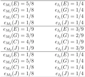
a uniform probability distribution. The final emission probabilities can be seen in Table 4.

The next step involves calculating the transition probabilities. In this step we use the following formula in 2 to calculate the probabilities.

Table 4: Emission Probabilities for the MSA in Table 3 𝑒𝑀1(𝐸) = 5/8 𝑒𝐼1(𝐸) = 1/4 𝑒𝑀1(𝐺) = 1/8 𝑒𝐼1(𝐺) = 1/4 𝑒𝑀1(𝐶) = 1/8 𝑒𝐼1(𝐶) = 1/4 𝑒𝑀1(𝐽) = 1/8 𝑒𝐼1(𝐽) = 1/4 𝑒𝑀2(𝐸) = 1/9 𝑒𝐼2(𝐸) = 3/9 𝑒𝑀2(𝐺) = 3/9 𝑒𝐼2(𝐺) = 2/9 𝑒𝑀2(𝐶) = 4/9 𝑒𝐼2(𝐶) = 1/9 𝑒𝑀2(𝐽) = 1/9 𝑒𝐼2(𝐽) = 3/9 𝑒𝑀3(𝐸) = 1/8 𝑒𝐼3(𝐸) = 1/4 𝑒𝑀3(𝐺) = 5/8 𝑒𝐼3(𝐺) = 1/4 𝑒𝑀3(𝐶) = 1/8 𝑒𝐼3(𝐶) = 1/4 𝑒𝑀3(𝐽) = 1/8 𝑒𝐼3(𝐽) = 1/4

Similar to the case of the emission transition probabilities we use the add one rule to remove the zero probabilities. Calculating the transition probabilities from the begin state B to 𝑀1 state we get 𝑎𝐵𝑀1 = 4/5. And the transition probabilities from the

begin state B to insert state 𝐼0 and delete state𝐷1 are 𝑎𝐵𝐷1 = 1/5 and 𝑎𝐵𝐷1 = 1/5

For the add one-one rule we add one to the numerator and the total number of possible transitions that is three to the denominator. Hence after the add one rule we get

𝑎𝐵𝑀1 = (4 + 1)/(5 + 3) = 5/8, 𝑎𝐵𝐷1 = 2/8, and 𝑎𝐵𝐼0 = 1/8.

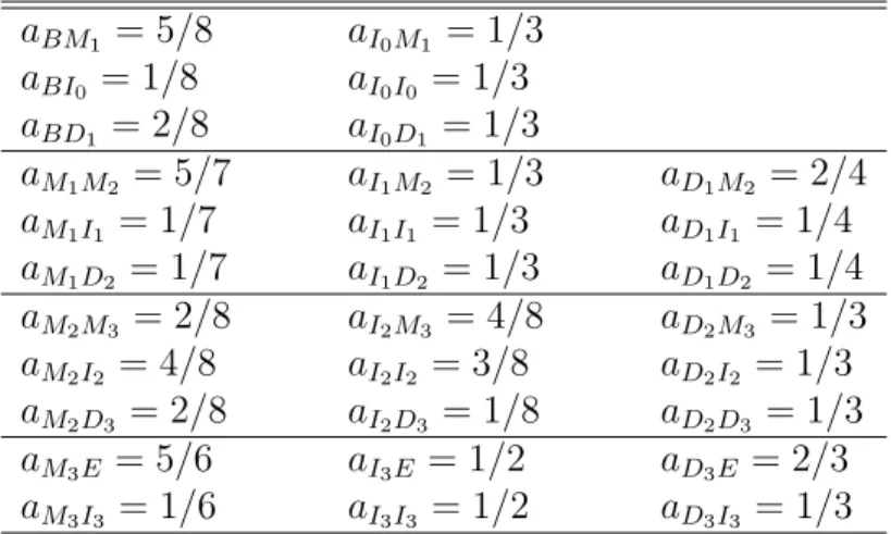
For the states which we have no data we assume a uniform distribution and assign a value of 1/3. Using this method we compute all the values and the results are shown in table 5.

We have now successfully constructed the PHMM from the MSA and the next step is scoring. Similar to the case of the HMM the algorithm used for scoring is the forward algorithm. The target of the algorithm is to compute the score of a given

Table 5: Transition Probabilities for the MSA in Table 3 𝑎𝐵𝑀1 = 5/8 𝑎𝐼0𝑀1 = 1/3 𝑎𝐵𝐼0 = 1/8 𝑎𝐼0𝐼0 = 1/3 𝑎𝐵𝐷1 = 2/8 𝑎𝐼0𝐷1 = 1/3 𝑎𝑀1𝑀2 = 5/7 𝑎𝐼1𝑀2 = 1/3 𝑎𝐷1𝑀2 = 2/4 𝑎𝑀1𝐼1 = 1/7 𝑎𝐼1𝐼1 = 1/3 𝑎𝐷1𝐼1 = 1/4 𝑎𝑀1𝐷2 = 1/7 𝑎𝐼1𝐷2 = 1/3 𝑎𝐷1𝐷2 = 1/4 𝑎𝑀2𝑀3 = 2/8 𝑎𝐼2𝑀3 = 4/8 𝑎𝐷2𝑀3 = 1/3 𝑎𝑀2𝐼2 = 4/8 𝑎𝐼2𝐼2 = 3/8 𝑎𝐷2𝐼2 = 1/3 𝑎𝑀2𝐷3 = 2/8 𝑎𝐼2𝐷3 = 1/8 𝑎𝐷2𝐷3 = 1/3 𝑎𝑀3𝐸 = 5/6 𝑎𝐼3𝐸 = 1/2 𝑎𝐷3𝐸 = 2/3 𝑎𝑀3𝐼3 = 1/6 𝑎𝐼3𝐼3 = 1/2 𝑎𝐷3𝐼3 = 1/3

sequence X = 𝑥1, 𝑥2,. . . ,𝑥𝑛 of length 𝐿 with (𝑁 + 1) states based on how well it matches with the PHMM model. State 0 and state 𝑁 are the begin and end states respectively. The forward algorithm computes the probability of a a given sequence in the PHMM model recursively. Hence it is a very efficient algorithm. Below of all the recursive relations are described [23].

𝐹_𝑗𝑀(𝑖) = log (︂_𝑒 𝑀𝑗(𝑥𝑖) 𝑞𝑥𝑖 )︂ + log (︁ 𝑎𝑀𝑗−1𝑀𝑗exp (︀ 𝐹_𝑗𝑀−1(𝑖−1) )︀ +𝑎𝐼𝑗−1𝑀𝑗exp (︀ 𝐹_𝑗𝐼₋₁(𝑖−1))︀ +𝑎𝐷𝑗−1𝑀𝑗exp (︀ 𝐹_𝑗𝐷₋₁(𝑖−1))︀)︁ 𝐹_𝑗𝐼(𝑖) = log (︂_𝑒 𝐼𝑗(𝑥𝑖) 𝑞𝑥𝑖 )︂ + log(︁𝑎𝑀𝑗𝐼𝑗exp (︀ 𝐹_𝑗𝑀(𝑖−1))︀ +𝑎𝐼𝑗𝐼𝑗exp (︀ 𝐹_𝑗𝐼(𝑖−1))︀ +𝑎𝐷𝑗𝐼𝑗exp (︀ 𝐹_𝑗𝐷(𝑖−1))︀ )︁ 𝐹_𝑗𝐷(𝑖) = log(︁𝑎𝑀𝑗−1𝐷𝑗exp (︀ 𝐹_𝑗𝑀₋₁(𝑖))︀ +𝑎𝐼𝑗−1𝐷𝑗exp (︀ 𝐹_𝑗𝐼₋₁(𝑖))︀ +𝑎𝐷𝑗−1𝐷𝑗exp (︀ 𝐹_𝑗𝐷₋₁(𝑖))︀)︁

The value for the base case for this algorithm is zero and 𝑞𝑥𝑖 is the distribution of𝑥𝑖. From the forward algorithm all the terms provide the score of a given sequence and the sum of the scores provides the final score. In order to be able to compare scores for different sequences directly we normalize the score by dividing it by the length of the sequence. The logarithms take care of any possible underflow problems. In [3] an in depth analysis has been done in using the PHMM model for detecting computer virus variants generated using construction kits. The PHMM model was created using the opcode sequences. The experiments proved that the PHMM was able to achieve a high detection rate for the chosen malware families. The work also shows that the PHMM based detection was successful in detecting even the hard to detect metamorphic viruses. The authors in [6] have also achieved good results using PHMM in aligning words that linguistically have the same root. Given the success of PHMM in various applications in this project we extend the work in [3] to perform

the PHMM based detection using dynamic analysis. The implementation details are discussed in Chapter 3.

2.6 Analysis Techniques

Software birthmarks are characteristics that are unique to a particular software. There are two types of birthmarks - static and dynamic Birthmarks. The static birth-marks are the characteristics that can be extracted from the program itself without executing it. For example opcodes sequences can be considered as a static birthmark for a program.

Dynamic birthmarks are the characteristics that are obtained from a program when it is executed. These can be API calls that are recorded when the program is executed.

In this section we will discuss two main analysis techniques which use the concept of static and dynamic birthmarks for malware Detection

2.6.1 Static Analysis

Static Analysis involves analyzing the program without executing it. In [21] static analysis is performed by extracting opcode sequences with the help of a disassembler. The key advantage of static analysis is that it is more efficient, fast and a more preferred approach if it works effectively as it is less expensive in terms of consuming the system resources. Compared to the dynamic analysis technique, it is also safer since it does not involve the execution of the malware. The drawback of this technique is that it can easily be defeated by simple code obfuscation techniques like morphing the virus, garbage code insertion or encrypting the virus [4].

2.6.2 Dynamic Analysis

Dynamic Analysis is performed by extracting dynamic software birthmarks. Dy-namic birthmarks, such as Application Program Interface(API) calls obtained at run-time, cannot be defeated so easily [31] and hence a powerful signature of a particular malware family for detection. Dynamic birthmarks are resilient to code obfuscation when compared to the static birthmarks. The disadvantages of dynamic analysis is that it is more expensive, can be potentially harmful as it involves executing the malware and is slower compared to static analysis.

In this project we use the dynamic and static birthmarks for malware detection. We compare the results obtained from dynamic and static analysis. We then attempt to show that the results obtained from dynamic analysis are better compared to static analysis in terms accuracy.

2.7 Previous Work

There has been a lot of research done in the field of static and dynamic birth-marks. In this section we will review some of the static and dynamic birthmark techniques.

2.7.1 𝐾-gram Based Techniques

In [18] the authors propose a static 𝑘-gram based birthmark. This birthmark is computed by extracting unique opcodes of length 𝑘 for a module. The effectiveness of this birthmark is tested on randomly selected applications and also on programs that are semantically different but accomplish the same task. The authors identify an optimum k value at which the credibility and resilience of the birthmark is maximized.

Continuing on this work the authors in [5] have proposed a dynamic birthmark based on the 𝐾-gram technique. In this paper the authors construct a 𝑘-gram based birthmark by traversing a window of length𝑘 over an opcode sequence in the case of static and over an executable trace for the case of dynamic. The authors evaluated the strength of the dynamic birthmarking technique by comparing the results obtained from static and dynamic cases when code obfuscation is applied. They show that the static 𝑘-gram birthmark fails with simple code obfuscation like insertion of dead code. On the other hand, dynamic 𝑘-gram birthmark is much more robust since it is based on runtime behavior which is tougher to change by an attacker.

2.7.2 Graph Based Technique

Another novel technique is discussed in [2]. This is a graph based technique in which a graph is constructed by collecting dynamic instruction traces of an executable file. The constructed graphs are Markov chains consisting of instructions and transi-tion probabilities. A similarity matrix is created using the graph kernels for different instruction traces. A Support Vector Machine takes this similarity matrix as input to perform the malware classification. The author shows that this technique is an improvement over raw 𝑛-gram, signature and machine learning based techniques.

2.7.3 API Calls Based Techniques

Next, we look at a birthmark technique discussed in [31]. In this paper two birthmarks are proposed which are the API call sequences and API call frequencies that are collected during runtime. As mentioned in the previous papers, altering information at runtime is very tough to accomplish by an attacker because it is difficult to substitute API calls with equivalent ones especially in the case of file

I/O, semaphore and GUIs APIs without altering program behavior. The authors leverage this fact for creating a strong dynamic birthmark. A key fact to note is that different programs using the same APIs will not have the same order of API calls upon execution. In the event that an attacker is able to alter the API call sequences, the frequency of API calls would remain unchanged. Hence the author looks at a combination of both the birthmarks discussed above to make the detection technique more robust.

2.7.4 Operand Stack Runtime Based Technique

In the papers above we have predominantly looked at API calls as dynamic birthmarks. In [12] the authors use the operand stack runtime behavior of a Java Virtual Machine. This is considered as a birthmark due to its unique nature at runtime. This birthmark exhibits high tolerance towards code change and good ability to discern programs that could be a pirated version of another.

It is evident from the works above that dynamic birthmarks have inherent ad-vantages over its static counter parts. Having done an extensive survey of existing research, our work is built upon idea of using a dynamic birthmark in the field of malware detection using machine learning based detection techniques.

CHAPTER 3 Implementation

This chapter consists of the method used in the implementation part of the project. The first section gives information about the training and testing approach using HMMs. The second section gives information on training and testing using PHMMs. The third section contains an overview of how the data was collected. The fourth section gives details about the tools used in the project

3.1 HMM

3.1.1 Dynamic Analysis Technique

In order to perform the dynamic analysis, we used the Buster Sandbox Analyzer to execute the malware and benign datasets and collected API call logs. Then we extracted the API calls from the log files by writing shell scripts. These constitute the dynamic birthmarks of the chosen malware. These API call sequences were then ap-pended to form a long observation sequence that was sent for training using the HMM. After the training step is completed a model is obtained from the HMM. This model is then used during the scoring step. The malware and benign sets are scored against the model. These scores are then plotted in a scatter plot. From the scatterplot the separation between the malware and benign scores were observed to determine the separation. Then the ROC curves were plotted to determine the effectiveness of the chosen birthmark and the area under the curve(AUC) was calculated.

The training was performed for 1000 to 1500 iterations depending on the chosen dataset till the 𝐵 matrix values converged completely. The five-fold cross-validation

divided the dataset into five groups. Four of the five groups were used for training and one group was used for testing. This process was performed five times until all the permutation of groups have been used for training and testing. We performed the experiments for seven different malware families. In our experiments we have chosen

𝑁 (number of hidden states)=2.

3.1.2 Static Analysis Technique

This technique Involves disassembling the malware using the IDA Pro disassem-bler. After which the opcode sequences are extracted from the malware. We then wrote scripts to extract only the opcodes and disregard the operands and the rest of the data. These constitute the static birthmarks of the chosen malware. The opcode sequences from all the files were merged to form a observation sequence which was then sent for training using the HMM. After the training step is completed a model is obtained from the HMM. The malware and benign set are scored against the model. We then created a scatterplot from the scores. From the scatterplot the separation between the malware and benign scores are observed and ROC curves are also plot-ted to determine the effectiveness of the chosen birthmark. Similar to the dynamic analysis technique, the training was performed for 1000 to 1500 iterations depending on the chosen dataset till the 𝐵 matrix values converged completely. The five-fold cross-validation method was also used in this case [14, 21] similar to the dynamic analysis case mentioned previously. In this case also we have chosen 𝑁=2 and we have performed the experiments on seven different malware families.

3.2 PHMM

The goal here is to create a MSA from the sequences of API calls that are obtained from the malware families and build a PHMM model from it. Using the PHMM model we will score the benign and malware sequences to test the effectiveness of this technique in the field of malware detection using dynamic analysis.

The first step involves preprocessing the input dataset for each malware fam-ily individually. This involves mapping the API call sequences to alphabet[A-Z], numbers[0-9] and the asterisk symbol "*" based on the frequency of occurrence. After this step we will have a total of 37 unique symbols. This preprocessing step simplifies the process of aligning the sequences. The next step involves creating a substitution matrix by assigning scores for different combination of alignment of symbols. Then we build the MSA using the pairwise alignment approach and dynamic programming taking into consideration the gap penalty functions using the approach in [3]. The algorithm used for building the MSA is the Feng-Dolittle algorithm. Given the MSA we next build the PHMM model from it using the implementation we have written. We developed a model for each of the families using a subset of the sequences. We have reserved the remaining sequences in the malware family for testing.

For building the PHMM model we did the following in our implementation. We first compute the begin probabilities. The begin states is considered to be the

𝑀0 state. The probabilities from 𝑀0 state to the first insert, match and delete

state are calculated. We then identify the match and insert states by identifying the conservative (columns which have more than half of the elements as deletes) and non-conservative columns. We then compute the emission probabilities by computing the frequency of symbols in each of the columns. The next step involves calculating

the columns. While performing the emission and transition probability calculations we use the add-one rule to avoid zero values that could overfit the data. Finally we calculate the end probabilities. The last state also known as the exit state is considered to be the 𝑀𝑛+1 state. The begin state and the exit state do not emit

symbols and hence we do not calculate the emission probabilities [3] for this case. Once we have built the PHMM model we then use the forward algorithm to compute scores against the PHMM model. The scoring program generated three different scores. They are scores of the input sequence ending in a insert, match or delete state. We then sum up the three values to get the final score. In order to be able to compare scores for different sequences we normalize the scores. We achieve this by dividing the final score with the length of the sequence. We have used malware sequences from the same family and benign sequences for the scoring. The details of the forward algorithm used are described in chapter2.

3.3 Chosen Dataset

For the Malware set we have considered seven different malware families:

Zbot: Zbot is a Trojan that compromises the system it infects and steals all the confidential information from the system such as online credentials [26].

Cridex: Cridex is a worm that multiplies and spreads through removable drives. It downloads malicious programs into the system it has attacked [25].

Winwebsec: Winwebsec is a Trojan that generally attacks users of windows op-erating systems. It impersonates anti-malware software and displays fake messages saying that the user’s system has been infected. It then makes the user pay for the fake anti-malware product to remove the threats [17].

SmartHdd: SmartHdd is a malware that targets users of Windows operating system. It tricks the users into thinking that it is SMART hardware monitoring system and hence the name. It generates fake messages indicating that the hard drive is failing and makes the user pay in order to fix the issue. It also disables the antivirus software in the compromised systems [13].

Security Shield: This is a fake antivirus software that falsely claims that it will protect the system from malware and demands the user to pay money to get the full version [16].

Zeroaccess: This is a Trojan that attacks systems with Windows operating sys-tem. It downloads other malicious programs into the compromised system from a botnet [29].

Harebot: This is a backdoor malware that generally affects the systems with Windows operating system. It brings down the productivity of the compromised system. It provides a backdoor for the hackers to gain access to the compromised system and steal information [19]. Table 6 has the list of malware families and number of files used in this project

Table 6: Benign files

Malware family Number of files

Zbot 100 Cridex 50 Winwebsec 100 SmartHdd 50 Security Shield 50 Zeroaccess 100 Harebot 50

dows 7 along with some freeware. Table 8 has the list of benign files used in this project

Table 7: Benign files

No. Benign file 1 bdaycontrol.exe 2 IRATrack.exe 3 MineSweeper.exe 4 SpiderSolitaire.exe 5 PurblePlace.exe 6 FreeCell.exe 7 Chess.exe 8 7zFM.exe 9 hh.exe 10 Mahjong.exe 11 DVDMaker.exe 12 datewiz.exe 13 winhlp32.exe 14 bdaycheck.exe 15 setup.exe 16 Countdown Pro.exe 17 unins000.exe 18 bckgzm.exe 19 nanoclock.exe 20 shvlzm.exe

3.4 Tools Used In the Project

3.4.1 Tools Used for Dynamic Analysis

For this project we used the Buster Sandboxie Analyzer(BSA) for getting the API calls. The BSA is an analyzer that analyzes malware behavior of processes. It captures all the changes made to the system by the processes. The information captured by the BSA include file system changes, windows registry changes and port changes. The sandbox software which is in this tool helps protect the system when

the malware is being executed. It prevents the malware from making changes into the system [9].

3.4.2 Tools Used for Static Analysis

The other tool that was used in the project was IDA Pro. IDA Pro is a disas-sembler which can generate machine level code given an executable file. This tool was used to disassemble the malware and benign set and generate the asm files. The opcodes were the extracted from these asm files with the help of scripts.

CHAPTER 4 Experiments and Results

The main goal of our experiments is to test the effectiveness of the dynamic analysis technique. This chapter comprises of the setup and the results of the exper-iments of the project. The setup section consists of the specifications of the host and the guest machines. The results section contains the discussion on the results of the project.

4.1 Setup

In this project, we have used a virtual machine container and we have taken the snapshots of the whole system for recovery purposes. We have used the Oracle VM Virtual Box. The host machine that we used had a Intel(R) Core(TM) i5-3317U [email protected] processor, 6GB RAM, 64-bit Operating system and Windows 8.1 operating system. The guest machine that we used in out experiments was a Oracle Virtual Box 4.3.16 VMs and it consisted of a base memory of 3310MB, 6 GB RAM, 32 bit operating system and Windows 7 operating system.

The training and testing of the HMMs and PHMM are done in the host machine whereas the API calls and opcode extraction are done in the guest machine.

4.2 Results

After performing the experiments we plotted Receiving Operating Characteristics (ROC) and calculated Area Under the Curve (AUC) for all the malware families.

4.2.1 Receiving Operating Characteristics

Receiving operating characteristic (ROC) is a graphical plot used to determine the effectiveness of a machine learning algorithm. In this project we will be using this as a bench marking tool for evaluating the performance of the machine learning techniques for our feature set. We construct the ROC by plotting the true positive rate (TPR) versus the False positive rate (FPR) by taking into consideration different thresholds. It can be seen in Figure 4 that there is a shaded region in the ROC curve. The Area Under the Curve is obtained by calculating the area in the shaded region. This value lies between 0.5 and 1. An AUC of 1 implies that it has no false positive or false negatives and can hence classify perfectly [22]. Figure 4 is an example of a ROC curve where the area under curve is 1. It has been show in [7] that ROC works efficiently as a classification performance measure for machine learning algorithms.

Figure 4: ROC Curve

4.2.2 Hidden Markov Model

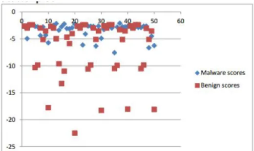
We perform HMM on seven malware families using both static and dynamic analysis. We then plot the ROC for each case and calculate the AUC. To perform a comparison on both the techniques we have chosen the same data set in both cases. We now consider a single family and examine the results. Figure 5 and A.13 show the

scatterplot and the ROC curve for the security shield malware family respectively.

Figure 5: Security Sheild: Scatterplot

Figure 6: Security Shield: Area Under the Curve

It can be seen that there is a clear separation between the malware and benign scores. The AUC = 1 for this family using dynamic analysis. This implies that it is a perfect classifier and does not not have any false positives or false negatives. This indicates that the dynamic analysis technique using HMM works effectively for detecting malware.They represent the scatterplot and the ROC curve for the security shield malware family respectively. We now turn our attention to the Figure 7 and B.20

Figure 8: Security Shield: Area Under the Curve.

It can be seen from the scatterplot that there is a lot of misclassification of the malware and benign files and there is no clear separation between the scores unlike in the dynamic analysis case. Also the AUC = 0.676 indicates that it is a very poor classifier. It can be clearly seen that dynamic analysis using HMM based de-tection has outperformed static analysis. We have performed experiments on a total of seven malware families and the scatterplots and ROC curves are presented in the appendix A for dynamic analysis and appendix B for static analysis. A summary of the results comparing the area under the curves obtained from static and dynamic analysis using HMM for all the malware families are presented in the Table 8. From the table we can see that the AUC for dynamic analysis is much greater the AUC for static analysis except for the case of the SmartHdd malware family where the static analysis has marginally performed better than dynamic analysis. This is be-cause the number of unique API calls obtained from SmartHdd were fewer in number compared to the unique opcodes in the static analysis case which makes the HMM model weaker for classifying malware and benign files. On an average the AUC for dynamic analysis technique is 0.976 the average AUC for the static analysis technique is 0.785. It clearly shows that the our dynamic analysis technique has outdone the static analysis technique and that our chosen birthmarks are effective in detecting malware. This is because the dynamic analysis requires the execution of the malware

which removes a layer of obfuscation and hence provides a robust birthmark for de-tecting malware. Also in the case of static analysis we just consider opcode sequences which do not capture the actual behavior of the malware. In the case of dynamic analysis we take into account the execution trace which is unique to different malware families at different inputs and hence captures the unique behavior of the malware and hence renders itself nicely as a dynamic birthmark. Although the dynamic anal-ysis technique is expensive as it involves executing the malware the classification is far better than static analysis.

Table 8: AUC curve results for static and Dynamic Analysis

AUC Malware family Dynamic Static

Zbot 0.990 0.847 Security Shield 1.000 0.676 Cridex 0.964 0.596 Zeroaccess 0.979 0.923 Winwebsec 0.985 0.835 SmartHdd 0.980 0.996 Harebot 0.974 0.622

4.2.3 Profile Hidden Markov Model

In the previous section we discussed we have seen that the HMM technique using dynamic analysis has performed well. In this section we test the effectiveness of the PHMM technique to see if we can get improved scores over the HMM technique in the field of malware detection using the dynamic analysis approach. We have achieved this by considering each malware family individually and then grouping the sequences in increments of 5 or 10 sequences. We have then created the PHMM model for each of these groups. We have done this to check which grouping of sequences produces

effective results. We have kept the mapping used for the malware families fixed for the scoring involved for the respective malware families. For scoring we have used benign sequences and unseen malware sequences of the family. The score of a sequence with respect to the model will give the similarity of the sequence to the model. A high score indicated that the sequences is related to the model and a low score indicated that it is not similar.

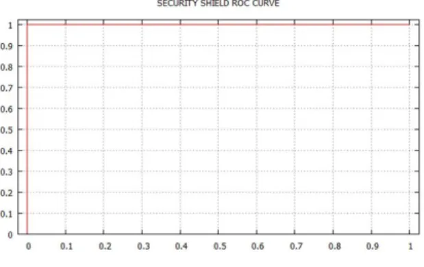
The ROC curves obtained using PHMM for all the possible groups for the ze-roaccess family if provided in figure C.30. It can be seen that we get an AUC of 1 for groups 30, 50 and 70 and for the remaining groups the AUC is above 0.90. This implies that we are able to get a group for which we get perfect classification.

Figure 9: Zeroaccess PHMM ROC -all groups

We have performed the experiments for all the malware families for different grouping of sequences. And the summary of the results are provided in Table 9. The ROC Curves for all the families are presented in Appendix C

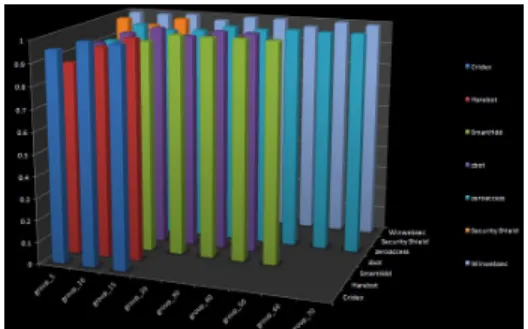
Figure 10 shows a graphical representation of the AUC obtained for all groups of the malware families using PHMM.

Figure 10: PHMM results -all groups

We select the maximum AUC value among all the groups for each of the mal-ware family and that will represent the AUC for that particular malmal-ware family. To compare the performance of the PHMM over the HMM technique we have plotted a bar graph considering the AUC for each malware family in Figure 11. It can be seen that PHMM has performed consistently well across all the families with an AUC of 1. This implies that we are able to achieve perfect detection using PHMM consistently. This is because we are taking into account the positional information of the sequences and it provides more information of the malware’s behavior. The HMM technique using dynamic analysis has also performed comparatively well with the minimum AUC being 0.96 and maximum AUC being 1 for Security shield. This shows that the chosen dynamic birthmark is able to capture the behavior of the malware effectively and is effective for malware detection.

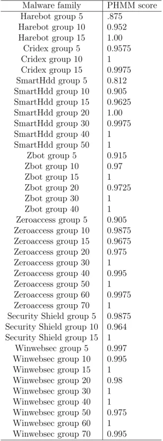
Table 9: PHMM Results

Malware family PHMM score Harebot group 5 .875 Harebot group 10 0.952 Harebot group 15 1.00 Cridex group 5 0.9575 Cridex group 10 1 Cridex group 15 0.9975 SmartHdd group 5 0.812 SmartHdd group 10 0.905 SmartHdd group 15 0.9625 SmartHdd group 20 1.00 SmartHdd group 30 0.9975 SmartHdd group 40 1 SmartHdd group 50 1 Zbot group 5 0.915 Zbot group 10 0.97 Zbot group 15 1 Zbot group 20 0.9725 Zbot group 30 1 Zbot group 40 1 Zeroaccess group 5 0.905 Zeroaccess group 10 0.9875 Zeroaccess group 15 0.9675 Zeroaccess group 20 0.975 Zeroaccess group 30 1 Zeroaccess group 40 0.995 Zeroaccess group 50 1 Zeroaccess group 60 0.9975 Zeroaccess group 70 1 Security Shield group 5 0.9875 Security Shield group 10 0.964 Security Shield group 15 1

Winwebsec group 5 0.997 Winwebsec group 10 0.995 Winwebsec group 15 1 Winwebsec group 20 0.98 Winwebsec group 30 1 Winwebsec group 40 1 Winwebsec group 50 0.975

CHAPTER 5

Conclusion and Future work

Growing malware and cyber threats have necessitated the need for robust and efficient detection techniques. In our project we analyzed the static and dynamic antivirus detection techniques and identified the advantages of dynamic analysis. We then applied the dynamic analysis techniques for malware detection using the Hidden Markov Model and Profile Hidden Markov Model machine learning techniques.

HMM has been proven to be successful in the field speech recognition, software piracy detection and metamorphic malware detection [14, 21]. Given that it is a popular machine learning technique with good rates of success we have chosen to implement HMM to detect malware using the dynamic analysis technique.

For the dynamic analysis technique we extracted the API calls from the malware and benign files. We then tested to see if the HMM technique is effective in detecting malware using dynamic analysis. Our results show that the HMM technique using dynamic analysis is robust in detecting malware. In order to get an idea on how the dynamic analysis technique performed over static analysis we performed static analysis on the same malware families. Our results show that the dynamic analysis has out performed static analysis. This is because of the fact that the dynamic analysis technique removes a layer of obfuscation and hence provides a more effective way of detecting malware. The average AUC we obtained for all the families using dynamic analysis was 0.976 and the average AUC we obtained for all the families using static analysis was 0.785. We were able to prove that the dynamic analysis using HMM is better than static analysis and that our chosen dynamic birthmark is

effective in detecting malware.

In our project we have also implemented the PHMM in the field of malware detection. PHMM has been successful in the field of bio informatics and works well in identifying the relation between DNA sequences. Given that PHMM works well with sequences it lends itself nicely for malware detection using dynamic analysis. We have tested our PHMM model for different grouping of sequences and we were able to a achieve perfect detection for all the malware families. This shows that the PHMM model along with the chosen dynamic birthmark is able to capture the behavior of the malware family effectively and is effective in malware detection.

For future work, these experiments can be extended to metamorphic viruses where the HMM and PHMM technique can be performed at different morphing ra-tios using the dynamic analysis approach to test its effectiveness. The performance of dynamic analysis can be compared with the static analysis technique to determine which technique works the best for metamorphic viruses. The dynamic birthmark considered in this paper are API calls. The dynamic analysis approach can be tried for different birthmarks and a more efficient birthmark can be identified. Another potential approach can be combining the API calls with other types of dynamic birth-mark using a Support Vector Machines to develop an even robust malware detection model. The effectiveness of dynamic analysis can be tested by applying advanced code obfuscation technique to the malware hence providing a challenging dataset for testing. Different machine learning based detection techniques can be applied using dynamic analysis to evaluate the performance of dynamic analysis for different cases. .

LIST OF REFERENCES

[1] C. Annachhatre, M. Stamp, T. Austin Hidden Markov Models for Malware Clas-sification,Journal of Computer Virology and Hacking Techniques,2014

[2] B. Anderson, Graph-Based Malware Detection Using Dynamic Analysis. Journal in Computer Virology,7(4) 247-258 (2011)

[3] S. Attaluri, S. McGhee, M. Stamp, Profile Hidden Markov Models and Meta-morphic Virus Detection, Journal in Computer Virology, 5(2):151–169, 2009 [4] J. Aycock,Computer Viruses and Malware, Springer, 2006

[5] Y. Bai, X. Sun, G. Sun, X. Deng, X. Zhou,Dynamic K-Gram Based Software Birthmark,19th Australian Conference on Software Engineering,2008

[6] A. Bhargava, G. Kondrak, Multiple Word Alignment with Profile Hidden Markov Models, In Proceedings of Human Language Technologies: The 2009 Annual Conference of the North American Chapter of the Association for Computational Linguistics, Companion Volume: Student Research Workshop and Doctoral Con-sortium, pp. 43–48, June, Boulder, Colorado

[7] A. P. Bradley, The Use of the Area Under the ROC Curve in the Evaluation of Machine Learning Algorithms, Journal Pattern Recognition, 30(7):1145–1159, 1997

[8] Symmantec(2010), Back Orifice

http://www.symantec.com/avcenter/warn/backorifice.html

[9] Buster Sandboxie Analyzer(2014)

http://bsa.isoftware.nl/

[10] CNN Money(2013),Target credit card hack: What you need to know

http://money.cnn.com/2013/12/22/news/companies/target-credit-card-hack/

[11] eWeek(2014),Twitter Resets 250,000 User Passwords After Cyber-Attack

http://www.eweek.com/security/twitter-resets-250000-user-passwords-after-cyber-attack/

[12] K. Fukuda, H. Tamada, A Dynamic Birthmark from Analyzing Operand Stack Runtime Behavior to Detect Copied Software, in Proceedings of 14th Interna-tional Conference on Software Engineering, Artificial Intelligence, Networking