Eigenvalue Analysis for Metamorphic Detection

San Jose State University

SJSU ScholarWorks

Master's Projects Master's Theses and Graduate Research

Fall 2012

Eigenvalue Analysis for Metamorphic Detection

Sayali Deshpande

Follow this and additional works at:https://scholarworks.sjsu.edu/etd_projects Part of theComputer Sciences Commons

This Master's Project is brought to you for free and open access by the Master's Theses and Graduate Research at SJSU ScholarWorks. It has been Recommended Citation

Deshpande, Sayali, "Eigenvalue Analysis for Metamorphic Detection" (2012).Master's Projects. 279. DOI: https://doi.org/10.31979/etd.33h5-kqrg

Eigenvalue Analysis for Metamorphic Detection

A Project Presented to

The Faculty of the Department of Computer Science San Jose State University

In Partial Fulfillment

of the Requirements for the Degree Master of Science

c

2012

The Designated Project Committee Approves the Project Titled

Eigenvalue Analysis for Metamorphic Detection

by

Sayali Deshpande

APPROVED FOR THE DEPARTMENTS OF COMPUTER SCIENCE

SAN JOSE STATE UNIVERSITY

December 2012

Dr. Mark Stamp Department of Computer Science Dr. Richard Low Department of Mathematics Dr. Sami Khuri Department of Computer Science

ABSTRACT

Eigenvalue Analysis for Metamorphic Detection by Sayali Deshpande

Metamorphic viruses change their structure on each infection while maintaining their function. Although many detection techniques have been proposed, practical and effective metamorphic detection remains a difficult challenge.

In this project, we analyze a novel method for detecting metamorphic viruses. Our approach was inspired by a well-known facial recognition technique that is based on eigenvalue analysis. We compute eigenvectors using opcode sequences extracted from a set of known metamorphic viruses. These eigenvectors can then be used to score a given executable file, based on its extracted opcode sequence. We perform extensive testing to determine the effectiveness of this scoring technique for classifying metamorphic malware. Our results show that this approach yields very good results when applied to highly metamorphic malware.

ACKNOWLEDGMENTS

I would like to thank my project advisor Dr. Mark Stamp for his encouragement, guidance and support throughout this project. I would also like to express my sincere gratitude to the committee members Dr. Richard Low and Dr. Sami Khuri for their time and patience. Special thanks to Dr. Wasin So for helping us out with difficult mathematical part in this project.

I am grateful to both Lisa Manning and Leesa Stanion for their scrupulous re-view of the text and valuable editing inputs. Finally, I wish to thank my husband Mr. Sushant Paithane for his unending patience and guidance throughout my Masters.

TABLE OF CONTENTS

CHAPTER

1 Introduction . . . 1

2 Simple to Metamorphic Virus . . . 3

2.1 Metamorphic Techniques . . . 4

2.1.1 Instruction Reordering . . . 5

2.1.2 Garbage Code Insertion . . . 5

2.1.3 Instruction Substitution . . . 5

2.1.4 Register Swapping . . . 5

2.1.5 Host Code Mutation . . . 6

2.1.6 Code Integration . . . 6

2.2 Examples of Metamorphic Viruses . . . 6

2.2.1 G2 . . . 6

2.2.2 MPCGEN . . . 6

2.2.3 NGVCK . . . 7

2.2.4 MWOR . . . 7

3 Metamorphic Virus Detection Techniques . . . 8

3.1 Wildcard string scanning . . . 8

3.2 Code Disassembling . . . 9

3.3 Code Emulation . . . 9

3.4 Heuristic-based Recognition . . . 9

3.6 Hidden Markov Models . . . 10

4 Eigenfaces . . . 11

4.1 Eigenvalue and Eigenvectors . . . 12

4.2 Image Detection . . . 13 5 Eigenviruses . . . 17 5.1 Algorithm . . . 17 5.1.1 Training Set . . . 17 5.1.2 Test set . . . 20 6 Implementation . . . 21 6.1 Opcode Extraction . . . 21 6.2 Normalization . . . 21 6.3 Virus Detection . . . 22 6.4 Setup . . . 23 7 Experimental Results . . . 24 7.1 Results . . . 24 7.1.1 G2 . . . 25 7.1.2 MPCGEN . . . 25 7.1.3 NGVCK . . . 26 7.1.4 MWOR . . . 26

7.2 Results for MWOR binaries . . . 27

8 Conclusion . . . 34

8.1 Future work . . . 35

APPENDIX A Opcode to Bytecode Map . . . 38

B Additional Graphs . . . 42

B.1 Euclidean distance Graphs . . . 42

B.1.1 MWOR with consolidated training set . . . 42

B.1.2 MWOR with different training sets . . . 42

B.1.3 MWOR with 20% eigenvectors . . . 43

B.1.4 MWOR with 6% eigenvectors . . . 43

B.1.5 NGVCK with 20% eigenvectors . . . 43

B.1.6 NGVCK with 6% eigenvectors . . . 44

B.2 ROC Graphs . . . 46

B.2.1 ROC for MWOR with 20% eigenvectors . . . 46

B.2.2 ROC for MWOR with 6% eigenvectors . . . 46

B.2.3 ROC for MWOR Binary files . . . 47

B.2.4 ROC for NGVCK with 20% eigenvectors . . . 47

B.2.5 ROC for NGVCK with 6% eigenvectors . . . 48

LIST OF TABLES

1 Experiment setup . . . 23

2 Virus families . . . 24

3 Benign Files . . . 24

4 AUC Statistics for virus families . . . 29

5 AUC Statistics for MWOR with training set of MWOR 0.5 . . . 30

6 AUC Statistics for MWOR binaries with training set of MWOR 0.5 . 31 7 AUC statistics for MWOR using HMM detection . . . 32

LIST OF FIGURES

1 Simple Virus Replication . . . 3

2 Encrypted Virus Replication . . . 3

3 Polymorphic Virus Replication . . . 4

4 Metamorphic Virus Replication . . . 4

5 Eigenvector . . . 13

6 Face Images [14] . . . 14

7 Eigenvectors from Face Images [14] . . . 15

8 Original and projected known image [14] . . . 16

9 Original and projected unknown image [14] . . . 16

10 Implementation . . . 22

11 G2 virus . . . 25

12 MPCGEN virus . . . 26

13 NGVCK virus . . . 27

14 MWOR opcodes with training set MWOR 0.5 . . . 28

15 MWOR binaries with training set MWOR 0.5 . . . 28

16 ROC for MWOR . . . 30

17 ROC for NGVCK . . . 31

18 ROC for MPCGEN . . . 32

CHAPTER 1 Introduction

With the advent of the internet and a plethora of devices ever-connected online, security is now an issue of paramount importance. Computer malware is a piece of software that can steal confidential information, compromise infected computer systems to perform any actions on behalf of a hacker, and can render computer systems unusable. Malware includes all families of viruses including computer worms, Trojans, rootkits, spywares, etc. Viruses can replicate and distribute themselves across a network. They can also have a catastrophic impact on corporate as well as individual computer systems [19].

A metamorphic virus can mutate itself at each infection such that each copy is different from the other but essentially performs the same malicious actions. Such viruses employ various techniques to change and obfuscate virus body such as in-struction reordering, garbage code insertion, register swapping, and so on. These mutations make it harder to detect metamorphic viruses.

Although many techniques have been proposed to detect metamorphic viruses, very few (if any) could operate as a commercial antivirus products. Recently, a novel approach was proposed for detection of metamorphic viruses that is based on a face-recognition technique called Eigenfaces [14]. Our technique for metamorphic virus detection is inspired by this approach. However, our technique differs from Eigenfaces in the way that it uses opcode sequences of virus files instead of raw

of operands. Our technique performs pre-processing on raw binary files and extracts opcodes in intermediate files. It implements the Eigenviruses algorithm and processes the opcode files for both the virus training set and the test set. The technique is extensively tested using four different highly metamorphic viruses. The results are analyzed and presented via AUC tables and ROC graphs. Results of the technique are then compared to the results of other metamorphic virus detection techniques such as HMM [18] technique and the Eigenviruses [11] technique which uses raw binary files.

This report is organized as follows. Section 2 provides an overview of metamor-phic viruses. Section 3 describes various metamormetamor-phic virus detection techniques. Section 4 briefly explains the face-recognition technique called Eigenfaces. Section 5 provides details of Eigenviruses metamorphic detection technique followed by our im-plementation in Section 6. Various test cases and results are discussed in Section 7. The report ends with the conclusion and suggests future enhancements.

CHAPTER 2

Simple to Metamorphic Virus

A computer virus is a program that infects host files and spreads the infection from one file to another much like a biological virus [8]. Simple virus replication can be illustrated as shown in Figure 1. These viruses can be detected using simple signature-based methods.

Figure 1: Simple Virus Replication

Second generation encrypted viruses carried their own decryptor attached to the virus body. The decryptor can create a slightly different copy of the virus at each infection. Encrypted viruses are able to evade signature-based detection. This can be illustrated in the following Figure 2.

body encrypted, these viruses could not be detected by signature detection. These are called Polymorphic viruses.

Figure 3: Polymorphic Virus Replication

More advanced metamorphic viruses can mutate their virus body at each new infection while maintaining their behavior. This does not require encryption because each new copy of the virus infects anew each time, and hence, signature-based detec-tion cannot be used. This property makes metamorphic viruses one of the hardest to detect among all the virus families.

Figure 4: Metamorphic Virus Replication

2.1 Metamorphic Techniques

There are many techniques used to generate metamorphic viruses. It is important to know these techniques in order to detect the viruses effectively. The following section describes some of these techniques.

2.1.1 Instruction Reordering

In this technique, virus code is divided among blocks of certain size. The muta-tion engine reorders these blocks of code producing different copy of the same virus. These different blocks are connected by inserting jump instructions to ensure the functionality of the program remains constant.

2.1.2 Garbage Code Insertion

Garbage Code Insertion is also called trash insertion or dead code insertion [11]. In this technique, a mutation engine inserts unnecessary code into the main body of the virus at random locations. The dead code does not serve any purpose in the main functionality of the virus. However, its important role is to obfuscate the body of the virus.

2.1.3 Instruction Substitution

With Instruction Substitution, certain instructions in the virus code are replaced by equivalent instructions that keep the functionality the same. This technique is used in metaphor mutation engines [11].

2.1.4 Register Swapping

As the name suggests, Register Swapping uses different registers to store operands of the virus instruction. Though it changes the appearance of the code it does not give high variability. This type of virus can be detected using a variant of signature based detection technique.

2.1.5 Host Code Mutation

Some viruses like Win95/Bistro mutate their own code as well as the code of the host file to which they attach [8]. A randomly executing code morphing routine is used to generate different copies of a virus. The code morphing routine can use several morphing techniques discussed above.

2.1.6 Code Integration

More advanced viruses such as Zmist, can decompose the host file into smaller elements and can insert itself into the code. Code Integration then rebuilds the code and also generates its references [8]. This way the virus integrates itself seamlessly into the host file, making it hard to detect or even repair.

2.2 Examples of Metamorphic Viruses

The following sub-sections briefly explain different metamorphic viruses.

2.2.1 G2

G2 is a second generation metamorphic virus generated by the G2 construction kit. It produces executable instances of G2 virus. The kit uses a configuration file to create virus files with desired features. It mainly uses the Instruction substitution technique to morph the virus code [11].

2.2.2 MPCGEN

This Mass Produced Code generation kit produces different copies of a virus. However copies exhibit more than 60% of similarity between them [4].

2.2.3 NGVCK

The Next Generation Virus Kit (NGVCK) uses code reordering, garbage code insertion and register swapping techniques to create highly metamorphic virus code. The virus creator engine is written in Visual basic and generates 32-bit executable files [11].

2.2.4 MWOR

MWOR is a metamorphic worm that carries its own engine. The engine’s body also mutates along with the virus code. It uses multiple morphing techniques such as garbage code insertion and instruction substitution [17].

CHAPTER 3

Metamorphic Virus Detection Techniques

Recent studies on computer viruses have focus on many new approaches for virus detection [18] [11] [2]. Some of them are purely academic and/or experimental techniques, while a few are being used in commercial antivirus products [11] . Meta-morphic virus detection is an active area of research due to its challenging nature and relevance to today’s cybersecurity concerns.

Daoud, Jebril et. al. in their paper ‘Computer Virus Strategies and Detection Methods’ [5] performed a calculated analysis of available metamorphic detection tech-niques. Based on their results they proposed the need for a newer and more efficient detection technique that can handle highly metamorphic viruses [5]. Their paper describes various computer virus strategies and detection methods and their known problems. Considering the complex nature of metamorphic viruses, it is critical to consider more innovative virus detection techniques that focus on the behavior of virus files along with their structural changes. Following are some of the methods used to detect metamorphic viruses.

3.1 Wildcard string scanning

Metamorphic viruses that use register swapping or instruction substitution meth-ods to generate virus copies, can be detected using Wildcard string scanning [9]. These virus files contain a common set of opcodes across various generations that can be extracted and matched to check for similarity between virus files.

3.2 Code Disassembling

By examining each instruction of the virus code, any garbage instructions can be identified. When this technique is used with a state machine model such as the Hidden Markov Model [18], this is a powerful tool for detecting viruses that use a dead code insertion technique [20].

3.3 Code Emulation

This technique requires a virtual machine to execute malicious code [8]. The virtual execution is monitored frequently to determine when interesting instruction is executed. The virus code cannot escape from a virtual machine.

3.4 Heuristic-based Recognition

This method is often employed to detect previously unknown viruses. Depending on features and behaviors of virus files, general rules are created to identify a suspi-cious file. However, this method is prone to false positive rates in case of metamorphic virus replication [9].

3.5 Geometric Detection

This method is based on a heuristic that attempts to evaluate how much the target victim file is changed from its original structure upon infection. It focuses on physical changes such as file size after infection. However, this method generates more false positives as the result of changes that may appear because of some unrelated activities [9].

3.6 Hidden Markov Models

This experimental research method uses the Hidden Markov Model (HMM) to detect metamorphic viruses [18]. The HMM model uses virus characteristics for training. In this technique, different copies of virus files become states of HMM and the opcode sequences are characterized as observations. This can be effective in identifying different viruses from the same virus family.

CHAPTER 4 Eigenfaces

In this section, we focus on yet another approach to effectively detect metamor-phic virus. According to the latest paper ‘Eigenviruses for Metamormetamor-phic Detection’ [11], a well known facial recognition technique called Eigenfaces can be used for metamorphic detection. Our metamorphic detection technique is motivated by this approach. Following sub-sections explain this technique in detail.

A computational model of face recognition can be quite complex and difficult when each and every feature of a face is considered in the process. It usually requires three-dimensional geometric computations [14]. However, when a face is assumed to be an upright flat image, it can be described by a smaller set of 2-dimensional vectors. This assumption helps in developing a face-recognition technique that is fast, simple and effective.

With this approach, face images are decomposed into small sets of characteristic feature images called ‘Eigenfaces’ [14]. These eigenfaces correspond to significant features of a face, but do not necessarily include intuitive features such as eyes, lips, nose, etc. The space spanned across eigenfaces is called ‘face-space’ [14]. When known and unknown face images are projected in this eigenspace, the euclidean distance between them can be used to determine if a new face is similar to a known face in the database [14].

unknown face images are represented in the same encoding. Finally, we compare the encoding results for both known and unknown images to determine if a new face matches to one in the database.

4.1 Eigenvalue and Eigenvectors

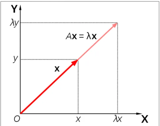
The words Eigenvalue and Eigenvectors are derived from the German word Eigen, which means ‘proper’ or ‘characteristic’ [6]. In linear algebra, if a non-zero vectorx

satisfies the following equation for matrix A, it is called an eigenvector ofA and λ is called the eigenvalue associated with the eigenvector x.

Ax=λx where,λ is a scalar

Figure 5 shows vector x and its transformation λx. If matrix A represents a transformation performed on vector x, then the resultant vector is a scalar multiple of the original vector x.

The variation between different images of faces can be thought as a transfor-mation from its eigenvector. This variation between different random data points is represented by a Covariance matrix [14]. In order to quantify similarity between different images, we would like to find eigenvectors of a covariance matrix. Each eigenvector is associated with its eigenvalue. The higher the eigenvalue, the more important the eigenvector is considered in the process. A higher eigenvalue means that its corresponding eigenvector accounts for the most variance within a set of face images [14].

Figure 6 shows the original face images used in computing a training set and Figure 7 displays the corresponding eigenvectors.

Figure 5: Eigenvector

4.2 Image Detection

When eigenvectors of the covariance matrix are drawn into a space, they enclose some area which is called eigenspace or face-space [11]. When a known image is projected onto a face-space, it can re-construct an image in terms of its eigenvectors as shown in Figure 8. When an unknown image is projected into the same eigenspace, the results may be radically different than expected. This is depicted in Figure 9.

An individual face image can be represented as a linear combination of the eigen-vectors. This corresponds to the small set of weights associated with each face image. Example: Suppose V denotes a vector which contains face image data.

Figure 6: Face Images [14] the following is true [14].

V =x1E1+x2E2+x3E3+. . .+x7.E7

where, x1, x2, . . . , .x7 denote the weights associated with vector V with respect to

eigenspace created by eigenvectors E1, E2, E3,. . . ,E7.

When these weights for known and unknown images are compared, we can infer whether the new image belongs to the training set.

Figure 8: Original and projected known image [14]

CHAPTER 5 Eigenviruses

The face-recognition scheme discussed in Section 4 is a reasonably simple and effective method for classifying and recognizing face images. In paper [11], analogous method is proposed that makes use of eigenvectors to quantify similarity between known and unknown virus files [11]. Our implementation of the detection technique is motivated from the method in paper [11]. However, our approach is significantly different in the sense that we use opcode instructions of virus files instead of raw binary files. We believe this approach is more effective because we focus on relevant information in the virus files while ignoring extraneous operand data.

In the following sections, we present the algorithm for metamorphic detection based on eigenviruses technique.

5.1 Algorithm

The following subsections explain the algorithm used to create the training sets from virus files.

5.1.1 Training Set

1. Acquire initial set of M virus files.

4. In order to quantify variation between different data points among all files, compute covariance matrix C for all vector files.

C = 1 M M X i=1 φiφTi (1) =AAT

where, M = number of files , A= [Φ1,Φ2,Φ3, ...,ΦM].

5. Ideally, we want to find eigenvectorsuof covariance matrixC, whereC =AAT. However, C is a N ×N matrix, which could be inefficient to compute. It can be shown that a matrix L, such that L = ATA , where L is M ×M matrix, can be used to find eigenvectors of C as follows:

Let vi be an eigenvector of matrix L. Then according to definition of

eigenvec-tors,

Lvi =λivi (2)

ATAvi =λivi whereλi is the eigenvalue,

Multiplying both sides byA, we get,

AATAvi =λiAvi (3)

i.e. CAvi =λiAvi

However, C = AAT _{and Av}

i is an eigenvector of matrix C. As a result, if v

is a set of eigenvectors of matrix L, where v = v1, v2..vi, then Av is a set of

6. Sort the set of eigenvectors u=u1, u2, ..uM according to their associated

eigen-valueλ. The magnitude of eigenvector is defined by eigenvalue. The higher the eigenvalue, the more important the eigenvector becomes as it can span across maximum characteristic features of original vectors.

7. We can then choose largest eigenvectors M0, where M0 < M. If we draw these eigenvectors into space, the enclosed area is called eigenspace. Here, we can ignore eigenvectors with smaller eigenvalues as they do not contribute in defining the boundary of the eigenspace.

8. The basic eigenspace we computed in the previous step is used to determine how much the original vector deviates from eigenspace. When these eigenvectors are linearly combined with specific weights it can give one of the original file vectors. Then, for file vectorφ and eigenvectors u1, u2, . . . , uM,

φ =u1ω1 +u2ω2+. . .+uMωM (4)

where, M = number of important eigenvectors i.e. φ= M X i=1 uiωi (5) then, ωi = M X i=1 uT_i φ (6)

The weights for virus file φi can be given as follows:

9. In this way, we calculate weight vectors for all virus files M and combine it into matrix ∆ as follows.

∆ = [Ω1,Ω2,Ω3, . . . ,ΩM] (8)

This becomes the training set for our technique.

5.1.2 Test set

We calculate weight vectors for the test files same as we did with training files as mentioned in Section 5.1.1. If the test files belong to the same virus family, their location in eigenspace would be closer to each other. In other words, the distance between the weight vectors of known and unknown files will be relatively short.

1. Project the input file Φk into eigenspace and determine its weights. ωi = M X i=1 uT_i φk (9) ΩT_k = [ω1, ω2, . . . , ωM] (10)

2. Compute Euclidean distance between weight vector of test file and each weight vector in the training set. If Ωi is weight vector from training set then the

euclidean distance between Ωk and Ωi is given as follows,

i =

q

(ω2

1 −ρ21) + (ω22−ρ22) +....+ (ωM2 −ρ2M) (11)

where, ω and ρ are individual weight values in respective weight vectors. 3. This distance measures how much the input test file represents the virus

CHAPTER 6 Implementation

We implemented the algorithm discussed in Section 5.1. Additionally, we em-ployed normalization to eigenvectors to simplify the calculations.

6.1 Opcode Extraction

We extracted opcodes from only relevant sections of a binary file such as ‘code’ or ‘text’ section. We stored approximately 200 distinct opcode instructions. We are interested in the equivalent byte codes of each opcode. It is possible that the same opcode refers to a different byte code depending on the operands it uses. We have ignored this distinction in our experiment as we do not extract operand data.

6.2 Normalization

Eigenvectors obtained in the process have varying scales. To create an usable eigenspace, scale variations need to be normalized. Each eigenvector is associated with its corresponding eigenvalue and a scalar multiple of an eigenvector is also an eignevector. Therefore to unify the eigenvectors with respect to their eigenvalues, we divide each eigenvector by the square root of its eigenvalue.

µ= √1

λu where,u is an eigenvector andλ is its eigenvalue

6.3 Virus Detection

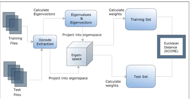
We start with the initial matrix A[M, N], here N is maximum file size among available virus files andM is total number of virus files used for training. This matrix is fed to the Matlab tool that executes the algorithm steps discussed in Section 5.1. It generates eigenspace and computes weights for each virus file. This constitutes to the training set.

Test set is generated by computing weights for each virus file with respect to the eigenspace created in the training set. Finally,we calculate distance between the weight vectors of training set and test set and determine if the test file belongs to the training set.

The process is summarized in Figure 10.

6.4 Setup

Table 1 shows the experiment setup we used to carry out the experiment. Table 1: Experiment setup

Type Description

Operating System Linux Ubuntu 11.2, 32-bit Matlab R2011b

CHAPTER 7 Experimental Results

In our experiment we carried out testing for different virus families as listed in Table 2. For limited number of test files, we used the five fold cross validation method to generate ample number of test sets. We chose 80% of available files for training and the rest are allocated for testing. For the next round of testing, we strategically shuffle the files in the training set and the test set. This gives advantage of producing more data for testing while reducing the data bias.

Table 2: Virus families

Virus Operating System Total Training Files Testing Files

G2 Windows 50 40 10

MPCGEN Windows 50 40 10

NGVCK Windows 50 40 10

MWOR Linux 800 50 750

Table 3 shows various benign files used for testing. The cygwin files are tested along with windows executable virus such as NGVCK. For MWOR, we used linux benign files, the same that are used for dead code insertion in the worm. This provides more challenging test for MWOR files.

Table 3: Benign Files

Benign Files Description Total

Cygwin Files Executables from cygwin utility 33 Linux Files Linux binaries 11

7.1 Results

plot-value of the euclidean distance, denotes that the test file is closer to the training set.

7.1.1 G2

Figure 11 displays graph for G2 virus files. Here, both cygwin and linux files are tested against the training set of G2 virus files. Our technique can detect all G2 virus files and benign files accurately, giving 0% false positive and 0% false negative results.

Figure 11: G2 virus

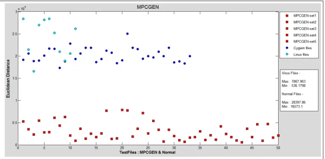
7.1.2 MPCGEN

Similar to the G2 files, we computed a training set, using MPCGEN files. Both cygwin andl linux files are tested along with the virus files. Figure 12 shows a clear

Figure 12: MPCGEN virus

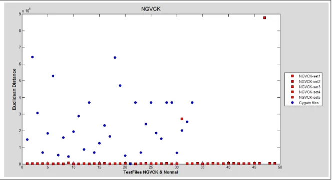
7.1.3 NGVCK

NGVCK is a more complex virus than MPCGEN and G2. It uses multiple morphing techniques to create different virus instances [11]. Our detection technique offers quite good results maintaining the value of false positive and false negative rates to minimum. As shown in Figure 13, out of 50 test files only 2 files are falsely detected as benign and one of the benign files is detected as a virus by the system.

7.1.4 MWOR

MWOR is a metamorphic worm developed as a part of academic research [17]. It uses two metamorphic techniques: equivalent instruction substitution, and dead code insertion. The percentage of dead code inserted can be given by a “padding ratio”, where the padding ratio is the number of dead instructions divided by the number of instructions that constitute core functionality of the worm. For example, MWOR with a padding ratio of 0.5 indicates that 50% as much as the actual virus instructions

Figure 13: NGVCK virus

are inserted in the virus to obfuscate its functionality. We tested approximately 750 files ranging from 50% to 400% of the dead code. The scores for virus and benign linux files are shown in Figure 14. Our technique works well in detecting a high level morphed copy of the MWOR virus.

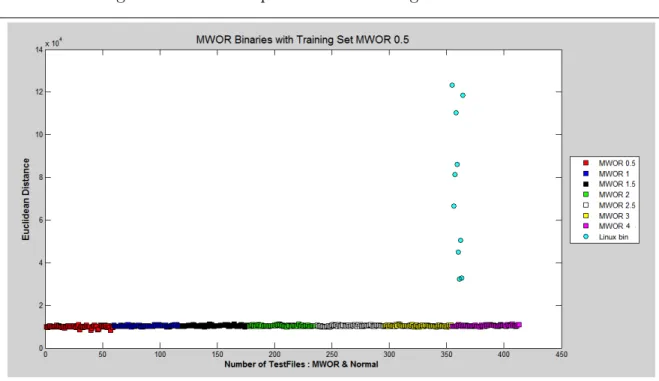
7.2 Results for MWOR binaries

We performed similar tests using binaries instead of opcodes. Opcodes as well as operands are extracted for binaries and processed to create eigenspace. Figure 15 shows the results for testing MWOR files. In this case, we used the training set containing binaries of MWOR with padding ratio 0.5. Based on the graph, it can be seen that MWOR binaries outperformed the opcode technique. We speculate that the lack of operand data in case of opcodes technique causes it to loose accuracy in

Figure 14: MWOR opcodes with training set MWOR 0.5

Figure 15: MWOR binaries with training set MWOR 0.5

7.3 Receiver Operating Characteristic (ROC) Curves

[21]. The true positive rate of the test is plotted against the false positive rate. The accuracy of the test depends on how well the test distinguishes between true positives and false positives among the available data set. When data points are plotted based on the results of the test, the area enclosed inside the graph is called Area under Curve (AUC).

The AUC represents if the test is accurate for a given data set. AU C = 1.0 represents a perfect test as it gives a 100% true positive rate and a 0% false positive rate. Based on the results in section 7.1, we plotted ROC curves for all virus families to analyze effectiveness of our technique.

Table 4 shows the AUC statistics for all virus families along with their standard error rate. The same for MWOR are shown in Table 5. Figure 16, 17, 18, 19 show the ROC curves for MWOR, NGVCK, MPCGEN and G2 virus respectively.

Table 4: AUC Statistics for virus families

Virus AUC Standard Error

G2 1 0

MPCGEN 1 0

NGVCK 0.94727 0.02812

7.4 AUC statistics

For the comparison purpose, we produce the standard error tables for both op-code and binary approach for MWOR virus in Table 5 and 6 respectively. The AUC tables demonstrate that Eigenviruses technique outperformed HMM based detection technique as shown in Table 6 and Table 7.

Figure 16: ROC for MWOR

Table 5: AUC Statistics for MWOR with training set of MWOR 0.5

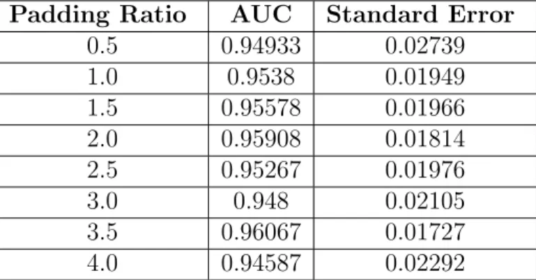
Padding Ratio AUC Standard Error

0.5 0.94933 0.02739 1.0 0.9538 0.01949 1.5 0.95578 0.01966 2.0 0.95908 0.01814 2.5 0.95267 0.01976 3.0 0.948 0.02105 3.5 0.96067 0.01727 4.0 0.94587 0.02292

Figure 17: ROC for NGVCK

Table 6: AUC Statistics for MWOR binaries with training set of MWOR 0.5

Padding Ratio AUC Standard Error

0.5 1 0 1.0 1 0 1.5 1 0 2.0 1 0 2.5 1 0 3.0 1 0

Figure 18: ROC for MPCGEN

Table 7: AUC statistics for MWOR using HMM detection

Padding Ratio AUC Standard Error

0.5 1 0 1.0 0.99 0.0105 1.5 0.9625 0.03503 2.0 0.9725 0.02112 2.5 0.8325 0.06556 3.0 0.8575 0.06225 4.0 0.8225 0.06661

CHAPTER 8 Conclusion

Metamorphic virus detection is a challenging task. There have been many at-tempts to detect highly metamorphic virus in the past [9] [18] [3] [2] [1]. We imple-mented an eigenviruses technique mentioned in the Eigenviruses paper [11]. After successful detection of NGVCK virus files, we proceeded to implement the same technique using a different approach. We used opcodes of virus files instead of raw binaries. It is observed that this approach is more accurate because it focuses on more relevant code information and avoids processing extraneous operand data.

We implemented our proposed approach and analyzed the results by testing various metamorphic virus families such as G2, MPCGEN, NGVCK and MWOR. The technique gave more than 94% accurate detection of virus files. When two approaches are compared, the opcode approach provided a more convergent graph for the virus files from the same family. Better segregation between scores of benign and virus files proved to be crucial in classification. We also employed variations in the test to improve computational efficiency. It is observed that only 20% of total eigenvectors suffice to effectively detect all virus files, keeping false positive and false negative rates low.

Very few virus detection techniques materialize in an antivirus product due to their computational infeasibility and high rate of false positives. Based on the results of this technique, we believe it can aptly complement traditional antivirus products.

8.1 Future work

Due to limited time and resources, only four well-known metamorphic viruses were tested. As part of future testing efforts, the proposed system should be vali-dated with well-known and hard-to-detect metamorphic viruses such as W95/Zmist, W95/Zperm or W95/Bistro.

We used separate training sets for each virus family. It will be interesting to see the results when single training set containing samples of each virus family is used to train the model. Threshold for each virus family can be heuristically set to identify a test le.

With a higher number of virus families the euclidean distance may not provide accurate results. Instead, a more effective Mahalanobis distance can be used. It takes into account the correlation of the data set and also its scale-invariant [10]. It can help us perform cluster analysis of the metamorphic viruses which then can be classified in families.

Code packing is a common technique that transforms executable virus code into data as a post-processing stage in the malware development cycle. At run time, the data, or hidden code, is restored to its original executable form through dynamic code generation using an associated restoration routine. In order to reduce the errors while detecting such virus, some malware normalization techniques can be used to preprocess the virus replicates. A depermutator may help recognize and extract the real virus code. With such preprocessing for the test file, we believe that the system performance can be improved.

LIST OF REFERENCES

[1] Al-Shbail A., Al-Smadi A., Daoud E., Detecting metamorphic viruses by us-ing arbitrary length of control flow graphs and nodes alignment. In ICIT 2009 Conference - Bioinformatics and Image, 2009, 4, (3), pp. 628–633.

[2] Ando R., Nguyen A., Takefuji Y., Resolution based metamorphic computer virus detection using redundancy control strategy. In WSEAS Conference, 2005. [3] Attaluri S., McGhee S., Stamp M., Profile hidden markov models and

metamor-phic virus detection. Journal in Computer Virology, 2011, 5(2).

[4] Babak R., Daud Z., Ibrahim S., Masrom M., Morphing engines classification by code histogram. In Symposium on Information & Computer Sciences, 2011. [5] Daoud E., Jebril I., Computer virus strategies and detection methods.

Interna-tional Journal of Open Problems Computer Mathematics, 2006, 1(2).

[6] Eigenvalues and eigenvectors. http://ceee.rice.edu/Books/LA/eigen/ [Re-trieved on October 2012].

[7] Eigenvector. http://mathworld.wolfram.com/Eigenvector.html [Retrieved on

March 2012].

[8] Evgenios S., Konstantinou M., Metamorphic virus: analysis and detection, February 2008.

[9] Ferrie P., Szor P., Hunting for metamorphic. In Virus Bulletin Conference, September 2001, pp. 123144.

[10] Mahalanobis Distance. http://en.wikipedia.org/wiki/Mahalanobis_distance

[Retrived on December 2012].

[11] Mohamed A., Nabi A., Saleh M., Eigenviruses for metamorphic virus recognition. In IET Information Security, 2011, 5(4), 191-198.

dx.doi.org/10.1049/iet-ifs.2010.0136.

[12] Nachenberg C., Computer virus coevolution. In Communications of the ACM, 1997, 50, (1), pp. 46-51.

[13] PE Header extraction.

[14] Pentland A., Turk M., Eigenfaces for recognition. Journal of Cognitive Neuro-science, 1991, 3, pp. 71-86.

[15] Rabiner L., A tutorial on hidden markov models and selected applications in speech recognition. In Proceedings of the IEEE, 1989, 77, (2), pp. 257–286. [16] Runwal N., Graph technique for metamorphic virus detection.Master’s Projects,

Paper 206, Department of Computer Science, San Jose State University, Decem-ber 2011.

[17] Sridhara S., Stamp M., Metamorphic worm that carries its own morphing engine.

Journal in Computer Virology, October 2012.

[18] Stamp M., Wong W., Hunting for metamorphic engines. Journal in Computer Virology, 2006, 2, (3), pp. 211-219.

[19] Symantec corporation: Internet security threat report. April 2010, vol. XV, p. 21.

[20] Szor P.,The art of computer virus research and defense, Addison-Wesley Profes-sional, 2005.

[21] The area under an ROC curve. http://gim.unmc.edu/dxtests/roc3.htm

[Re-trived on December 2012].

[22] Virus source.http://cs.sjsu.edu/~stamp/viruses/[Retrived on October 2012].

[23] Wong W., Analysis and detection of metamorphic computer viruses. Master’s Projects, Paper 153, Department of Computer Science, San Jose State Univer-sity, 2006. http://www.cs.sjsu.edu/faculty/stamp/students/Report.pdf

APPENDIX A Opcode to Bytecode Map

Byte code Opcode

01 ADD 06 PUSH 07 POP 08 OR 10 ADC 18 SBB 27 DAA 28 SUB 2F DAS 30 XOR 37 AAA 38 CMP 3F AAS 60 PUSHA 60 PUSHAD 61 POPA 61 POPAD 62 BOUND 63 ARPL 69 IMUL 70 JO 6D INS 6D INSB 6E OUTS 6E OUTSB 6F OUTS 6F OUTSW 71 JNO 72 JB 72 JNAE 72 JC 73 JNB 73 JAE 73 JNC

Table A.8 –Continued from previous page Byte code Opcode

74 JE 75 JNZ 75 JNE 76 JBE 76 JNA 77 JNBE 77 JA 78 JS 79 JNS 7A JP 7A JPE 7B JNP 7B JPO 7C JL 7C JNGE 7D JNL 7D JGE 7E JLE 7E JNG 7F JNLE 7F JG 84 TEST 86 XCHG 88 MOV 8D LEA 90 PAUSE 98 CBW 98 CWDE 99 CWD 99 CDQ 9A CALLF 9B FWAIT 9B WAIT 9C PUSHF 9C PUSHFD 9D POPF 9D POPFD

Table A.8 –Continued from previous page Byte code Opcode

A4 MOVS A4 MOVSB A5 MOVSW A5 MOVSD A6 CMPS C8 ENTER C9 LEAVE CA RETF CC INT CE INTO D0 ROL D0 ROR D0 SHL D8 FDIV D9 FLD D9 FNOP E0 LOOPNZ E0 LOOPNE E1 LOOPZ E1 LOOPE E2 LOOP E3 JCXZ E3 JECXZ E4 IN E6 OUT E8 CALL E9 JMP EA JMPF F2 REPNZ F2 REPNE F2 REP F6 DIV F6 IDIV F7 NOT F7 NEG F7 MUL F8 CLC FE DEC FF JMPF

APPENDIX B Additional Graphs B.1 Euclidean distance Graphs

B.1.1 MWOR with consolidated training set

Graph B.20 displays the scores for MWOR files when tested against the training set containing consolidated training set.

Figure B.20: MWOR virus with consolidated training set

B.1.2 MWOR with different training sets

Graph B.21 displays the scores for MWOR files when tested against different training sets.

Figure B.21: MWOR virus with consolidated training set

B.1.3 MWOR with 20% eigenvectors

Graph B.22 displays the scores for MWOR files when tested against the eigenspace constructed by 20% of total eigenvectors.

B.1.4 MWOR with 6% eigenvectors

Figure B.23 shows the results when only 6% of total eigenvectors are considered to construct a training set.

B.1.5 NGVCK with 20% eigenvectors

Figure B.24 shows the results for NGVCK. We can see that scores for benign files are closer to virus files when only 20% of eigenvectors are used.

Figure B.22: MWOR virus with 20% eigenvectors

Figure B.23: MWOR virus with 6% eigenvectors

B.1.6 NGVCK with 6% eigenvectors

Figure B.24: NGVCK virus with 20% eigenvectors files such that they become indistinguishable.

B.2 ROC Graphs

B.2.1 ROC for MWOR with 20% eigenvectors

Graph B.26 shows ROC for MWOR files when 20% of total eigenvectors are used.

Figure B.26: ROC : MWOR with 20% eigenvectors

B.2.2 ROC for MWOR with 6% eigenvectors

Graph B.27 shows ROC for MWOR files when 6% of total eigenvectors are used.

Figure B.27: ROC : MWOR with 6% eigenvectors

B.2.3 ROC for MWOR Binary files

Text section from MWOR binaries are extracted and used to create eigenvectors. Method offers good classification among MWOR and benign binaries as shown in Figure B.28.

B.2.4 ROC for NGVCK with 20% eigenvectors

Figure B.28: ROC : MWOR binaries

B.2.5 ROC for NGVCK with 6% eigenvectors

Graph B.30 shows ROC for NGVCK files when 6% of total eigenvectors are used.

AU C = 0.942

B.2.6 ROC for NGVCK binary files