Inflation forecasting in the new EU Member States

by Olga Arratibel,

Christophe Kamps

and Nadine Leiner-Killinger

InflatIon

forecastIng In

the new eU

MeMber states

workIng PaPer serIes

no 1015 / febrUary 2009

W O R K I N G PA P E R S E R I E S

N O 1015 / F E B R U A R Y 2 0 0 9

This paper can be downloaded without charge from http://www.ecb.europa.eu or from the Social Science Research Network electronic library at http://ssrn.com/abstract_id=1334129. In 2009 all ECB

publications feature a motif taken from the €200 banknote.

INFLATION FORECASTING IN THE

NEW EU MEMBER STATES

by Olga Arratibel

_,

Christophe Kamps

and Nadine Leiner-Killinger

1 We would like to thank, without implying, Hans-Joachim Klöckers, Ricardo Mestre, Philippe Moutot, Ad van Riet, Philipp Rother, Jean-Pierre Vidal and participants at the European Commission Workshop “What drives inflation in the new EU Member States?” for their valuable comments and suggestions. We also thank an anonymous referee for helpful comments. The views expressed are our own and do not necessarily

© European Central Bank, 2009 Address

Kaiserstrasse 29

60311 Frankfurt am Main, Germany

Postal address

Postfach 16 03 19

60066 Frankfurt am Main, Germany

Telephone +49 69 1344 0 Website http://www.ecb.europa.eu Fax +49 69 1344 6000

All rights reserved.

Any reproduction, publication and reprint in the form of a different publication, whether printed or produced electronically, in whole or in part, is permitted only with the explicit written authorisation of the ECB or the author(s).

The views expressed in this paper do not necessarily refl ect those of the European Central Bank.

The statement of purpose for the ECB Working Paper Series is available from the ECB website, http://www.ecb.europa. eu/pub/scientific/wps/date/html/index. en.html

Abstract 4

Non-technical summary 5

1 Introduction 6

2 Infl ation developments and infl ation

forecasts in the NMS: stylised facts 7

2.1 Non-monetary determinants of infl ation

in the new EU Member States 10

2.2 Monetary determinants of infl ation

in the new EU Member States 13

3 The empirical framework 14

3.1 Data 14

3.2 Methodology 16

4 Empirical results 20

4.1 Short-term forecast of infl ation

developments (4 quarters ahead) 21

4.2 Long-term forecast of infl ation

developments (12 quarters ahead) 24

5 Conclusions 28

References 29

Appendix 31

European Central Bank Working Paper Series 37

Abstract

To the best of our knowledge, our paper is the first systematic study of the predictive power of monetary aggregates for future inflation for the cross section of New EU Member States. This paper provides stylized facts on monetary versus non-monetary (economic and fiscal) determinants of inflation in these countries as well as formal econometric evidence on the forecast performance of a large set of monetary and non-monetary indicators. The forecast evaluation results suggest that, as has been found for other countries before, it is difficult to find models that significantly outperform a simple benchmark, especially at short forecast horizons. Nevertheless, monetary indicators are found to contain useful information for predicting inflation at longer (3-year) horizons.

Keywords: Inflation forecasting, leading indicators, monetary policy, information content of money, fiscal policy, New EU Member States

Non-technical summary

In recent years inflation has accelerated, sometimes very sharply, in most of the non-euro area EU Member States that have joined the EU since 2004 (hereafter, the new EU Member States: NMS). The recent rise in inflation has been largely attributed to a series of adverse supply shocks, such as energy and food price increases, as well as to ongoing changes in the economic structures of these catching-up economies. At least in some countries, capacity pressures also seem to have played a role. Accordingly, the rise in inflation would appear by and large inevitable and, as regards the occurrence of adverse shocks, unpredictable. Indeed, over the past few years, inflation forecasts by international organisations and other professional forecasters appear to have sharply underestimated the recent rise in inflation in the NMS. The question arises whether the recent rise in inflation could have been predicted better by accounting for the signals of monetary indicators like trend money growth, which have not received much attention in discussions of recent inflation developments in the NMS. Against this background, this paper (1) analyses potential economic and fiscal variables as explanatory variables for inflation developments and (2) takes a close look at the leading indicator properties of monetary and credit aggregates for future inflation. It focuses on inflation developments in eight Central and East European EU Member States, namely Bulgaria, the Czech Republic, Estonia, Latvia, Lithuania, Hungary, Poland and Romania. To the best of our knowledge, this paper is the first systematic study to analyse the performance of a large set of monetary, economic and fiscal indicators in explaining inflation dynamics in the NMS, including bivariate models and trivariate (two-pillar Phillips curve) models. Three findings can be highlighted. First, we find that the performance of alternative forecasting models differs substantially across countries in that different variables seem to be influencing to a different extent inflation developments at different forecast horizons. Second, at the short-term (one-year) horizon, with the exception of a few countries, it is difficult to find models with forecasts significantly outperforming those of a simple benchmark (the random walk model). This finding is in line with empirical results for the U.S. and other OECD countries suggesting that inflation has become increasingly hard to forecast. In the few countries for which we find forecasting models significantly outperforming the benchmark at the one-year horizon, such models are in general based on economic and fiscal indicators. Third, we find that, over the longer term (three-year) forecasting horizon, monetary indicators contain useful information for predicting inflation in most NMS countries. Interestingly, the role played by monetary factors in driving inflation dynamics does not differ substantially between the NMS with a fixed exchange rate regime and those with a floating exchange rate regime. Thus, monetary indicators appear to become important variables to explain inflation trends across the majority of the NMS over the long-term forecasting horizon.

“Inflation is always and everywhere a monetary phenomenon”

(Milton Friedman (1963), Inflation: Causes and Consequences, Asia Publishing House, New York.)

1. Introduction

In recent years inflation has accelerated, sometimes very sharply, in most of the non-euro area EU Member States that have joined the EU since 2004 (hereafter, the new EU Member States: NMS). The recent rise in inflation has been largely attributed to a series of adverse supply shocks, such as energy and food price increases, as well as to ongoing changes in the economic structures of these catching-up economies. At least in some countries, capacity pressures also seem to have played a role. Accordingly, the rise in inflation would appear by and large inevitable and, as regards the occurrence of adverse shocks, unpredictable. Indeed, over the past few years, inflation forecasts by international organisations and other professional forecasters appear to have sharply underestimated the recent rise in inflation in the NMS. The question arises whether the recent rise in inflation could have been predicted better by accounting for the signals of monetary indicators like trend money growth, which have not yet received much attention in discussions of recent inflation developments in the NMS. The extent of monetary accommodation could be expected to be a key determinant of the transmission of shocks to inflation over medium-term to long-term horizons.

Against this background, this paper attempts to answer the following questions: To what extent do the above mentioned non-monetary factors explain the rise in inflation in these countries? Why has the rise in inflation over recent years been so heterogeneous across the NMS in the presence of common external shocks and similar levels of economic development? What is the role of money in explaining inflationary developments in the NMS? Could the rise in inflation, and also its heterogeneity across NMS, have been predicted? To address these questions this paper (1) analyses potential economic and fiscal variables as explanatory variables for inflation developments and (2) takes a close look at the leading indicator properties of monetary and credit aggregates for future inflation. It focuses on inflation developments in eight Central and East European EU Member States, namely Bulgaria, the Czech Republic, Estonia, Latvia, Lithuania, Hungary, Poland and Romania. Depending on data availability, the time period analysed in this paper is 1993Q1 to 2008Q2. To the best of our knowledge, our paper is the first systematic study of the predictive power of monetary aggregates for future inflation in the eight NMS. Individual-country studies exist for a few NMS, see e.g. Dabusinskas (2005) and Kotlowski (2005). These studies in general conclude that monetary aggregates provide useful information for forecasting inflation. Our forecast evaluation exercise builds on the empirical framework first applied by Stock and Watson (1999) to U.S. data and subsequently applied by Nicoletti-Altimari (2001),

Carstensen (2007) and Hofmann (2008) to euro area data.1 In this exercise, we consider a large set of monetary and non-monetary (economic and fiscal) indicators.

We find that the performance of alternative forecasting models differs substantially across countries in that different variables seem to be influencing to a different extent inflation developments at different forecast horizons. We also find that at the 4-quarter horizon, with the exception of a few countries, it is difficult to find models with forecasts significantly outperforming those of a simple benchmark (the random walk model). This result is in line with the findings of Stock and Watson’s (2008) literature review suggesting that inflation has become increasingly hard to forecast in the U.S. and other OECD economies. However, our results also suggest that, over the longer term (3-year) forecasting horizon, monetary indicators contain useful information for predicting inflation in most NMS countries.

The paper is organised as follows. Section 2 first reviews past inflation developments and assesses inflation forecasts for the eight NMS. It then provides stylised facts on monetary and non-monetary (economic and fiscal) factors that have contributed to inflation developments in the NMS. Section 3 discusses the data and methodology used in the forecast evaluation exercise and Section 4 presents the empirical results. Section 5 concludes, highlighting the implications of monetary indicators for future inflation developments in the NMS.

2. Inflation developments and inflation forecasts in the NMS: stylised facts

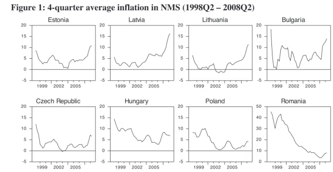
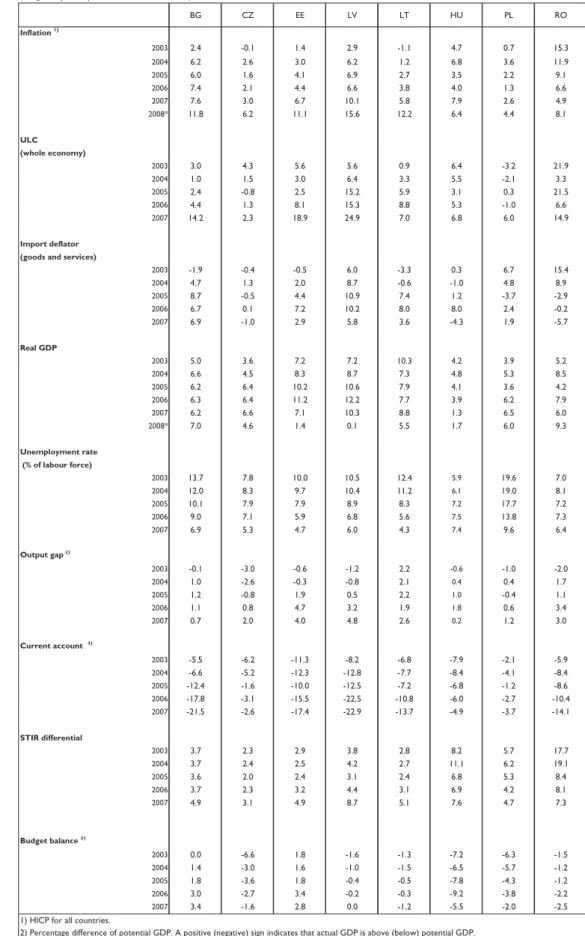
Since the end of the 1990s until the beginning of this decade inflation rates in most NMS followed a broadly downward path from relatively high levels (see Figure 1). At different points in time between 2003 and 2005, this pattern started to change quite noticeably. First, the disinflation process was interrupted in all countries but Romania. Second, inflation started to increase again, in some countries to remarkably high levels. Third, while the process of disinflation until around 2003 had taken place irrespective of the exchange rate strategy chosen, the rise in inflation over the period 2004-08 has been particularly virulent in the countries that have opted for “hard-pegs” (i.e. the Baltic States and Bulgaria). In the other countries, which follow an inflation-targeting strategy allowing for a higher degree of exchange rate flexibility (hereafter, “the floaters”), the surge in inflation has been generally more contained. Although the economic cycle seems to have peaked in 2008 in many cases, most notably in the Baltic States, strong price pressures remain (see for a survey of economic indicators for the NMS Table A.1 in the Appendix).

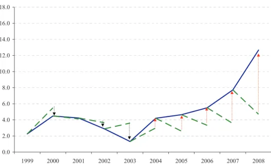
In such a changing environment, trying to predict the behaviour of price dynamics has become particularly demanding. This is illustrated in Figure 2 below, which shows for the

1 _{For other methodologies to forecast inflation in the euro area see e.g. De Santis et al. (2008), Hubrich (2005),} Calza et al. (2001). These models tend to require relatively large numbers of observations and a stable

eight countries considered and for the years 1999-2008, the annual average inflation rate and the respective inflation forecast that was made 18-months ahead, prior to the release of the final outcome. For example, the forecast for the average annual inflation in 2004 is the one

made in May-June 2003. The forecasts have been taken from the Eastern Europe Consensus

Forecast.

Figure 1: 4-quarter average inflation in NMS (1998Q2 – 2008Q2)

Estonia 1999 2002 2005 -5 0 5 10 15 20 Czech Republic 1999 2002 2005 -5 0 5 10 15 20 Latvia 1999 2002 2005 -5 0 5 10 15 20 Hungary 1999 2002 2005 -5 0 5 10 15 20 Lithuania 1999 2002 2005 -5 0 5 10 15 20 Poland 1999 2002 2005 -5 0 5 10 15 20 Bulgaria 1999 2002 2005 -5 0 5 10 15 20 Romania 1999 2002 2005 0 10 20 30 40 50

Note: 4-quarter average inflation is defined as 100*ln(CPIt/CPIt-4).

Interestingly, until 2003 inflation outcomes surprised on average on the downside: with the main exception of the floaters in the year 2000, inflation turned out rather close to and, at times, below the inflation forecast expected by the Consensus Forecast 18 months before. Thereafter, however, inflation has surprised on the upside, particularly in the last two years. Moreover, developments across countries have started to diverge. Specifically, forecasting inflation dynamics in the “hard-peg” countries seems to have become a particularly challenging task, with the forecasts having underpredicted inflation five years in a row. The question arises whether this systematic underprediction of future inflation was unavoidable given a series of unpredictable unfavourable shocks or whether the forecasts missed important information that would have allowed avoiding a downward bias.

Figure 2 Inflation forecasts and actual inflation (1999-2008)

"HARD-PEGS" - Inflation and 18-months ahead inflation forecasts* (annual average, CPI index, %)

0.0 2.0 4.0 6.0 8.0 10.0 12.0 14.0 16.0 18.0 1999 2000 2001 2002 2003 2004 2005 2006 2007 2008

Source: Eastern Europe Consensus Forecasts and IMF (International Financial Statistics).

* Unweighted average of annual inflation rates in Bulgaria, Estonia, Latvia and Lithuania. The arrows heading up (down) denote higher (lower) than expected inflation.The value for 2008 indicates the latest data available (August 2008).

"FLOATERS" - Inflation and 18-months ahead inflation forecasts* (annual average, CPI index, %)

0.0 2.0 4.0 6.0 8.0 10.0 12.0 14.0 16.0 18.0 1999 2000 2001 2002 2003 2004 2005 2006 2007 2008

Source: Eastern Europe Consensus Forecast and IMF (International Financial Statistics) .

* Unweighted average of annual inflation rates in the Czech Republic, Hungary, Poland and Romania. The arrows heading up (down) denote higher (lower) than expected inflation. The value for 2008 indicates the latest data available (August 2008).

The forecast evaluation exercise presented in Sections 3 and 4 attempts to shed light on this question. In this exercise the “naïve” random walk model will serve as the benchmark to evaluate the performance of alternative forecasting models. As has been shown in the forecasting literature, it has proven difficult to find model-based forecasts or forecasts by professional forecasters that significantly outperform this simple benchmark (see, e.g., Stock and Watson 2007). Visual inspection of Figure 2 confirms that for our set of countries the Consensus forecasts in general did not outperform the simple no-change forecast implied by the random walk model. Going beyond visual impression, we computed a simple metric of forecast performance, the root mean squared forecast error, over the period 2003-08 both for the Consensus forecasts and for the random walk model (in the latter case using the average annual inflation rate over the previous twelve months in June of a given year as the forecast for average annual inflation in the next year). These computations confirm that across our set of countries on average the random walk model performed equally well than the Consensus forecasts, with the latter performing slightly better than the random walk model in the

“floating” countries but worse in the “hard-peg” countries.2 Given these findings and also

because only too narrow a set of Consensus forecasts is available, we use the random-walk model as the benchmark in our formal forecast evaluation exercise presented below.

Before turning to this exercise, several non-monetary economic and fiscal as well as monetary factors are analysed with respect to their potential impact on inflation developments in the NMS.

2.1 Non-monetary determinants of inflation in the new EU Member States

The rise in inflation in the NMS has generally taken place against the background of dynamic economic conditions, with external factors also having played a role. On the domestic side, strong domestic demand, underpinned by robust growth in disposable income, large inflows of foreign direct investment, low real interest rates and buoyant credit growth, have

contributed to inflationary pressures in most NMS.3 Moreover, the rapid tightening of the

labour market, exacerbated by labour outflows to other EU countries, has contributed to rapid increases in wages, often significantly above labour productivity growth, hence leading to high growth in unit labour cost, particularly in the fastest growing economies. Under such circumstances, capacity constraints and signs of overheating emerged in many countries, e.g

the Baltic States, Bulgaria, the Czech Republic and Romania.4

2 _{Romania is a clear outlier, for which the random-walk model performs very poorly because it misses the strong} downward trend in inflation over the sample period, which at least to some extent was predictable.

3 _{The main exception would be Hungary, where output growth has remained relatively subdued.}

4 _{In most NMS, notably in those that have opted for a “hard-peg” to the euro, the process of catching-up in real} income with the euro area is likely to manifest itself in higher inflation. However, the exact size of such effect is difficult to assess. According to most studies, it generally accounts for between 0.4 and 2.4 percentage points of inflation in the NMS (see Darvas and Szapáry (2008)).

As for the external factors, among the most important drivers of inflation in the NMS are food prices, which had been declining in 2001-03 but have since rebound sharply, and soaring energy prices. These two components have a relatively large weight in the consumption basket of these countries, representing around 43% of the total (61.2% in the case of Romania). In some countries with flexible exchange rates, these price increases have been partly dampened by an appreciating currency (i.e. the Czech Republic and Romania). Moreover, the impact of globalisation and strong competition, noticeably from emerging Asia, seem to have generally contributed to containing growth rates in the price of tradable goods (e.g. textiles, furniture, IT equipment) in many NMS.

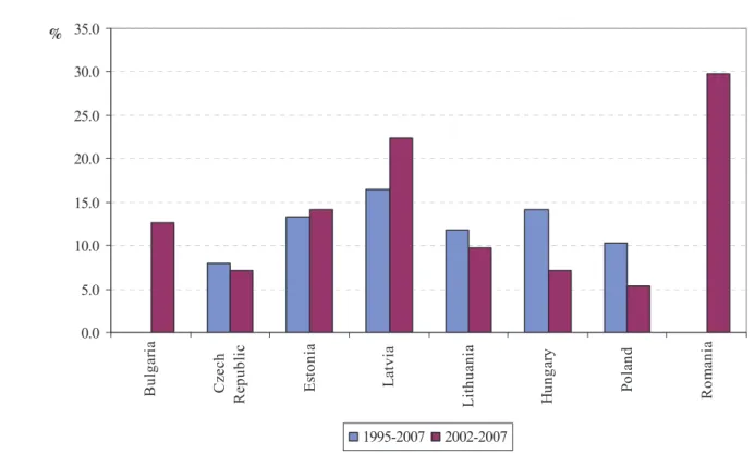
Also fiscal policy, through the impact of, inter alia, public finance reform, the fiscal stance, changes in direct and indirect taxation, public wage-setting as well as the liberalisation of administered prices in the wake of EU entry affected inflation performance in the NMS. In several of the eight NMS considered here, direct taxes and social security contributions were lowered in an attempt to reduce tax wedges and thus increase labour supply in the presence of labour shortages and sometimes large shadow economies in these fast growing economies. To the extent that capacity constraints were lowered, these measures contributed to containing inflation. At the same time, to the extent that these measures raised domestic demand, they tended to contribute to a rise in inflation. Furthermore, in several NMS, public wages rose significantly. As Figure 3 indicates, the increase in government spending on compensation of public employees in the general government sector reached double digit values in the Baltic countries, Hungary and Poland between 1995 and 2007. In Bulgaria and the Baltic countries, which faced a strong pick-up in inflation since 2003, compensation of public employees over this period continued to rise at these high rates. At the same, apart from Romania, it fell in those NMS with disinflation, such as in Hungary and Poland, or continued to grow at relatively lower growth rates, such as in the Czech Republic.

Figure 3: Compensation of public employees, general government (annual average percentage changes) 0.0 5.0 10.0 15.0 20.0 25.0 30.0 35.0 Bulga ria Czech R epub li c Es to ni a L atvia L it hua nia H ung ar y Po la nd Ro m an ia % 1995-2007 2002-2007

Notes: For Romania 2003-2007, for Hungary 1997-2006. Source: ESCB, ECB calculations.

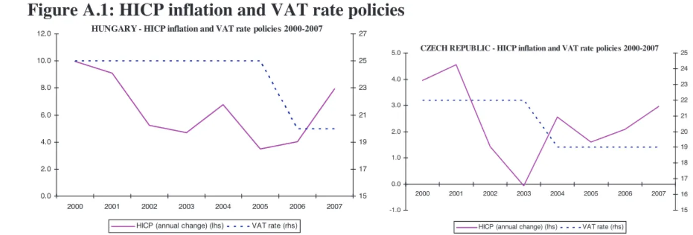
Furthermore, the liberalisation of administered prices in sectors such as e.g. energy and transport contributed to price increases that varied across the NMS. As regards indirect taxes, over the last decade, three of the eight NMS considered lowered their VAT rates, partly substantially in view of EU tax harmonisation, namely the Czech Republic, Hungary and

Romania.5 While in Romania these measures took place in a disinflation environment, they

were followed by a pick-up in inflation in the others. Moreover, most of the NMS receive partly substantial EU Structural Funds within the EU cohesion policy framework that may affect inflation. In 2007, the allocation of EU Funds to the eight NMS considered here amounted to about 2½% of GDP on average. While these funds are aimed at improving long-term growth and employment prospects in the supported regions they may in the short run raise domestic demand significantly, thus raising inflation particularly at times of capacity

constraints.6 As regards fiscal policy, overall, fiscal efforts to comply with the requirements of

the Stability and Growth Pact tended to foster fiscal consolidation in the NMS that should in

5 _{In Hungary, the VAT rate was lowered by 5 percentage points to 20% in 2006, and in the Czech Republic by 3} percentage points to 19% in 2003 (see Figure A.1 in the Appendix). In Romania the VAT rate was reduced by 3 percentage points to 19% in 2000.

6 _{See for details Kamps et al. (2009). It is, however, difficult to gauge the impact of these funds on inflation as} one has to disentangle allocations from actual payments, which do not coincide in general. Due to data limitations, we cannot account for the role of EU funds in our forecasting exercise.

principle have worked in the direction of inflation containment. Nevertheless, one may conjecture that, at times, a loosening fiscal stance, resulting from e.g. high capital spending in the presence of large infrastructure needs and measures to raise labour supply, may have contributed to an increase in inflation. In addition, at some instances, the fiscal stance has not been tight enough to sufficiently contribute to inflation containment (see Figure A.2 in the Appendix).

2.2. Monetary determinants of inflation in the new EU Member States

The economic and fiscal determinants of inflation developments in the NMS share the

following feature: it is often unanticipated shocks to these variables and their more or less

sluggish propagation what drives inflation developments over the short to medium run.

Shocks to food and energy prices, for example, not only heavily affect relative prices but, in the short to medium run, also strongly affect overall inflation. However, in the long run such shocks need not impact on overall inflation unless monetary policy chooses to at least partly accommodate them. This subsection presents one indicator of monetary-policy induced inflationary pressures, namely the evolution of trend money growth.

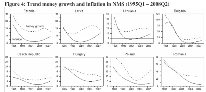
The empirical literature has established a strong link between money growth and inflation for OECD countries, looking at data that span more than a century (see, e.g., Lucas 1996 and Benati 2008). This evidence suggests that surges in money growth in general precede high-inflation episodes, making money growth a potentially useful indicator for future high-inflation. More recently, Assenmacher-Wesche and Gerlach (2007, 2008) showed that the empirical link between money growth and inflation is particularly strong at low frequencies, while the relationship is rather noisy at business cycle frequencies. Figure 4 shows the low-frequency components of annualised quarter-on-quarter money growth and inflation for the eight NMS under review for the period 1995 to 2008, where the low-frequency components of the two series have been estimated with a Hodrick-Prescott filter.

The figure reveals a number of interesting findings. First, there has been pronounced disinflation in all eight countries in the second half of the 1990s, accompanied by a strong deceleration in trend money growth. Second, trend inflation and trend money growth started to accelerate in all countries except for Hungary and Romania around the start of the current century. Third, in all these countries the turning point for trend money growth preceded the turning point for trend inflation. On average, trend money growth reached its low point five quarters before trend inflation (median: four quarters) did, with the lead being longest in the case of Latvia (almost three years) and shortest in the case of the Czech Republic (half a year). Also, the pick-up in trend money growth suggests that the recent surge in inflation in the NMS is not exclusively due to the occurrence of unanticipated shocks but at least partly

has monetary roots.7 Fourth, in some countries (Estonia, Latvia and Lithuania) trend money growth peaked in 2005 and decelerated thereafter, suggesting gradually declining inflationary pressures in these countries. All in all, the stylised evidence presented in this subsection suggests that trend money growth contains useful information for predicting future inflation, a hypothesis that will be tested in the remainder of this paper.

Figure 4: Trend money growth and inflation in NMS (1995Q1 – 2008Q2)

Note: Money growth based on broadest available monetary aggregate (M3 for Bulgaria, Hungary and Lithuania, M2 for remaining countries). Trend estimated with Hodrick-Prescott filter (tuning parameter set equal to 1600).

3. The empirical framework

This section presents the empirical framework used to evaluate the performance of alternative forecasting models. The first subsection discusses the data, while the second subsection presents the alternative forecasting models used for this exercise. The empirical results are presented in Section 4.

3.1 Data

We use data for eight NMS, namely Bulgaria, the Czech Republic, Estonia, Latvia, Lithuania, Hungary, Poland and Romania. Most series were retrieved from the Haver Analytics DLX databases “Eurostat”, “EMERGECW” and “IFS” (see Appendix A.2 for details). Most time series are seasonally adjusted by the source. Whenever this is not the case, we seasonally adjust the respective series using the Census X11 multiplicative procedure. Depending on data availability, we use quarterly data for 1993Q1 to 2008Q2. However, data availability differs substantially across countries and for some countries some series start only in the

7 _{Note that even the recent surge in commodity prices (one of the “shocks”) might have been partly driven by} loose monetary policy, albeit at the global level (Frankel 2006).

1990s. For the forecasting regressions, we only used data that were available at least from 1995Q1 onwards. For Bulgaria and Romania, data availability is particularly limited and also data quality appears to be an issue, suggesting that the results for these countries should be taken with a grain of salt.

We group the explanatory variables that we consider in the forecasting exercise into three groups, namely monetary, economic and fiscal indicators. The monetary indicators tested include the monetary aggregates M1, M2 and M3 as well as loan growth. For those countries for which M3 is not available we use M0, M1 and M2 instead. The monetary indicator variables also include concepts such as trend broad money growth, the real money gap, the monetary overhang and the change in P-star (see Appendix A.1 for details).

Economic indicators include both domestic and external factors. Domestic factors comprise the output gap, real GDP growth, employment growth, a measure of the employment gap, the change in the unemployment rate, a measure of the unemployment rate gap, growth in compensation per employee, wage growth, industrial production growth and, finally, the level and change in producers’ selling price expectations as well as consumers’ price expectations based on surveys compiled by the European Commission. External factors include the nominal effective exchange rate, commodity price inflation as well as changes in oil prices. Commodity prices and oil prices expressed in euro are taken from the ECB Monthly Bulletin database and converted into national currency using spot exchange rates.

Fiscal variables comprise growth in general government revenue and expenditure, changes in direct and indirect taxes, changes in VAT revenues, changes in government consumption and growth in compensation of government employees. Unfortunately, a long enough time series of the latter variable is available for the Czech Republic only. However, given that compensation of government employees is by far the largest sub-item in government consumption, one can interpret changes in government consumption as a proxy for government-induced wage pressures.

The trend and gap measures referred to above (e.g. trend money growth and the output gap) are constructed as follows. First, the trend component of the respective variable is estimated with a Hodrick-Prescott filter (with tuning parameter set equal to 1600). We follow Stock and Watson (1999) and Hofmann (2008), using a one-sided filter to estimate the trend components. This filter for each period uses only information up to that period, which is important for the pseudo real-time out-of-sample forecasting exercise we carry out. We estimate the one-sided Hodrick-Prescott filter using the Kalman filter. Once the trend component has been estimated, the gap measure is obtained as the (log) difference between the raw series and the Hodrick-Prescott trend.

3.2 Methodology

The forecast evaluation exercise builds on the empirical framework first applied by Stock and Watson (1999) to U.S. data and subsequently applied by Nicoletti-Altimari (2001),

Carstensen (2007) and Hofmann (2008) to euro area data.8 To the best of our knowledge, our

study is the first attempt to apply this methodology to study the performance of alternative forecasting models for the NMS. The following description of the methodology closely follows Hofmann (2008).

As is common in this literature, we concentrate on single-equation forecasting models with few independent variables for the following reasons. First, single-equation inflation-forecasting models have been found in the forecast evaluation literature to outperform large multiple-equation models such as vector autoregressions or traditional structural macroeconometric models (see, e.g., Stock and Watson 2008). Second, we concentrate on models with few independent variables in order to account for our short data samples. Increasing the number of indicator variables included in the models would quickly exhaust the degrees of freedom. Yet, in order to reflect the large set of information available to professional forecasters in practice, we also present results for combined forecasts that average over the large set of forecasting models (between 40 and 60 per country) we consider in the exercise.

To begin with, the variable to be forecasted has to be chosen. It has become common practice

in the literature to focus on annualised average inflation over the coming h quarters, which

can be formally expressed as h (400/ )ln( _{t h}/ _t)

h

t h CPI CPI

S and where ʌ denotes the

inflation rate and CPI denotes the consumer price index. In the empirical exercise we consider

three alternative forecasting horizons, namely 4-quarter ahead forecasts, 8-quarter ahead

forecasts and 12-quarter ahead forecasts (h = 4, 8, 12).

Benchmark model for forecast evaluation

In order to evaluate the forecasting performance of alternative models, we compare their forecast errors with those obtained for a simple benchmark model. Two candidate benchmark models have been routinely used in the forecasting model. First, the “naïve” random walk

model (hereafter RW), which states that the forecast of h-quarter ahead inflation at time t is

simply the last observable value of h-quarter inflation:

(1) h t h t h t | 1 ˆ S S ,

where )h₁ (400/ )ln( _t1/ _th1

t h CPI CPI

S . Here, we assume as is the case in practice that

the inflation rate at time t, Sth, is not part of the time-t information set.

Second, a univariate autoregressive model for inflation (hereafter AR), which can be expressed as: (2) h h t t h h t E E L S u S _{0 1}( ) ,

where E₁(L) is a finite polynomial of order p in the lag operator L ( p

pL

L

L _{11 1}

1( ) E ... E

E ).

Again, we assume that the inflation rate at time t, St, is not part of the time-t information set.

We follow Carstensen (2007) and use a stepwise procedure to determine which lagged values

of inflation enter the model, considering up to four lagged values of inflation (p 4).9 The h

-quarter ahead forecast, after model estimation, is calculated as t

h t h

t E E L S Sˆ _| ˆ₀ ˆ₁( ) .

The results presented in Section 4 suggest that, in the cross-section of countries considered in this paper and across forecasting horizons, the random walk model on average outperforms the autoregressive model, in the sense that it produces lower root mean squared errors (RMSE). Therefore, we pick the random walk model as the benchmark model when testing whether the alternative forecasting models presented below significantly outperform the benchmark. For this purpose, we use the test for equal predictive ability developed by Diebold

and Mariano (1995), which is applicable in the case of non-nested models.10

Bivariate forecasting models

The first set of forecasting models used in the forecasting exercise extends the univariate

autoregressive model discussed above by including one indicator variable, xt, at a time:

(3) h h t t t h h t E0E1(L)S E2(L)x u S ,

where E₂(L) is a polynomial of order p in the lag operator L. Again, we assume that the

respective indicator variable at time t, xt, is not part of the time-t information set. A stepwise

procedure is used to determine which lagged values of inflation and of the respective indicator variable enter the model, considering up to four lagged values of both inflation and the

9 _{Lagged values enter the model only if they are significant at a pre-specified significance level (here the overall} significance level is set to 0.2). Compared to lag-length selection criteria the stepwise procedure has the advantage of additional flexibility. For example, it might be that lags 1 and 4 turn out to be highly significant but lags 2 and 3 are insignificant. A conventional selection criterion would probably pick a model with one lag only as the best model. However, this would miss the information contained in the fourth lag, which may strongly affect forecast accuracy. The stepwise procedure, instead, would include lags 1 and 4 in the model.

10 _{Note that some of the models are nested, implying non-standard asymptotic distributions under the null}

hypothesis, see Clark and McCracken (2005). Since forecasts are multiple-step, the proper size of the tests would need to be derived by Montecarlo simulation. As doing this for all the models considered in this paper would be

respective indicator variable (p 4). The h-quarter ahead forecast, after model estimation, is calculated as h _tt t h t ˆ ˆ (L) ˆ (L)x ˆ _| E₀ E₁ S E₂ S .

In the empirical exercise the bivariate models are estimated for each country and each indicator variable in turn. The maximum number of bivariate forecasting models is 32 per country, given that we have up to 8 monetary indicators, up to 17 economic indicators and up

to 7 fiscal indicators.11

Trivariate (two-pillar Phillips curve) forecasting models

Gerlach (2003, 2004) proposed a simple trivariate (two-pillar Phillips curve) forecasting model intended to capture at the same time the information of both monetary and economic

indicators. Such trivariate (two-pillar Phillips curve) forecasting models specify h-quarter

ahead average inflation as a function of its own lags, lags of trend broad money growth

( T

t

m

' ), estimated with the one-sided Hodrick-Prescott filter discussed above, as well as lags

of a non-monetary indicator variable (x_t):

(4) h h t T t t t h h t E0 E1(L)S E2(L)x E3(L)'m u S ,

where )E₃(L is a polynomial of order p in the lag operator L. Again, we assume that trend

broad money growth at time t, T

t

m

' , as well as the respective indicator variable at time t, xt,

are not part of the time-t information set. A stepwise procedure is used to determine which

lagged values of inflation, of trend money growth and of the respective indicator variable enter the model, considering up to four lagged values of both inflation and the respective

indicator variable (p 4). The h-quarter ahead forecast, after model estimation, is calculated

as T t t h t h t ˆ ˆ (L) ˆ (L)x ˆ (L)'m ˆ _| E₀ E₁ S E₂ E₃ S .

In the empirical exercise the trivariate (two-pillar Phillips curve) models are estimated for each country and each indicator variable in turn. The maximum number of trivariate (two-pillar Phillips curve) forecasting models is 24 per country, given that we have up to 17

economic indicators and up to 7 fiscal indicators.12

11 _{Given that not all series are available for each country, the effective number of bivariate forecasting models} ranges between 20 (Romania) and 31 (Czech Republic, Estonia, Latvia).

12 _{Given that not all series are available for each country, the effective number of trivariate forecasting models} ranges between 14 (Romania) and 24 (Czech Republic).

Forecast combinations

In addition to the individual-indicator bivariate and trivariate (two-pillar Phillips curve) forecasting models we also provide evidence on the performance of simple forecast combinations. We consider five alternative forecast combinations: combining the forecasts of (i) the monetary-indicator bivariate models, (ii) the economic-indicator bivariate models, (iii) the fiscal-indicator bivariate models, (iv) all bivariate models, and (v) all trivariate (two-pillar Phillips curve) models. All these forecast combinations are computed as the simple average of the forecasts produced by the models with the individual indicators, for each point in time, forecasting horizon and country.

The reason for including these forecast combinations is that such combinations have been shown to significantly improve forecast accuracy in previous studies (see, e.g., Stock and Watson 1999 and Hofmann 2008). Also, forecast combinations based on simple averages have been shown to perform equally well or even better than combinations assigning different weights to the forecasts produced by different models according to some optimality criterion. This result suggests that forecast combinations based on simple averages can best deal with uncertain structural breaks that may heavily affect the forecast performance of individual models. In this context, it may be wise not to assign too much weight to a particular model. These considerations are particularly relevant for our set of countries, characterised by an ongoing convergence process and substantial structural change.

Forecast evaluation sample

In the simulated out-of-sample forecasting exercise, the individual forecasting models are estimated using data prior to the forecasting period in such a way as to reflect the information set available to forecasters in real time. Note, however, that since we lack a real-time database we have to rely on revised data from the most recent vintage of official statistics. In this sense, we conduct a pseudo real-time exercise.

The sample period for the recursive forecasting regressions starts in 1998Q2 for all models, in order to allow for the long lags in the dependent and independent variables. Take the bivariate

model with h=12 as an example. The observation of h-quarter inflation for 1998Q2 (which is

price level in 1998Q2 divided by price level in 1995Q2) is modelled as depending on values of the indicator variable in 1995Q1 (lag 1), 1994Q4 (lag 2), 1994Q3 (lag 3), 1994Q2 (lag 4).

This is the earliest observation of h-quarter inflation we can model given the data constraints

we face.

The forecast evaluation sample runs from 2003Q3 to 2008Q2 and is, thus, based on quarterly

forecast is constructed in period 2003Q3-h in order to ensure that for each forecasting horizon we obtain a forecast evaluation sample of equal length. Take the forecast for 2003Q3 and the

bivariate model with h=4 as an example. This forecast is made in 2002Q3 and is based on a

forecasting regression using data up to 2002Q2. Once the forecast for a given quarter in the forecast evaluation sample has been computed, the procedure moves one quarter forward and uses one additional data point per step to estimate the forecasting regression and to construct the forecast. The procedure stops after the forecast for 2008Q2 has been constructed, the last period in our data sample.

4. Empirical results

This section discusses the forecast evaluation results for the above-mentioned bivariate and trivariate (two-pillar Phillips curve) models using alternative monetary and non-monetary (economic and fiscal) variables over the three alternative forecasting horizons. It focuses on

the short-term horizon (4-quarter ahead) and the long-term horizon (12-quarter ahead); the

results for the medium-term horizon (8-quarter ahead) are displayed in the Appendix (see

choice for exchange rate flexibility (i.e. Bulgaria, Estonia, Latvia and Lithuania as “hard-pegs” and the Czech Republic, Hungary, Poland and Romania as “floaters”) in an attempt to identify possible differences in the ability to forecast inflation trends among these two groups of countries. As mentioned above, the performance of the bivariate and trivariate (two-pillar Phillips curve) models is assessed by comparing their respective RMSE with the RMSE obtained from a simple random walk (RW).

Three findings become immediately apparent just from a visual inspection of the results. First, the results differ substantially across countries in that different variables seem to be influencing to a different extent inflation developments at different forecast horizons. This is likely to derive from the fact that, notwithstanding some similarities, economic structures and institutions do vary across the NMS. Moreover, monetary and fiscal policies and structural reform in these countries have addressed to a different extent country-specific policy requirements reflecting, for example, different states of real convergence and/or different policy options. Second, at the 4-quarter horizon, with the exception of Bulgaria, Estonia and Hungary, none of the bivariate and trivariate (two-pillar Phillips curve) forecasting models produce a RMSE that is significantly smaller than that of a RW model. This result echoes the findings of Stock and Watson’s (2008) recent literature review suggesting that inflation is hard to forecast in the U.S. and other OECD economies and that it is difficult to improve upon simple benchmark models. Third, at the 12-quarter horizon a number of bivariate models and trivariate (two-pillar Phillips curve) models significantly improve upon the forecasts of the Table A.2). In presenting the empirical results, countries have been grouped according to their

RW model. In particular, monetary indicators do appear to contain useful information for predicting inflation at longer (3-year) horizons in these countries.

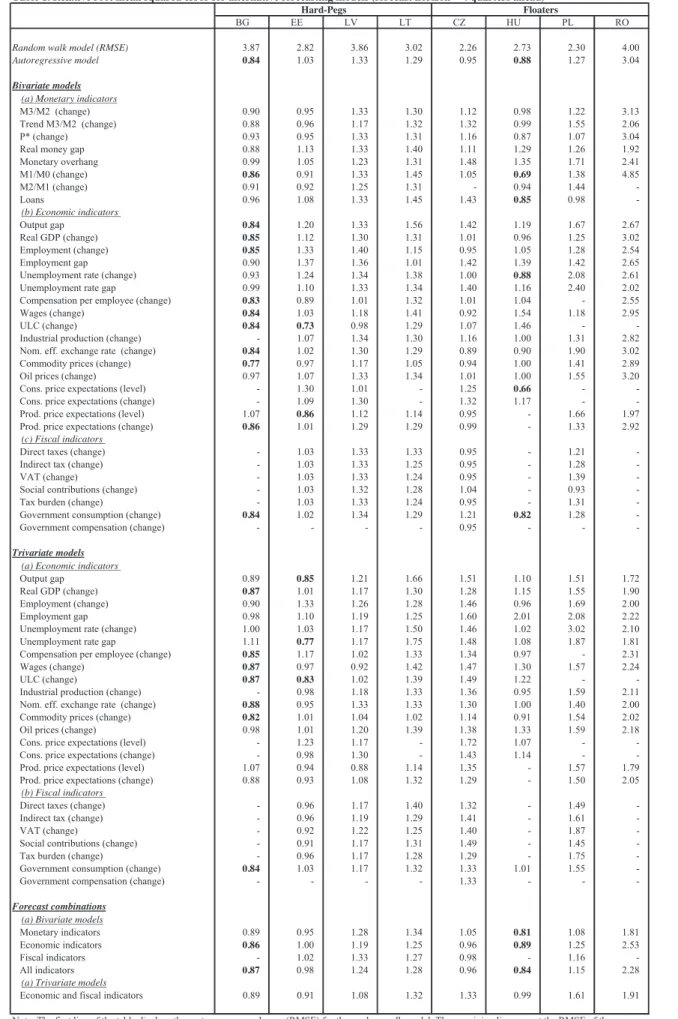
4.1 Short-term forecast of inflation developments (4 quarters ahead)

Following the methodology described in Section 3.2, Table 1 displays the absolute RMSE for

the RW as well as the values of the RMSEs of the different models relative to the RW. Hence,

relative RMSEs smaller than unity correspond to models outperforming the RW. When marked bold, relative RMSEs smaller than unity correspond to models that significantly outperform the RW (by reference to a Diebold-Mariano test).

Looking at Table 1, the results show that at the 4-quarter horizon the bivariate and trivariate (two-pillar Phillips curve) models perform worse than the RW benchmark in all countries but Bulgaria, Estonia and Hungary. This confirms that at the short-term horizon it is difficult to improve the forecast performance upon this simple RW benchmark. In the three countries where either bivariate or trivariate (two-pillar Philipps curve) models are able to significantly outperform the RW, it appears that different factors can help explaining inflation developments as indicated by the best-performing models.

x In Bulgaria the bivariate model with commodity price inflation performs best, possibly

reflecting the relatively large weight of food and energy prices in the consumer’s basket of this economy. The bivariate model with growth of compensation per employee and the trivariate (two-pillar Phillips curve) model with trend M3 growth and commodity price inflation also significantly outperform the RW and to a lesser extent also improve upon the AR model.

x In Estonia the bivariate model with ULC growth performs best. The bivariate model

with producers' price expectations also performs significantly better than either the RW or the AR model (the latter performs worse than the RW for Estonia). In addition, the trivariate (two-pillar Phillips curve) models with the output gap, the unemployment gap and ULC growth perform better than the RW. With the exception of ULC growth, these trivariate (two-pillar Phillips curve) models perform better than the bivariate models with these economic variables, which suggests that combining a monetary indicator (here: trend M2 growth) with economic indicators in some cases improves forecast accuracy.

x In Hungary the bivariate models with consumers’ price expectations and M1 growth

perform best. Both models display considerably better forecasting performance than the AR model, which itself performs significantly better than the RW. The bivariate

models with loan growth, the change in the unemployment rate and government consumption growth also perform significantly better than the RW even though the improvement upon the AR model is not very sizeable. Interestingly, Hungary with its high and rather volatile general government deficit is among the few countries for which we find that fiscal policy has predictive power for inflation in the short run.

As regards the forecast combinations at the 4-quarter horizon, they are not able to significantly outperform the RW forecast in any NMS apart from Bulgaria and Hungary. In Hungary, the combined forecast of monetary indicators performs the best among these combined forecasts.

Overall, we find that when trying to forecast inflation developments at the 4-quarter horizon, in the few countries in which we find models performing significantly better than the RW, the best performing models are bivariate models with economic indicators. In Estonia and Bulgaria some labour market indicators seem to be particularly capable to outperform the RW. This may broadly reflect a labour market tightening over the sample period in these fast growing and at times overheating economies.

Table 1. Relative root mean squared error for alternative forecasting models (forecast horizon = 4 quarters ahead)

BG EE LV LT CZ HU PL RO

Random walk model (RMSE) 3.87 2.82 3.86 3.02 2.26 2.73 2.30 4.00 Autoregressive model 0.84 1.03 1.33 1.29 0.95 0.88 1.27 3.04

Bivariate models

(a) Monetary indicators

M3/M2 (change) 0.90 0.95 1.33 1.30 1.12 0.98 1.22 3.13

Trend M3/M2 (change) 0.88 0.96 1.17 1.32 1.32 0.99 1.55 2.06

P* (change) 0.93 0.95 1.33 1.31 1.16 0.87 1.07 3.04

Real money gap 0.88 1.13 1.33 1.40 1.11 1.29 1.26 1.92

Monetary overhang 0.99 1.05 1.23 1.31 1.48 1.35 1.71 2.41 M1/M0 (change) 0.86 0.91 1.33 1.45 1.05 0.69 1.38 4.85 M2/M1 (change) 0.91 0.92 1.25 1.31 - 0.94 1.44 Loans 0.96 1.08 1.33 1.45 1.43 0.85 0.98 (b) Economic indicators Output gap 0.84 1.20 1.33 1.56 1.42 1.19 1.67 2.67 Real GDP (change) 0.85 1.12 1.30 1.31 1.01 0.96 1.25 3.02 Employment (change) 0.85 1.33 1.40 1.15 0.95 1.05 1.28 2.54 Employment gap 0.90 1.37 1.36 1.01 1.42 1.39 1.42 2.65

Unemployment rate (change) 0.93 1.24 1.34 1.38 1.00 0.88 2.08 2.61

Unemployment rate gap 0.99 1.10 1.33 1.34 1.40 1.16 2.40 2.02

Compensation per employee (change) 0.83 0.89 1.01 1.32 1.01 1.04 - 2.55

Wages (change) 0.84 1.03 1.18 1.41 0.92 1.54 1.18 2.95

ULC (change) 0.84 0.73 0.98 1.29 1.07 1.46 -

Industrial production (change) - 1.07 1.34 1.30 1.16 1.00 1.31 2.82

Nom. eff. exchange rate (change) 0.84 1.02 1.30 1.29 0.89 0.90 1.90 3.02

Commodity prices (change) 0.77 0.97 1.17 1.05 0.94 1.00 1.41 2.89

Oil prices (change) 0.97 1.07 1.33 1.34 1.01 1.00 1.55 3.20

Cons. price expectations (level) - 1.30 1.01 - 1.25 0.66 -

Cons. price expectations (change) - 1.09 1.30 - 1.32 1.17 -

Prod. price expectations (level) 1.07 0.86 1.12 1.14 0.95 - 1.66 1.97

Prod. price expectations (change) 0.86 1.01 1.29 1.29 0.99 - 1.33 2.92

(c) Fiscal indicators

Direct taxes (change) - 1.03 1.33 1.33 0.95 - 1.21

Indirect tax (change) - 1.03 1.33 1.25 0.95 - 1.28

VAT (change) - 1.03 1.33 1.24 0.95 - 1.39

Social contributions (change) - 1.03 1.32 1.28 1.04 - 0.93

Tax burden (change) - 1.03 1.33 1.24 0.95 - 1.31

Government consumption (change) 0.84 1.02 1.34 1.29 1.21 0.82 1.28

Government compensation (change) - - - - 0.95 - -

-Trivariate models

(a) Economic indicators

Output gap 0.89 0.85 1.21 1.66 1.51 1.10 1.51 1.72

Real GDP (change) 0.87 1.01 1.17 1.30 1.28 1.15 1.55 1.90

Employment (change) 0.90 1.33 1.26 1.28 1.46 0.96 1.69 2.00

Employment gap 0.98 1.10 1.19 1.25 1.60 2.01 2.08 2.22

Unemployment rate (change) 1.00 1.03 1.17 1.50 1.46 1.02 3.02 2.10

Unemployment rate gap 1.11 0.77 1.17 1.75 1.48 1.08 1.87 1.81

Compensation per employee (change) 0.85 1.17 1.02 1.33 1.34 0.97 - 2.31

Wages (change) 0.87 0.97 0.92 1.42 1.47 1.30 1.57 2.24

ULC (change) 0.87 0.83 1.02 1.39 1.49 1.22 -

Industrial production (change) - 0.98 1.18 1.33 1.36 0.95 1.59 2.11

Nom. eff. exchange rate (change) 0.88 0.95 1.33 1.33 1.30 1.00 1.40 2.00

Commodity prices (change) 0.82 1.01 1.04 1.02 1.14 0.91 1.54 2.02

Oil prices (change) 0.98 1.01 1.20 1.39 1.38 1.33 1.59 2.18

Cons. price expectations (level) - 1.23 1.17 - 1.72 1.07 -

Cons. price expectations (change) - 0.98 1.30 - 1.43 1.14 -

Prod. price expectations (level) 1.07 0.94 0.88 1.14 1.35 - 1.57 1.79

Prod. price expectations (change) 0.88 0.93 1.08 1.32 1.29 - 1.50 2.05

(b) Fiscal indicators

Direct taxes (change) - 0.96 1.17 1.40 1.32 - 1.49

Indirect tax (change) - 0.96 1.19 1.29 1.41 - 1.61

VAT (change) - 0.92 1.22 1.25 1.40 - 1.87

Social contributions (change) - 0.91 1.17 1.31 1.49 - 1.45

Tax burden (change) - 0.96 1.17 1.28 1.29 - 1.75

Government consumption (change) 0.84 1.03 1.17 1.32 1.33 1.01 1.55

Government compensation (change) - - - - 1.33 - -

-Forecast combinations

(a) Bivariate models

Monetary indicators 0.89 0.95 1.28 1.34 1.05 0.81 1.08 1.81

Economic indicators 0.86 1.00 1.19 1.25 0.96 0.89 1.25 2.53

Fiscal indicators - 1.02 1.33 1.27 0.98 - 1.16

All indicators 0.87 0.98 1.24 1.28 0.96 0.84 1.15 2.28

(a) Trivariate models

Economic and fiscal indicators 0.89 0.91 1.08 1.32 1.33 0.99 1.61 1.91

Hard-Pegs Floaters

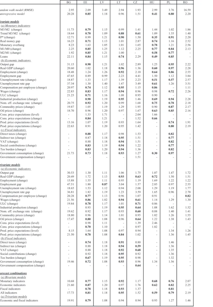
4.2 Long-term forecast of inflation developments (12 quarters ahead)

Looking at Table 2, it emerges that when forecasting 12-quarter ahead inflation dynamics in the NMS, an improved performance vis-à-vis the RW benchmark may be obtained in many of these countries when the information from monetary and non-monetary (economic and fiscal) indicators is taken into account. The main exceptions would be Bulgaria and Romania, but as discussed below the results for these countries should be taken with a grain of salt. Interestingly, the findings suggest that monetary indicators perform particularly well at the 12-quarter horizon across all other NMS. Turning first to the group of countries with a fixed exchange rate regime, the findings reveals the following:

x Specifically, in Estonia the bivariate model with trend M2 growth appears to perform

best. Although, all in all, 6 monetary bivariate models, 7 economic bivariate models and 4 fiscal bivariate models significantly outperform the RW benchmark, none of them significantly outperform the bivariate model with trend M2 growth. Five trivariate (two-pillar Phillips curve) models significantly outperform the RW model, but only one (the one with the tax burden change) does marginally better than the bivariate model with trend M2 growth, hence suggesting that adding a third variable to a model with lagged inflation and trend M2 growth does not noticeably improve upon the forecast performance of the latter.

x In Latvia, the trivariate (two-pillar Phillips curve) model with employment gap

performs best. At the same time, however, this is the only model significantly outperforming the RW.

x In Lithuania, the bivariate model with loan growth performs best at the 12-quarter

horizon. Moreover, both the bivariate model with trend M3 growth and the P* model perform better than the RW and AR models. In addition, 5 bivariate models with economic indicators, 5 bivariate models with fiscal indicators and 10 trivariate (two-pillar Phillips curve) models significantly outperform the RW but do not improve upon the forecasts of the bivariate model with loan growth.

x As already mentioned, for Bulgaria, there is not a single model outperforming the RW

at the 12-quarter horizon. However, this result is distorted by the inclusion of the 1990s in the regression sample, a period still characterised by hyperinflation in this country. This is clearly reflected in the AR model, the forecasting performance of which is worse than that of the RW by a factor of 20. If the regression sample start were instead set to 2000Q2 to exclude the volatile 1990s (which comes at the cost of a short evaluation sample), then a number of models with monetary and economic

indicators would improve upon the RW. The main message of this exercise is that for true out-of-sample forecasts (say 12-quarter ahead forecasts made in 2008Q3) there should be models that significantly improve upon the forecasts of the simple RW. However, in this paper we have chosen to adopt the same approach across countries in order to ensure equal treatment and comparability of results.

In the remaining countries, i.e. “the floaters”, a similar picture emerges.

x In the Czech Republic, the bivariate model with trend M2 growth performs best.

Moreover, nine trivariate (two-pillar Phillips curve) models also significantly outperform the RW, but only two (the ones with changes in indirect taxation and the nominal effective exchange rate) do marginally better than the bivariate model with trend M2 growth.

x In Hungary, the bivariate model with growth in government consumption performs the

best, yet only marginally better than the model with the P-star monetary indicator. These are the two single models that outperform the forecast of a simple AR model.

x As regards Poland, the bivariate model with the unemployment rate gap performs the

best at the 12-quarter horizon, followed by the bivariate model with wage growth. The finding that fiscal indicators work well compared to other countries may be related to the fact that Poland enacted several tax- and benefit reforms with a view to increasing labour supply and implemented a funded pension pillar.

x Finally, in Romania the only model able to significantly outperform the RW

benchmark is the trivariate (two-pillar Phillips curve) model with growth in compensation per employee. In general, the forecast performance of all models (including the RW) is very weak, which – as in the case of Bulgaria – reflects the fact that the economic environment was still quite unstable in the second half of the 1990s. As for Bulgaria, choosing the regression sample to start two years later (2000Q2) reveals that many models would significantly outperform the RW, a finding that may be useful for future forecasts of inflation for Romania.

As regards combined inflation forecasts for the 12-quarter horizon, most combined forecasts significantly outperform the RW benchmark in four countries (Estonia, Lithuania, Hungary and Poland) but not the respective best performing bivariate model in each of these countries. From these results one can conclude that over the long-term (12-quarter ahead) forecast horizon the role played by monetary factors in driving inflation dynamics does not differ substantially between the NMS with a “hard peg” and those with a floating exchange rate

regime. In particular, monetary indicators appear to become important variables to explain inflationary trends across the majority of the NMS. Compared to the short-term inflation dynamics, fiscal indicators also seem to play a more prominent role over the longer term. For example, in Hungary the best-performing model over the 12-quarter horizon is the bivariate model with government consumption; in Estonia and the Czech Republic the bivariate models with fiscal indicators also perform rather well. This may be explained by the fact that some fiscal policy measures may take time before they change the structure of the economy and take effect on inflation.

Table 2. Relative root mean squared error for alternative forecasting models (forecast horizon = 12 quarters ahead)

BG EE LV LT CZ HU PL RO

Random walk model (RMSE) 2.95 2.09 3.49 2.94 1.93 2.99 3.76 16.59 Autoregressive model 20.28 0.85 1.18 0.96 1.51 0.41 0.80 2.20

Bivariate models

(a) Monetary indicators

M3/M2 (change) 11.73 0.79 1.15 0.99 1.41 1.44 1.02 1.86

Trend M3/M2 (change) 18.64 0.70 1.09 0.88 0.61 1.09 1.35 1.40

P* (change) 12.71 0.99 1.21 0.90 1.50 0.35 0.91 2.20

Real money gap 16.23 0.71 1.13 1.01 2.87 0.74 1.16 2.52

Monetary overhang 8.23 1.63 1.05 1.01 1.65 0.78 1.21 2.56 M1/M0 (change) 2.25 0.85 1.25 1.12 2.25 0.77 0.84 2.13 M2/M1 (change) 1.92 0.85 1.21 1.00 - 0.58 0.77 Loans 22.11 0.84 1.15 0.74 2.29 0.49 0.85 (b) Economic indicators Output gap 31.15 0.90 1.21 1.02 2.89 1.25 0.95 2.22 Real GDP (change) 20.60 1.02 1.18 0.96 1.36 0.60 0.97 2.28 Employment (change) 18.48 1.24 1.26 0.92 2.10 0.64 0.86 2.55 Employment gap 47.65 0.89 0.99 2.23 4.41 1.50 1.12 3.84

Unemployment rate (change) 18.87 1.33 1.17 1.39 2.23 0.51 0.57 2.57

Unemployment rate gap 37.34 1.30 1.40 1.47 3.49 0.61 1.26 3.51

Compensation per employee (change) 20.97 0.74 1.12 0.95 1.15 0.86 - 1.11

Wages (change) 22.83 0.83 1.17 0.94 0.96 0.98 0.72 2.26

ULC (change) 21.23 0.71 1.16 1.08 0.95 0.90 -

Industrial production (change) - 0.90 1.19 0.95 1.46 0.69 0.94 2.28

Nom. eff. exchange rate (change) 20.75 0.92 1.20 0.99 1.68 0.75 0.78 2.18

Commodity prices (change) 19.87 1.05 1.19 1.29 1.95 0.90 0.87 2.17

Oil prices (change) 18.70 0.96 1.20 0.97 1.67 0.63 0.85 2.16

Cons. price expectations (level) - 1.33 1.71 - 2.04 1.66 -

Cons. price expectations (change) - 0.84 1.21 - 1.52 0.66 -

Prod. price expectations (level) 13.16 1.07 1.19 0.93 1.64 - 0.74 1.91

Prod. price expectations (change) 22.63 0.91 1.20 0.95 1.42 - 0.80 2.19

(c) Fiscal indicators

Direct taxes (change) - 0.88 1.17 0.98 1.53 - 0.82

Indirect tax (change) - 0.87 1.18 0.95 1.51 - 0.77

VAT (change) - 0.88 1.18 0.94 1.51 - 0.82

Social contributions (change) - 0.83 1.19 0.94 1.22 - 0.77

Tax burden (change) - 0.83 1.20 0.94 1.36 - 0.82

Government consumption (change) 21.73 0.73 1.18 0.93 1.27 0.30 0.97

Government compensation (change) - - - - 1.51 - -

-Trivariate models

(a) Economic indicators

Output gap 30.53 1.30 1.11 1.06 1.75 1.07 1.47 1.72

Real GDP (change) 20.49 1.72 1.13 0.93 0.63 0.72 1.50 1.51

Employment (change) 15.88 1.55 1.11 0.95 1.19 1.69 1.22 1.22

Employment gap 47.51 1.80 0.87 3.04 1.57 2.85 0.97 2.55

Unemployment rate (change) 18.65 1.53 1.12 0.94 2.08 1.29 1.19 1.77

Unemployment rate gap 36.81 1.82 1.19 1.23 3.59 1.65 0.96 2.70

Compensation per employee (change) 20.28 0.77 1.13 0.96 1.07 0.91 - 0.82

Wages (change) 21.56 0.86 1.02 0.94 0.61 1.14 1.29 1.30

ULC (change) 19.84 0.78 1.17 1.01 0.71 0.86 -

Industrial production (change) - 0.93 1.19 0.95 0.64 1.08 1.62 1.52

Nom. eff. exchange rate (change) 19.62 0.92 1.17 0.93 0.60 0.88 1.40 1.41

Commodity prices (change) 18.80 0.96 1.14 1.01 0.95 1.02 1.26 1.55

Oil prices (change) 17.47 0.80 1.08 0.96 0.64 1.22 1.38 1.43

Cons. price expectations (level) - 0.98 1.11 - 1.39 2.46 -

Cons. price expectations (change) - 0.70 1.10 - 0.97 1.02 -

Prod. price expectations (level) 8.15 1.64 1.08 0.97 0.94 - 1.34 1.26

Prod. price expectations (change) 21.50 0.78 1.08 0.84 1.02 - 1.36 1.45

(b) Fiscal indicators

Direct taxes (change) - 0.74 1.18 0.91 0.80 - 1.46

Indirect tax (change) - 0.88 1.18 0.94 0.59 - 1.36

VAT (change) - 0.88 1.18 0.92 0.68 - 1.35

Social contributions (change) - 0.92 1.18 0.95 0.92 - 1.36

Tax burden (change) - 0.67 1.19 0.95 0.98 - 1.32

Government consumption (change) 19.46 0.72 1.08 0.93 0.96 1.34 1.56

Government compensation (change) - - - - 0.64 - -

-Forecast combinations

(a) Bivariate models

Monetary indicators 10.68 0.77 1.15 0.92 1.17 0.68 0.76 2.07

Economic indicators 21.60 0.87 1.20 0.97 1.76 0.62 0.82 2.25

Fiscal indicators - 0.78 1.18 0.93 1.37 - 0.81

All indicators 17.73 0.81 1.18 0.95 1.52 0.59 0.79 2.19

(a) Trivariate models

Economic and fiscal indicators 19.91 0.79 1.08 0.94 0.94 0.93 1.27 1.46

Hard-Pegs Floaters

5. Conclusions

To the best of our knowledge, this paper is the first systematic study to analyse the performance of a large set of monetary, economic and fiscal indicators in explaining inflation dynamics in the NMS, including bivariate models and trivariate (two-pillar Phillips curve) models. Three findings can be highlighted.

First, the performance of the bivariate and trivariate (two-pillar Phillips curve) forecasting models differs substantially across countries in that different variables seem to be influencing to a different extent inflation developments at different horizons. This is likely to derive from the fact that, notwithstanding some similarities, economic structures and institutions do vary across the NMS.

Second, at the 4-quarter horizon, with the exception of Bulgaria, Estonia and Hungary, none of the bivariate and trivariate (two-pillar Phillips curve) forecasting models significantly outperform the RW model. This result echoes the findings of Stock and Watson’s (2008) recent literature review suggesting that inflation is hard to forecast in the U.S. and other OECD economies and that it is difficult to improve upon simple benchmark models. Overall, we find that when trying to forecast inflation developments at the 4-quarter horizon, in the few countries for which we find models performing better than the RW, such models are in general based on economic and fiscal indicators. In the hard peg countries Estonia and Bulgaria some labour market indicators seem to be particularly capable to forecast short-run inflation. This may reflect a labour market tightening over the sample period in these fast growing and at times overheating economies.

Third, at the 12-quarter horizon a number of bivariate and trivariate (two-pillar Phillips curve) forecasting models significantly outperform the forecasts of the RW model. In particular, monetary indicators do appear to contain useful information for predicting inflation at longer (3-year) horizons in these countries. Interestingly, the role played by monetary factors in driving inflation dynamics does not differ substantially between the NMS with a “hard peg” and those with a floating exchange rate regime. Thus, monetary indicators appear to become important variables to explain inflationary trends across the majority of the NMS over the long-term forecasting horizon.

References

Assenmacher-Wesche, K., and S. Gerlach (2007). Money at Low Frequencies. Journal of the

European Economic Association 5: 534–542.

Assenmacher-Wesche, K., and S. Gerlach (2008). Interpreting Euro Area Inflation at High

and Low Frequencies. European Economic Review 52: 964-986.

Benati, L. (2008). Money, Inflation and New Keynesian Models. ECB (mimeo).

Calza, A., D. Gerdesmeier and J. Levy (2001). Euro area money demand: measuring the

opportunity costs appropriately. IMF Working Paper No. 01/179.

Carstensen, K. (2007). Is Core Money Growth a Good and Stable Inflation Predictor in the Euro Area? Kiel Working Paper 1318.

Clark, T.E. and M.W. McCracken (2005). Evaluating Direct Multistep Forecasts.

Econometric Reviews 24: 369-404.

Dabusinskas, A. (2005). Money and Prices in Estonia. Bank of Estonia Working Paper 705. Darvas, Z. and G. Szapáry (2008). Euro Area Enlargement and Euro Adoption Strategies.

European Economy. Economic Papers 304, February 2008.

De Santis, R., C.A. Favero, B. Roffia (2008). Euro area money demand and international portfolio allocation: a contribution to assessing risks to price stability. ECB Working Paper No. 926.

Diebold, F.X., and R.S. Mariano (1995). Comparing Predictive Accuracy. Journal of Business

and Economic Statistics 13: 253-563.

Fischer, B., M. Lenza, H. Pill, and L. Reichlin (2006). Money and Monetary Policy: The ECB

Experience 1999-2006. Paper presented at the 4th ECB Central Banking Conference.

Frankel, Jeffrey (2006). The Effect of Monetary Policy on Real Commodity Prices. In John

Campbell (Editor). Asset Prices and Monetary Policy. University of Chicago Press.

Gerlach, S. (2003). The ECB’s Two Pillars. CEPR Discussion Paper 3689.

Gerlach, S. (2004). The Two Pillars of the European Central Bank. Economic Policy 40:

389-439.

Hofmann, B. (2008). Do Monetary Indicators Lead Euro Area Inflation? ECB Working Paper 867.

Hubrich, K. (2005). Forecasting euro area inflation: Does aggregating forecasts by HICP

component improve forecast accuracy?. International Journal of Forecasting 21: 119-136.

Kamps, C., N. Leiner-Killinger and R. Martin (2009) The Cyclical Impact of EU Cohesion

Policy in Fast Growing EU Countries, Intereconomics, forthcoming.

Kotlowski, J. (2005), Money and Prices in the Polish Economy: Seasonal Cointegration Approach, Warsaw School of Economics, Dept. of Applied Econ. Working Paper 3-05.

Lucas, Robert E., Jr. (1996). Nobel Lecture: Monetary Neutrality. Journal of Political

Economy 104: 661-682.

Nicoletti-Altimari, S. (2001). Does Money Lead Inflation in the Euro Area? ECB Working Paper 63.

Orphanides, A. (2008). Taylor Rules. In S.N. Durlauf and L.E. Blume (Editors). The New

Stock, J., and M. Watson (1999). Forecasting Inflation. Journal of Monetary Economics 44: 293-335.

Stock, J., and M. Watson (2007). Why Has U.S. Inflation Become Harder to Forecast?

Journal of Money, Credit and Banking 39: 3-33.

Stock, J., and M. Watson (2008). Phillips Curve Inflation Forecasts. NBER Working Paper 14322. Cambridge, MA.

Taylor, J.B. (1993). Discretion versus Policy Rules in Practice. Carnegie-Rochester