Loyola University Chicago
Loyola University Chicago
Loyola eCommons
Loyola eCommons
Computer Science: Faculty Publications and
Other Works
Faculty Publications
2017
Queryable Compression for Massively Streaming Social Networks
Queryable Compression for Massively Streaming Social Networks
Chandra N. Sekharan
Sridhar Radhakrishnan
University of Oklahoma Norman Campus
Ben Nelson
University of Oklahoma
Amlan Chatterjee
California State University, Dominguez Hills
Follow this and additional works at: https://ecommons.luc.edu/cs_facpubs Part of the Computer Sciences Commons
Recommended Citation
Recommended Citation
Sekharan, Chandra N.; Radhakrishnan, Sridhar; Nelson, Ben; and Chatterjee, Amlan. Queryable
Compression for Massively Streaming Social Networks. , , : , 2017. Retrieved from Loyola eCommons, Computer Science: Faculty Publications and Other Works,
This Technical Report is brought to you for free and open access by the Faculty Publications at Loyola eCommons. It has been accepted for inclusion in Computer Science: Faculty Publications and Other Works by an authorized administrator of Loyola eCommons. For more information, please contact [email protected].
Queryable Compression on Streaming Social
Networks
Michael Nelson & Sridhar Radhakrishnan
School of Computer ScienceUniversity of Oklahoma Norman, OK, USA
{Michael.A.Nelson-1, sridhar}@ou.edu
Amlan Chatterjee
Department of Computer Science California State University Dominguez HillsCarson, CA, USA [email protected]
Chandra N. Sekharan
Department of Computer ScienceLoyola University Chicago Chicago, IL, USA [email protected]
Abstract—The social networks of today are a set of massive, dynamically changing graph structures. Each of these graphs contain a set of nodes (individuals) and a set of edges among the nodes (relationships). The choice of representation of a graph determines what information is easy to obtain from it. However, many social network graphs are so large that even their basic representations (e.g. adjacency lists) do not fit in main memory. Hence an ongoing field of study has focused on designing compressed representations of graphs that facilitate certain query functions.This work is based on representing dynamic social networks that we call streaming graphs where edges stream into our compressed representation.
The crux of this work is the use of a novel data structure for streaming graphs that is based on an indexed array of compressed binary trees that builds the graph directly without using any temporary storage structures. We provide fast access methods for edge existence (does an edge exist between two nodes?), neighbor queries (list a node’s neighbors), and streaming operations (add/remove nodes/edges). We test our algorithms on public, anonymized, massive graphs such as Friendster, LiveJournal, Pokec, Twitter, and others. Our empirical evaluation is based on several parameters including time to compress, memory required by the compression algorithm, size of compressed graph, and time to execute queries. Our experimental results show that our current approach outperforms previous approaches in various key respects such as compression time, compression memory, compression ratio, and query execution times and hence the best to date overall.
Index Terms—Graph Compression, Binary Tree, Online Social Networks, Streaming Graphs
I. INTRODUCTION
Given a social network, it can be represented as a graph
G = (V, E), where V is a set of nodes (individuals) and
E is a set of edges (relationships). Most social networks like Facebook are undirected, meaning that the relationship is automatically reciprocated. In contrast, a social network like Twitter is directed, as meant by their concept of ’following’. Clearly, we can see that knowledge learned from these graphs is beneficial, as it may help to better coordinate events, suggest friends, advertise, and recommend games.
Social networks are ever growing. For example, from De-cember 2014 to March 2015, the number of daily active Facebook users grew from 890 million to 963 million [1]. Social networks are not limited to the number of people in the world, since entities such as companies and communities may
form an account as a new node. Clearly, such large, streaming graphs present a challenge to social network analysis.
Many different queries may be run on social networks. When developing a queryable compression technique, the compressed structure is usually designed to be efficient with a specific set of queries [7]. The most popular of these are arguably community operations and the reachability query. When building the algorithms used to answer these queries, the neighbor enumeration and edge existence operations are put to heavy use. This is true for many other classes of problems, including network pattern mining and friend suggestion.
Consider our Friendster snapshot withn= 65608366nodes andm= 1806067135edges. Using a boolean adjacency ma-trix representation, we get a size of656083662 bits = 538TB. Assuming 64-bit pointers and an adjacency list representation the memory needed can be estimated to be about 41 gigabytes which exceeds the typical RAM size of most computers. Queries such as neighbor enumeration and edge existence can be time-consuming in such high memory environments. These queries have time complexities ofO(n)andO(1), respectively, on the adjacency matrix and O(σ(n))on the adjacency lists, where σ(n)) is the degree of the graph. However, if the structure does not fit in memory it must make access calls to disk, which incur a high time penalty. Given this, our desire is to compress the graph to a size that can fit in the main memory but also provide mechanisms to perform neighbor and edge queries directly on the compressed structure. It is worth pointing out that for graphs represented in distributed memories, our compression techniques can be easily extended. Most raw, uncompressed graphs are downloaded from vari-ous sources as plain text files. These files are merely the graph in edge list form. That is, each line consists of two numbers,u
andv, separated by a space. A common requirement for most compression algorithms is an intermediate structure, such as an adjacency list, that is built from this edge list and used to efficiently build a final compressed structure [10]. Since we can incrementally build our compression, we do not require such an intermediate structure.
For obvious reasons, the original edge list text files are stored with common compression programs such as gzip. For large graphs like our Friendster graph, this is at least 41GB of necessary memory just in the preprocessing stage.
In this paper, we also present a method of compressing the graph directly from its gzipped edge list format. Since our compression scheme uses no intermediate structure when compressing, this ensures minimal memory overhead.
As previously mentioned, social networks are dynamic due to constantly changing user base or changing relationships. Hence our approach is to have a structure which can modify the compressed graph as edges and nodes are added and removed.
Social network graphs and their queries are node-centric, as evidenced by the popularity of the neighbor query. Our novel compression technique is based on indexed arrays of compressed binary trees. The binary trees will be responsible for compressing a node’s edges, and the indexes will provide quick access to those nodes in the compressed graph. Our motivation for using binary trees is an extension from our work with the quadtree data structure [12]. The quadtree structure in our previous work could be thought of as compressing the graph’s entire 2d adjacency matrix representation, whereas the present approach compress the individual rows of the matrix into binary trees, exploiting the node-centric nature of queries. This allows for increased query efficiency.
Our contributions can be summed up as:
• We introduce the indexed array of binary trees data structure that incrementally constructs the compressed file as nodes and edges are added and removed (streaming graph model). Existing algorithms require an intermedi-ate representation (e.g.,adjacency list or matrix) before compression.
• We have provided a method of compressing the graph directly from its gzipped edge list form.
• We have developed algorithms for edge and neighbor queries that directly operate on the compressed file. • A detailed empirical study is also presented that uses
the SNAP database [14] to obtain data on several social networks. The compressed output is directly created from the SNAP data sets that are in edge list format . • Comparison with state-of-the-art techniques including
Backlinks compression and Slashburn compression re-veals that our approach is superior in many respects such as compression time, compression memory, and query execution times. The compression ratios of the datasets using our algorithms are smaller than Backlinks [4] and Slashburn [9] which is to be expected because of the data being streamed in incrementally as opposed to being available in its entirety. Our present technique improves the compression ratio from our previous work [12] and results in better query times. Keeping in mind the inherent challenges in the streaming graphs model for compression and query times, we believe our present approach is overall the best to date.
The rest of the paper is organized as follows. In Section II, we review related work and show that all existing work is based on the availability of the entire adjacency matrix or list for compression to complete. In Section III, we formally define our queries and review common social network graph
terms. Our new binary tree compression is introduced and described in Section IV. We report empirical results in Section V. Finally, we conclude the paper in Section VI.
II. RELATEDWORK
Social network compression is preceded by the more general case of web graph compression. In such a case, the web pages are vertices and hyperlinks are directed edges. While we believe that we are the first ones to provide a compression technique for streaming graphs that supports the same query operations as we do, there are several existing works that have similar compression algorithms that are worth noting.
Adler and Mitzenmacher [2] introduced a web graph com-pression scheme by finding nodes with similar sets of neigh-bors. Randall et al. [13] were the first to use the lexicographical ordering of a web pages URL to compress a graph. Their method exploits the fact that many pages on a common host have similar sets of neighbors. Boldi and Vigna [3] continued taking advantage of properties of web graphs in lexicographical ordering. They found that proximal pages in URL lexicographical ordering often have similar neighbor-hoods. This lexicographical locality property allowed them to use gap encodings when compressing edges. In order to further improve compression, Boldi et al. [3] developed new orderings that combine host information and Gray/lexicographic order-ings.
In 2009, Chierichetti et al. [4] modified the Boldi and Vigna [3] compression method to better target social networks. Their method exploits the similarity and locality properties of web pages along with the idea that social networks have a high number of reciprocal edges. This method is called the Backlinks Compression scheme.
In 2014, Liakos et al. [8] also improved Boldi-Vigna’s compression ratio and access times by separately compressing the dense main diagonal stripe of the graph’s adjacency matrix. In 2010, Maserrat and Pei [11] introduced a compression scheme specifically designed to compress social networks while maintaining sublinear neighbor queries. They achieve this by implementing a novel Eulerian data structure using multi-position linearization. Their results are the first to answer out-neighbor and in-neighbor queries in sublinear time.
In 2014, Lim et al [9] invented Slashburn, a new ordering method to run on the graph before a general compression. The idea is to stray away from the definition of ‘caveman’ communities and instead use the idea of real world graphs being more like hubs and spoke connected only by the hubs. After running their ordering function, they use a block-wise encoding method (such as gzip) for the actual compression. The technique described in Slahburn [9] is novel that reduces the total number of blocks (where a block is a sub-matrix with non-zero entries). Their query times focus more on the problem of matrix-vector multiplication, which is used in prob-lems such as PageRank, diameter estimation, and connected components [6].
This research was partly inspired by our previous work involving quadtree compression [12]. There we treated the
boolean adjacency matrix as a 2D space to be compressed by a quadtree. The resulting tree was outputted in BFS order as a string of bits. Like the method presented in this paper, the quadtree approach also was a compression that required no intermediate representation to compress. While the graph’s final compressed size was indeed comparable with existing compression standards, the query times were slower than desired. Our proposed approach overcomes this deficiency by (i) by following a node-centric compression scheme, and (ii) using an indexed array of compressed binary trees rather than a quad-tree. The work described here for streaming graphs achieves a degree of performance that, in most metrics of importance to compression, either meet or exceed previous results, especially query times. Our present work’s compression ratios turn out to be less than for the benchmarks we compared with, however, this is only due to the inherent difference in the model (streaming vs non-streaming).
III. PRELIMINARIES
In this section, we describe some social network char-acteristics, common operations, and standard compression techniques.
A. Social networks
Social networks (SN) are graphs wherein a node represents a person and an edge is a friendships between two people. Here we will describe the general characteristics that emerge in these types of graphs.
1) Sparseness: Most importantly, SNs are very sparse. This means that there are very few edges relative to the total number of possible edges. For example, our LiveJournal graph contains about 4.8 million nodes and about 69 million edges. The total number of possible edges is(4.8∗106)2= 2.3∗1013. Therefore we only have(100∗(6.9∗106)/(2.3∗1013) = 3∗10−5%of the total edges possible. If we were to draw the boolean adjacency matrix for this graph, it would be mostly zeros.
2) Similarity: This property states that nodes close to each other in a lexicographical ordering have similar sets of neighbors. For example, in a high school with 300 students, the nodes might be numbered 0−299 in a lexicographical ordering. Since the students are likely to be friends with each other, many of the nodes will have similar sets of neighbors. 3) Locality: Locality is tied closely with similarity, but the distinction is important. With locality, a node tends to be connected to other nodes closer to its position in the lexicographical ordering. In other words, node0is more likely to be connected to node 100rather than node 1000000. B. Social network compression
Next, we outline common compression exploits for the char-acteristics described in Section III-A. Our new compression technique doesn’t make explicit use of any of these exploits, but our benchmark compression and many other algorithms do. Regardless, these techniques are standard background knowledge when understanding any SN compression.
1) Gap encoding: This technique takes advantage of the locality property. Even though the label numbers for a node’s neighbors may be large, the numbers should be close to each other. Therefore instead of actually encoding the large label numbers, we encode the differences (gaps) between them. For example, if we have nodes labeled 1000000 and 1000001, instead of encoding these two large numbers, we can encode the difference between them,1.
2) Removing neighbor redundancies: Next, we exploit the similarity property. Since this property states that nodes close to each other in the ordering share common neighbors, we can see that those similar neighbors present redundant information that can be optimized out. When encoding a noden, we check
k of the previously encoded nodes for common neighbors. If a sufficiently similar node xis found, node nis compressed based onx.
It is important to realize the negative affect this technique has on access operators. Since we are linking nodes to previous nodes, we can form a chain references. Therefore, when querying a node, we may end up having to query all the nodes in the reference chain. This is also why streaming is usually impractical on such compression schemes. One edge update may cause a large chain of updates.
3) Node re-ordering: If the ordering of the nodes in the graph is random, then the previous two exploits will fail. Therefore, a common bit of preprocessing is to re-order the nodes in the input graph based on some ordering scheme. The standard is a BFS lexicographical re-ordering. Recently, there is also Slashburn - a SN specific, node re-ordering technique [9].
C. Social network operations
Lastly, we review the common operations performed on social network graphs.
1) Edge existence queries: The most basic of the operation is checking whether or not an edge exists between two nodes. More formally, given a graphG= (V, E)and an edge(u, v), determine if(u, v)E.
2) Node neighbor queries: As previously stated, neighbor queries are arguably the most important for SNs. Given a graph
G= (V, E)and a node u, list all the out-neighbors of u. For a SN query-able compression to be effective, it must be able to answer this query efficiently.
3) Edge addition/removal: This operation is available only in streaming graph compressions, otherwise known as incre-mental graph compressions. These compressions allow edges and nodes to be efficiently added and removed without having to completely re-compress the graph.
IV. INDEXED ARRAY OF COMPRESSED BINARY TREES Next, we move on to the description of our new compression technique. For every input graphG= (V, E), we assume that
E is sorted and nodes inV are labeled from0to|V| −1. We also assume that|V|is rounded up to the next power of two. This assumption is only necessary for a direct construction, rather than an incremental one.
A. Node-centric, indexed structures
As previously mentioned, SNs and their query operations are node-centric. This indicates that our compression method must also be node-centric. That is, our compression technique will compress one node at a time, in order. Compressing a node consists of compactly representing all the node’s neighbors in a meaningful way. After a node is compressed, it is now a string of bits which are simply appended onto the final bitstring.
A consequence of being node-centric is that when querying for an edge (u, v), we must start at the beginning of the compressed graph and read sequentially up to node u. A workaround for this is to include an array of indexes that point to the positions of every node in the compressed graph. This is a common practice and sacrifices minimal space for a great speed increase on queries [8]. In our case, the space require-ment is O(nlog(n)), yet we receive a time improvement of
O(n2).
B. Compressed binary trees
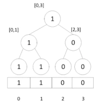
A binary tree is a tree in which every non-leaf node has a maximum of two children. A full binary tree of depth k has 2k leaf nodes. When a graphG= (V, E)is represented as a |V| × |V|boolean adjacency matrix, each rownof the matrix represents all the neighbors of noden. Knowing this, we can represent a matrix row of width|V|with a binary tree of depth
log2(|V|). This is shown in Figure 1.
Fig. 1:Binary tree from a row of an adjacency matrix
For a compressed binary tree, each node in the tree is encoded with one bit each. A node is set to true if it is a non-leaf node, or if it is a leaf node corresponding to an edge. All nodes marked false are leaf nodes. This encoding scheme prunes off sections of the matrix row that are empty, while the path to an edge must travel to the bottom of the tree. A compressed binary tree of Figure 1 is illustrated in Figure 2.
When a compressed binary tree is output to a bitstring, the graph is read in BFS order starting at the root. Therefore, the bitstring for the graph in 2 would be 11011. We can see that the row’s compression actually fails, since the row is not large and sparse enough. Figure 3 shows a compression that succeeds on a sparser adjacency row.
C. Analysis
Recall that a graph hasnnodes andmedges. Each edge is stored as a1in the boolean adjacency matrix, with the rest of
Fig. 2:A compressed binary tree from a row of an adjacency matrix
Fig. 3:A successful compression
the entries being 0. Given a binary tree mapped to a row of the matrix, a path to an edge has depthdlog2(n)e. Each node along this path requires 2 bits for its children, for a total of 2mdlog2(n)e+ 1. This is roughly twice thetheoretical lower
bound for representing all edges. However, most paths are going to share nodes in the upper levels of the binary tree. Maximizing the number of shared nodes is the purpose of node re-ordering.
We can see that the worst case results in a perfect binary tree, which is where all nodes have two children and all leaf nodes are at the same depth. This gives us 2n+1−1 nodes. These trees can formed from graphs such a complete graph or a graph such that every other edge (in the sorted order) is missing, such as the adjacency matrix in Figure 4. Here, we are given a boolean adjacency representation of a graph. Since it is checkered, there is no possible compression for this graph, and we are left with a perfect binary tree. There are other possible worst case graphs, but there can be no two edges missing,(un, vn)and(un+1, vn+1), such thatn is even. The parent node of those edges would become compressed, and we would no longer have a perfect binary tree. Since social network graphs are extremely sparse, they are far away from the worst case, as verified in Section V.
D. Direct construction
Since the input graph is usually a list of edges, there are two ways to compress. This first is to incrementally add (stream) each edge one at a time. This yields a time complexity of
O(mn), which is slow on graphs with a number of edges in the billions, especially due to the cost of the decompression
Fig. 4:A worst case adjacency matrix
step. A more interesting approach is to assume we are given all the edges at once. This way, we can achieve an initial compression with a time complexity of O(mlogn).
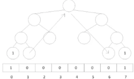
Using the assumption that edges are in order, we will show that each node’s compressed tree can actually be constructed left-to-right. Suppose that|V|= 8and that our input edge list consists only of(0,0)and(0,7). These edges are on opposite sides of each other in the binary tree for node 0. Notice that from these two edges, we can completely construct the final tree. This is because we know that everything between these two nodes should be set to false and pruned away. The parents of the edge nodes should obviously be set to true since they are non-leaf nodes. We know formally describe this process in Algorithm 1.
Algorithm 1: Binary tree compression
Input:A node’s sorted edge list
Output: The compressed node as a bitstring
1 begin
2 curP os←0;
3 foreach edge destination,v do
4 dcn←deepestCommonNode (curP os, v); 5 foreach node from curPos up to dcndo 6 color any right siblings as 0
7 color parent as 1
8 foreach node from dcndown to v do
9 color any left siblings as 0 10 color parent as 1
11 curP os←v
12 dcn←deepestCommonNode (curP os,n);
13 colordcn right child as 0; 14 return tree in BFS order;
DEFINITION- Deepest Common Node (DCN) - Given two leaf nodes in a binary tree,niandnj, the DCN is the deepest non-leaf node in the tree such that it lies on both ni’s and
nj’s paths to the root of the tree. For example, in Figure 1, the lead nodes for indexes1 and2have a DCN at the root.
In Algorithm 1, we can see that we are compressing one node at a time using the node’s sorted edge list. In Line 4, we calculate the deepest common node in the tree that the two edge nodes share. In Lines5through7, we traverse up to
the DCN between two leaf nodes, and set all parents to true and all siblings to false along the way. Similarly, in Lines 8 through 11, the same is done when traversing from the DCM to the second node. Lines12and13handle filling the rest of the tree, in case the last edge was not the rightmost node in the binary tree. This concept is further illustrated in Figure 5.
Fig. 5:Left-to-right compressed binary tree construction
Finally, we use Algorithm 1 to compress each node and then we store them in an indexed array. We describe this process in Algorithm 2. For our index’s integer encoding scheme, we use Delta Encoding [5].
Algorithm 2: Indexed array of binary trees compression
Input:The graph as a sorted edge list
Output: The compressed graph as a bitstring
1 begin
2 length← 0;
3 index←int[|V|];
4 foreach node,ndo
5 index[n]←length;
6 compressed[n]←CompressNode
(node.edges);
7 length+ =Delta(compressed[n].length) 8 return index + compressed;
Algorithm 2 loops through each node and uses Algorithm 1 to compress the node. While doing so, it also keeps track of the index position of the encoded node. Finally, it returns the list of indexes appended with the list of compressed nodes.
1) Proof of correctness:
Theorem:
Given a graph G= (V, E), Algorithm 2 provides a lossless compression ofG.
Proof:
Since Algorithm 2 already outputs a compressed version ofG, we must prove that this compression can be unambiguously reverted back to the original graph.
LetG0be the compressed version ofG. Then it is sufficient to show that givenG0, we can obtain the original edge listE
of the graphG.
Here we must make a note that the list of neighbors of each node is equivalent to E. That is, S|V|−1
u=0 (u, vN(u)) ≡ E, whereN(u)lists the neighbors ofu.
Therefore, since our compression simply compresses the neighbors of each node, it is sufficient to show that an arbitrary
compressed binary tree correctly stores the neighbors of the node it belongs to. In other words, we must prove that every edge destinationvappears as the appropriate leaf node inu0s
binary tree.
As before, let u be an arbitrary node and N(u) be the neighbors ofu. Clearly, rowuof the boolean adjacency matrix will contain10sfor each indexvN(u)and00sfor every other index in the row.
If we start at the root of the compressed binary tree, then that node represents indexes0through|V|−1of the adjacency matrix row. If the node is set to TRUE, then it has children to navigate to; i.e., the node leads to an edge. If it is set to
F ALSE, then it contains no children; i.e., it does not lead to an edge.
As we traverse through the left or right children, the range of indexes that the current node covers strictly decreases based on which child we navigated to. If we reach the maximum depth, the range of the current leaf node targets a single index of the adjacency matrix row. Since Algorithm 1 produces trees with leaf nodes only where the target index is vN(u), and Algorithm 2 uses it to actually compress the nodes, our compression is correct.
2) Compressing directly from a gzip compressed edge list: During our experiments, we encountered such large graphs that even the raw edge list format required over 30GB of RAM. Since most computers these days do not have access to large amounts of main memory, we devised a way to compress directly from a much smaller 8GB gzipped edge list. It is important to note that the gzipped file must also be sorted.
The technique is uses the zLib library that gzip is built on. This library allows us to partially inflate (decompress) the file in chunks. Since the file is sorted, we can decompress a single node before we re-compress it with our method. Obviously, this technique only affects compression time and memory required for compression. These differences are shown in V. E. Querying the compressed structure
We provide three operations that can be performed on our structure: checking edge existence, getting a node’s neighbors, and adding/removing edges. While these are all separate operations, they all involve knowing how to efficiently traverse the compressed tree in bitstring form.
Normally when traversing trees, the user has access to pointers. However, since this is a compressed tree, we must read bit-by-bit from left to right. We stored the tree as labels in BFS order, therefore we must start at the root and keep track of where in the tree we are as we traverse. As we do this, we must also make note of the next node in the tree we are interested in. In the next section, Algorithm 3 demonstrates this through the edge query.
1) Edge query: In this section, we present and describe the algorithm for checking edge existence in our structure. The process is formally given in Algorithm 3.
Algorithm 3 is an edge query, but it also represents the basics of traversing through our compressed tree. We can see thatbegCol andendColare the variables describing the node
Algorithm 3: Array of Binary Trees (ABT) Compression - Edge Query
Input:The compressed adjacnecy row as a bitstring, v
Output: True or False
1 begin
2 cur = 0, begCol = 0, endCol =n, nextIndex = 0,
nodesAtDepth = 1, nodesAtNextDepth = 0;
3 fori= 0;i <bitstring.Size();do 4 forj=i;j < nodesAtDepth;j+ +do
5 curN ode←bitstring.GetBit (j);
6 ifj==nextIndexthen
7 ifcurN ode== 1then
8 ifcurDepth==maxDepththen
9 return True;
10 midCol←(begCol+endCol)/2
11 pos←0 if y<midCol : else 1
12 nextIndex←i+nodesAtDepth+
nodesAtN extDepth+pos
13 ifposbegCol ←midCol else endCol
← midCol
14 nodesAtNextDepth += 2;
15 else ifcurN ode== 0then
16 return False;
17 else ifcurN ode== 1then
18 nodesAtNextDepth += 2;
19 i += nodesAtDepth;
20 nodesAtDepth = nodesAtNextDepth; 21 nodesAtNextDepth = 0;
currently being examined. Note that each non-leaf node in the binary tree represents a range of nodes as edge destinations in the graph. Leaf nodes have a range of size one, i.e., the actual edge.nextIndexis the position of the next node in the tree along the path to our edge. Keeping track of how many nodes in the current and next depths is crucial to calculating
nextIndex. The loop defined on Line 6 handles searching through each node in the current depth of the tree. Line 8 checks if the node currently being examined is the next node of interest on our path to the edge. If it is, Line 9 checks if the node is marked T rue and Line 10 tests if it is an edge node. Notice that we cannot return T rueuntil we have reached the bottom of the tree. In lines 13 and17, we increment nodesAtN extDepth by 2, since the presence of an uncompressed node indicates that its two children will be at the next depth.
2) Neighbor query: The neighbor query completely reads through the compressed tree, returning any leaf nodes set to true. By storing the positions and dimensions of multiple nodes, we can do this in one read.
3) Streaming edges: Adding an edge begins by finding the deepest node along its path that hasn’t been pruned off. Once we find the proper location, we build the rest of the path
by inserting the proper bits into the bitstring. If the edge to be added is close to an existing edge, the space added and execution time will be minimal. This process is formally described in Algorithm 4.
Removing an edge is the mirror of adding, but it still begins by finding the highest node in the path that it can compress. Then every bit representing nodes below it in the path are removed. Finally, the highest node is set to false. Compression benefits will be better the farther away the edge to be removed is from the other edges.
Algorithm 4: ABT Compression - Streaming an edge
Input:The compressed graph as a bitstring, x, y
1 begin
2 cur = 0, begCol = 0, endCol =n, nextIndex = 0, nodesAtDepth = 1, nodesAtNextDepth = 0;
3 fori= 0;i <bitstring.Size();do 4 forj =i;j < nodesAtDepth;j+ +do
5 curN ode← bitstring.GetBit(j);
6 if j==nextIndexthen
7 if curN ode== 1then
8 midCol←(begCol+endCol)/2
9 pos←0 if y<midCol : else 1
10 nextIndex←i+nodesAtDepth+
nodesAtN extDepth+pos
11 if posbegCol←midCol else endCol
←midCol
12 nodesAtNextDepth += 2;
13 else if curN ode== 0then
14 bitstring.SetBit (j, 1);
15 //Partially decompressj0s children all
the way to the leaf node for(x, y) return;
16 else if curN ode== 1then
17 nodesAtNextDepth += 2;
18 i += nodesAtDepth;
19 nodesAtDepth = nodesAtNextDepth; 20 nodesAtNextDepth = 0;
The beginning of Algorithm 4 is similar to the edge query in Algorithm 3. That is, it must first traverse through the tree to find the deepest compressed node that ranges over our edge. This first step completes at Line12, where we first come across a node of interest that is set to F alse. Immediately, the next thing to do is set this node toT rueas we are about to partially decompress it. A partial decompression means we only add children set to T rue on the path to our leaf node. All other children are left compressed and set to F alse. Since we are operating on a bitstring, this consists of inserting the nodes’ bits into their proper position.
V. EXPERIMENTS AND RESULTS
Our experiments involve running ABT compression and our benchmark Backlinks compression [4] on the datasets in Table I. Backlinks compression (BLC) was chosen as the benchmark compression since it is the state-of-the-art technique for social networks [8]. We have also compared the bits-per-edge of these two techniques against Slashburn compression [9] and reported the results in Table VIII. We chose to compare against Slashburn since they are technically a re-ordering algorithm that is subsequently compressed with gzip, which we also apply to our compressions as an additional step.
In this paper, we have set BLC to use BFS for the re-ordering algorithm and we have set the window size tok= 10. The datasets are stored as an edge list and the final output of the compressions is a bitstring.
We run all of our algorithms on a machine with an Intel(R) Xeon(R) CPU E5520 @ 2.27GHz (4 cores) with 64GB of RAM.
A. Compression
Our compression results in Table II provide a comparison among the original edge list file, our compression technique (ABT), Backlinks Compression (BLC), and the gzipped files of each.
When examining the initial compression sizes of ABT and BLC, it is clear that BLC outperforms ABT in terms of size. This is to be expected as ABT is a streaming compression. In order to allow a compressed structure to be easily query-able and modifiable, it must be slightly inflated. For example, the copy list technique used in BLC is one of the main reasons for their high compression rates. However, this is also the bottleneck for their slower query times and inability to stream edges. When a query or modification occurs on a node that copies its edges from achainof previous nodes, the operation may occur on each node in the chain.
BLC’s process of building copy lists is also one of the reasons why their compression times are so long. As previ-ously mentioned, we have set the window size to a common
k = 10. This means that we actually examine each node 10 times. Additionally, since BLC requires an adjacency list intermediate structure, the query times for that list also affect compression run times. ABT builds the structure directly from the edge list, therefore it compresses much faster.
Our reasoning for applying the additional gzip compression is a matter of in-memory querying vs storing on secondary memory. A non-gzipped compressed graph is easily queryable but takes up more memory. Once the user is done querying the graph, they may gzip the structure and store it in secondary memory.
As expected, gzipping ABT and BLC shrinks the size gap. This is best shown in the Friendster graph, where the gap shrinks from 2GB to 0.1GB. The best explanation for this occurrence is that ABT is more susceptible to gzip due to the runs of 0s indicating the compressed sections of the adjacency matrix rows.
TABLE I:The dataset stats
Directed? —V— —E— #Reciprocal Edges
Facebook FALSE 4039 88234 88234 Friendster FALSE 65608366 1806067135 1806067135 LiveJournal TRUE 4847571 68993773 26142536 LiveJournal(com) FALSE 3997962 34681189 34681189 NotreDame TRUE 325729 1497134 407026 Pokec TRUE 1632803 30622564 8320600 Twitter TRUE 81306 1768149 425853
TABLE II:Compressed graph sizes
.txt .txt.gz ABT ABT.gz BLC BLC.gz Facebook 835KB 214KB 96.45KB 82KB 110.32KB 93KB Friendster 31GB 8.2GB 7.7GB 5.3GB 5.7GB 5.2GB LiveJournal 1.1GB 248MB 224MB 168MB 139.98MB 122MB LiveJournal(com) 479MB 119MB 111.17MB 82MB 110.21MB 95MB Pokec 405MB 127MB 110.89MB 82MB 70MB 64.MB Twitter 20MB 6.1MB 4.8MB 3.7MB 3.3MB 3.1MB
Table II shows a comparison among the sizes of the raw graphs, our ABT compression, the BLC benchmark, and all of their respective gzipped files. The.txtfiles are the original edge list representations of the graphs. The.txt.gzare
those files after being gzipped.
TABLE III:Compression times
ABT BLC Facebook 0.32s 1.1s Friendster 4.1h 10h LiveJournal 8.6m 18.1m LiveJournal(com) 4.0m 11.4m Pokec 4.3m 8.9m Twitter 10.9s 26.3s
The data in Table III shows the total run time of both the ABT and BLC algorithms on each graph. Clearly, the run times depend on the size of the input graph.
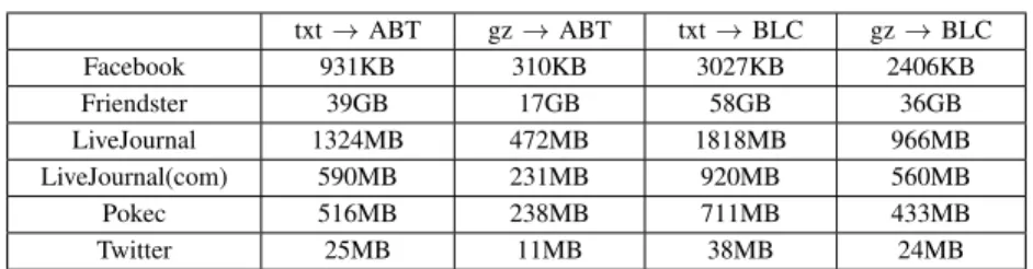
TABLE IV:Compression memory usage
txt→ABT gz→ABT txt→BLC gz→BLC Facebook 931KB 310KB 3027KB 2406KB Friendster 39GB 17GB 58GB 36GB LiveJournal 1324MB 472MB 1818MB 966MB LiveJournal(com) 590MB 231MB 920MB 560MB Pokec 516MB 238MB 711MB 433MB Twitter 25MB 11MB 38MB 24MB
In Table IV, we list the different memory requirements for running our algorithms. Not only does it show that ABT requires less memory than BLC, but it also shows the benefits of loading directly from a gzipped graph file.
TABLE V:Edge existence execution times ABT (ms) BLC (ms) Facebook 0.0008±0.0016 0.009±0.017 Friendster 0.0011±0.0026 0.037±0.091 LiveJournal 0.0002±0.0006 0.067±0.12 LiveJournal(com) 0.0003±0.0006 0.007±0.02 Pokec 0.0008±0.0016 0.011±0.0126 Twitter 0.0011±0.003 0.008±0.011
Table V shows the average edge query execution times, along with their standard deviation. All times are in milliseconds.
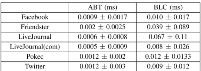
TABLE VI:Neighbor query execution times
ABT (ms) BLC (ms) Facebook 0.0009±0.0017 0.010±0.017 Friendster 0.002±0.0025 0.039±0.089 LiveJournal 0.0006±0.0008 0.067±0.11 LiveJournal(com) 0.0005±0.0009 0.008±0.026 Pokec 0.0012±0.002 0.012±0.0133 Twitter 0.0012±0.003 0.009±0.012
Table VI is the same as Table V, but for the neighbor query instead.
TABLE VII:Add edge execution times
ABT (ms) BLC (ms) Facebook 0.0052±0.012 -Friendster 0.012±0.073 -LiveJournal 0.0036±0.0088 -LiveJournal(com) 0.0028±0.0054 -Pokec 0.0064±0.017 -Twitter 0.0072±0.014
-Again, Table VII is the same as Table V but for streaming access times. Note that since BLC is not a streaming
compression, it does not have any entries.
TABLE VIII:Comparison with Slashburn graphs (bits-per-edge)
ABT ABT.gz BLC BLC.gz SB LiveJournal 26 19.5 16.2 14.15 16.5
Barabasi 17.2 8 20.8 13.36 8.5
Additionally, we provide Table VIII as a quick comparison with Slashburn [9]. The size metrics are in the traditional
bits−per−edge.
Next, we report that ABT uses much less memory during compression than BLC. This is obviously because ABT does not require an intermediate structure in order to efficiently compress. This benefit is massive, as many techniques are restricted to smaller graphs due to the larger graphs requiring too much memory. This fact, coupled with our new ability to also compress directly from the gzipped edge list file, guarantees minimal memory overhead.
Finally, since we use gzip to improve our results, we also include a compression comparison with Slashburn [9]. This is because Slashburn is technically a re-ordering algorithm that uses gzip to compress blocks in the adjacency matrix that formed as a result of the re-ordering. For the sake of consistency with Slashburn’s paper, we present the results using the traditionalbits-per-edgemetric.
B. Query operations
Our ABT structure facilitates two query operations, the edge query and the neighbor query. These are also the two queries supported by BLC.
Since both compression techniques are node-centric, we can use indexes for fast access to each node. For ABT, once the node of interest has been navigated to, we immediately begin reading the compressed tree. If it is an edge query, we stop when we find the edge, or when we find a compressed node that indicates that the edge does not exist. If it is instead a neighbor query, we must read the entire tree.
Similar to ABT, BLC may also use indexes to jump to the node being queried. However, the decoding process is more complicated than reading our simple tree. It not only involves
back tracing the copy lists, but also many integer decodings. Thus, on average, ABT outperforms BLC on both the edge and neighbor queries.
The neighbor query is essentially the same as the edge query for both ABT and BLC. Just as ABT requires the entire tree to be read, BLC requires that the entire adjacency list be read. Though again, BLC’s neighbor query suffers from the same problem that its edge query has with the copy lists. Therefore, since the queries are so similar, we can see that their access times are nearly identical but with higher variance.
C. Streaming operations
As described earlier, our compression method supports the streaming operation. That means that we are able to directly add/delete edges into the compressed structure without having to completely re-compress the graph. Conversely, BLC does not support this operation, mainly due to its incorporation of copy lists.
In Algorithm 4, we state that the streaming process is identical to the edge query operation. The only difference is that once we have navigated to the correct node, we may decompress or compress it by adding or removing the appropriate bits respectively.
By comparing Table V and Table VII, we see that although the edge query times are clearly faster that the streaming times, there is still a direct relationship between them. Since both operations navigate the tree in the same manner, the gaps between times are due to the actual cost of moving bits in the bitstring.
VI. CONCLUSIONS
In this paper, we have presented a novel, queryable, stream-ing social network compression usstream-ing an indexed array of compressed binary trees. We build this structure directly from the graph’s gzipped edge list text file without using any intermediate structure such as an adjacency list. These two techniques guarantee minimal memory overhead. Our compression also supports two queries, namely the edge and neighbor queries. Our approach facilitates the dynamic addition or removal of (streaming)edges from the compressed structure without having to completely re-compress the graph. We also provide various comparisons among our compres-sion, Backlinks [4] (as a benchmark), and Slashburn [9]. These comparisons use metrics such as compression size, time to compress, memory usage, and query times. Our basic query operations run, on average, 10 times faster than our BLC benchmark and our compression ratios exceed Slashburn compression. Because our technique is for streaming graphs, our compression ratios are less than BLC which is to be expected. Further work is being envisioned to improve the algorithms in [11], [9] using ideas presented in this work.
REFERENCES [1] http://www.cnbc.com/id/102610670, 2015.
[2] Micah Adler and Michael Mitzenmacher. Towards Compressing Web Graphs. InProceedings of the Data Compression Conference, DCC ’01, pages 203–212, Washington, DC, USA, 2001.
[3] P. Boldi and S. Vigna. The Webgraph Framework I: Compression Techniques. In Proceedings of the 13th International Conference on World Wide Web, WWW ’04, pages 595–602, New York, NY, USA, 2004. ACM.
[4] Flavio Chierichetti, Ravi Kumar, Silvio Lattanzi, Michael Mitzenmacher, Alessandro Panconesi, and Prabhakar Raghavan. On Compressing Social Networks. In Proceedings of the 15th ACM SIGKDD International Conference on Knowledge Discovery and Data Mining, KDD ’09, pages 219–228, New York, NY, USA, 2009. ACM.
[5] P Elias. Universal codeword sets and respresentations of the integers. In IEEE Transactions on Information Theory, pages 194–203, Piscataway, NJ, USA, 1975. IEEE Press Piscataway.
[6] U. Kang, Charalampos E. Tsourakakis, and Christos Faloutsos. PEGA-SUS: A Peta-Scale Graph Mining System Implementation and Observa-tions. InProceedings of the 2009 Ninth IEEE International Conference on Data Mining, ICDM ’09, pages 229–238, Washington, DC, USA, 2009. IEEE Computer Society.
[7] Chinmay Karande, Kumar Chellapilla, and Reid Andersen. Speeding Up Algorithms on Compressed Web Graphs. Internet Mathematics, 6(3):373–398, February 2009.
[8] Panagiotis Liakos, Katia Papakonstantinopoulou, and Michael Sioutis. Pushing the envelope in graph compression. CIKM ’14, pages 1549– 1558, November 2014.
[9] Yongsub Lim, U. Kang, and C. Faloutsos. SlashBurn: Graph Compres-sion and Mining beyond Caveman Communities. Knowledge and Data Engineering, IEEE Transactions on, 26(12):3077–3089, Dec 2014. [10] Sebastian Maneth and Fabian Peternek. A Survey on Methods and
Systems for Graph Compression. 6(3), 2015.
[11] Hossein Maserrat and Jian Pei. Neighbor Query Friendly Compression of Social Networks. In Proceedings of the 16th ACM SIGKDD International Conference on Knowledge Discovery and Data Mining, KDD ’10, pages 303–325, New York, NY, USA, 2010. Springiner-Verlag New York.
[12] Michael Nelson, Sridhar Radhakrishnan, Amlan Chatterjee, and Chandra Sekharan. On compressing massive streaming graphs with Quadtrees. InBig Data (Big Data), 2015 IEEE International Conference on, IEEE BigData ’15. IEEE Computer Society, 2015.
[13] Keith H. Randall, Raymie Stata, Janet L. Wiener, and Rajiv G. Wick-remesinghe. The Link Database: Fast Access to Graphs of the Web. InProceedings of the Data Compression Conference, DCC ’02, pages 122–131, Washington, DC, USA, 2002. IEEE Computer Society. [14] Stanford Network Analysis Project. Stanford Large Network Data