https://doi.org/10.1007/s10618-018-0560-3
Anomaly detection in spatiotemporal data via
regularized non-negative tensor analysis
Chaoguang Lin1 · Qiuhan Zhu1 · Shunan Guo1 · Zhuochen Jin1 · Yu-Ru Lin2 · Nan Cao1
Received: 17 November 2016 / Accepted: 15 March 2018 / Published online: 29 March 2018 © The Author(s) 2018
Abstract Anomaly detection in multidimensional data is a challenging task. Detect-ing anomalous mobility patterns in a city needs to take spatial, temporal, and traffic information into consideration. Although existing techniques are able to extract spa-tiotemporal features for anomaly analysis, few systematic analysis about how different factors contribute to or affect the anomalous patterns has been proposed. In this paper, we propose a novel technique to localize spatiotemporal anomalous events based on tensor decomposition. The proposed method employs a spatial-feature-temporal ten-sor model and analyzes latent mobility patterns through unsupervised learning. We first train the model based on historical data and then use the model to capture the anomalies, i.e., the mobility patterns that are significantly different from the normal patterns. The proposed technique is evaluated based on the yellow-cab dataset collected from New York City. The results show several interesting latent mobility patterns and traffic anomalies that can be deemed as anomalous events in the city, suggesting the effectiveness of the proposed anomaly detection method.
Keywords Tensor analysis · Anomaly detection · Outlier detection· Urban computing·Traffic analysis
Responsible editor: Jieping Ye.
B
Nan Cao[email protected] Yu-Ru Lin
1 Intelligent Big Data Visualization Lab, Tongji University, Shanghai, China 2 University of Pittsburgh, Pittsburgh, USA
1 Introduction
The high availability of transportation data such as taxi archives provides great opportunities for understanding people’s mobility patterns in a city. Despite the analysis performed for understanding the majority moving trend such as (Yuan et al. 2012), detecting and understanding regions with anomalous mobility pat-terns attract more and more attention especially in the big cities such as New York where traffic congestion is always a big transportation issue. Understand-ing those anomalous traffic patterns can help with a better management of the city.
The above problem lies in the domain of anomaly detection which has been exten-sively studied in the field of data mining and machine learning. Many techniques have been proposed (Chandola et al.2009) and applied to various application domains. How-ever most of the existing techniques fail to provide a clear decomposition of the data to reveal the potential factors that best capture, describe, or affect the anomalous behav-iors. These factors are usually critical for the interpretation of the analysis results and can be helpful for analyst to control and prevent the undesired anomalies. For example, in the above problem, to detect anomalous mobility patterns based on the transporta-tion data, we need to examine the data from multiple perspectives such as space, time, traffic volumes, and their relationships. Matrix-based methods such as PCA, though proved to be powerful in many areas, cannot deal with multi-way data. Some empirical evidence (Fanaee-T and Gama2016a) has shown the superiority of tensor-based meth-ods over traditional matrix-based methmeth-ods. On this occasion, tensor-based methmeth-ods are appropriate since the tensor could store the natural multi-dimensional relationship of the data. Tensor-based anomaly detection methods (Fanaee-T and Gama2016a) are able to decompose a multi-way tensor into information factors and reveal their rela-tionships based on probability models. However, none of the existing tensor-based techniques are specifically developed to detect anomalous traffic patterns, such as sudden increase in the volume of incoming or outgoing people of a particular region or irregular traffic flow among several regions.
In this paper, we propose a novel anomaly detection technique based on tensor decomposition for spatiotemporal data. The proposed technique follows unsupervised learning procedure in which a model is trained based on samples showing normal traffic patterns. Later, the extracted patterns are used for detecting anomalous transportation regions that significantly differ from the normal cases. In particular, we first segment a city into several regions and extract traffic features from each region for analysis. A three-way tensor, spatial-feature-temporal, is prepared based on the features and decomposed into three key information facets that describe how the latent mobility patterns are distributed in dimensions of space, feature and time, respectively. Then local outlier factor is calculated based on the decomposition results and the findings are interpreted in both spatial and temporal context. This paper has the following key contributions:
– We propose a novel framework,TBAD, based on tensor decomposition to localize anomalies in dynamic traffic system. Our method can localize anomalous regions in a given time interval.
– We give an intuitive interpretation of the latent patterns extracted from decompo-sition.
– We evaluate the performance of our framework on real-world datasets. All our experiments show the effectiveness and consistency of our framework in localizing spatiotemporal anomalous events.
The rest of this paper is organized as follows. We first discuss related work in Sect.2, followed by preliminary knowledge and notations in Sect.3. Section4introduces the model and data processing pipeline for anomaly detection. In Sect.5, we describe an empirical evaluation of the proposed method through real-world data. Finally, we conclude with a summary and future directions in Sect.6.
2 Related work
In this section, we review techniques that are most related to our work, including classic anomaly detection algorithms, tensor-based anomaly detection and spatiotemporal event detection.
2.1 Classic anomaly detection algorithms
Anomaly detection has been extensively studied during the past decades, many classic techniques have been proposed (Chandola et al.2009; Jiang and Cui2016). In gen-eral, these techniques can be categorized into several types such as statistic methods, classification-based methods, spectral-based methods and so on. Although each type of these methods has its own advantages and disadvantages, all these techniques can only produce detecting results without reasonable interpretation of the anomaly, which makes it difficult for people to understand and validate the result. Besides, most of the methods are matrix-based and are not able to tackle the multi-dimensional data. Spectral-based method is considered as one of the most appropriate methods for tack-ling high dimensional data, which automatically performs dimensionality reduction and can also be used as a preprocessing step followed by other methods in the pro-jected space. We thus consider using a tensor-based method to perform dimensionality reduction and also impose non-negativity constraint to make the result interpretable. In particular, we use the non-negative CP decomposition as a spectral method for dimensionality reduction and interpretation.
2.2 Tensor-based anomaly detection
Recently, Hadi et al. did a comprehensive review of the tensor-based anomaly detec-tion techniques, most of which were developed beyond the scope of computer science (Fanaee-T and Gama2016a). Here we focus on those tensor based methods that are most related to our work.
2.2.1 Supervised model
Supervised tensor-based anomaly detection techniques have been developed based on dimensionality reduction (Prada et al.2012a,b; Tork et al.2012; Wang et al.2014; Fanaee-T and Gama2016b; Bai et al.2013), classification (Tao et al.2005; Kotsia et al.
2012; Rendle2012), and prediction (Zheng et al.2014; Zhao et al.2015; Matsubara et al. 2012; Bahadori et al.2014; Thai-Nghe et al.2010). Our work is inspired by dimensionality reduction and feature extraction based approaches.
2.2.2 Semi-supervised model
Most of the semi-supervised models are designed for real-time anomaly detection and can be divided into two categories (Fanaee-T and Gama2016a). Methods in both categories use normal data (i.e., positive samples) to construct a tensor and use the decomposition results as a baseline. Those decomposition results based on the testing data however failed to align with the baseline are considered as anomalies. Methods in the first category statistically test the null hypothesis such as Nomikos and MacGregor (1994) and Tian et al. (2009). Methods in the second category compare the differences between the baseline and the testing data based on the eigenvectors and eigenvalues of the factor matrices (Fanaee-T and Gama 2014, 2015). For example, Fanaee-T and Gama (2015) proposed a novel approach called EigenEvent. They generated a dynamic baseline tensor (Space Features Time) from historical data and process the coming time window into a two-dimensional matrix (Space Features). Then the matrix and the baseline tensor were decomposed into subspace and then matched with the eigenvectors and eigenvalues. Anomalous time windows were detected when the angle between the matrix’s eigenvector was higher than expected or the ratio of matrix’s eigenvalue to the baseline eigenvalue was higher than expected.
However, it is sometimes impossible for us to get labelled data especially in real-world problem. Thus our work mainly focus on unsupervised tensor-based model.
2.2.3 Unsupervised model
Most unsupervised tensor-based models used in anomaly detection (Papalexakis et al.
2012, 2014; Mao et al.2014; Gauvin et al.2014) plot the factor matrices obtained from the tensor decomposition and the anomalies are manually identified by human experts based on the plotting results. For instance, Papalexakis et al. (2014) used a three-way (“user-venue-time”) tensor and detected anomalous components by plotting each component’s values on each mode and found the most anomalous components by analyzing the images. In addition, Mao et al. (2014) applied CP decomposition on a three-way (“sourceIP-targetIP-time”) tensor model to detect malicious network behav-ior. Gauvin et al. (2014) proposed a plot-based detection of the community-activity structure of temporal networks. Papalexakis et al. (2012) proposed a novel paral-lelizable tensor decomposition method called PARCUBE. They also showed some plot-based detection results based on PARCUBE. All these techniques follow a simi-lar procedure in which the tensor is decomposed and the results are plotted for human experts to explore. Different from these methods, we propose an unsupervised model,
which implements automatic anomaly detection after decomposition to discover the most suspicious spatial regions to users for a detailed inspection, which is more precise and efficient.
In addition, there are some related work (Sun et al.2006,2008; Shi et al.2015) for online anomaly detection using tensor subspace analysis. These methods use recon-struction error as the metric for detecting anomaly. Although STA (Streaming Tensor Analysis) (Sun et al.2006) is an efficient tool for tackling tensor stream, reconstruc-tion model lacks some intuitive interpretareconstruc-tion of the anomaly and may suffer a lot from the instability of real-world data. Our method can be used in online detection (see Sect.4.2) and the non-negativity constraint makes it possible to interpret and understand the latent patterns (see Sect.5.1).
We compare our work with two most relevant techniques as follows. Prada et al. (2012a,b) proposed a technique, in which PARAFAC was used to decompose a three-way (“space–time–frequency”) tensor based on the normal samples. Then the derived time factor matrix was trained viakNN. And features used inkNN were the latent com-ponents derived from the tensor decomposition. However, the aim of their work was detecting anomaly in engineering structures which is different from our application. Thus, their techniques cannot directly apply to our problem. Differently, our method is designed to capture the temporal dynamics of the transportation data. Some inter-pretable latent patterns are extracted, which better illustrates the decomposition results and helps understand the anomaly. Tork et al. (2012) applied a Tucker3 decomposition for discovering abnormal users in an IP/TV network based on the latent components that are derived from the tensor decomposition, but the analysis results are difficult to interpret. Our work use non-negative PARAFAC decomposition to derive latent mobil-ity pattern based on real-world regions on map, which is more intuitive. In addition, a simple map visualization (See Sect.5.1) is used for analysis interpretation, inspired by some visual techniques designed for time-series data (Xie et al.2014; Xu et al.
2017) and taxi trajectories (Liu et al.2017; Weng et al.2018).
2.3 Spatiotemporal anomaly detection
There are techniques designed specifically for anomaly detection in spatiotemporal data. For example, monitoring the gas sensor networks (Wang et al.2008) and detect-ing anomalies in the spatiotemporal network data (Young et al.2014; Zhang et al.
2017; Paschalidis and Smaragdakis2009). However, these techniques are designed for a targeted domain based on many assumptions in that specific field. In compari-son, Graph-TSS proposed by Liu et al. (2016) utilizes the latent semantics of textual information for spatial event detection. This work performs experiments using Twitter data and can effectively detect several anomalous events such as Argentina civil unrest events. However, it is a graph-based method which produces the most anomalous sub-graph from the network. Thus it may not detect some small events that only cause a few number of nodes changed. This problem also comes with EventTree (Rozenshtein et al.2014). Although it is a benchmark in spatiotemporal field, it focuses more on the trajectories of big events. Since some local events may not influence the neighbor areas, they are difficult to find when using EventTree because no anomalous sub-graph
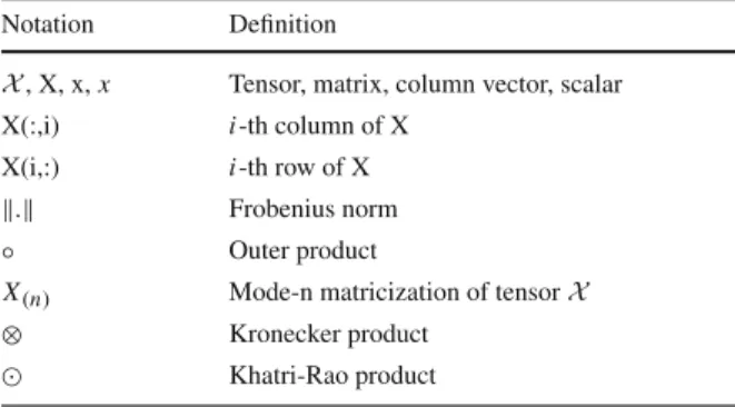
Table 1 Notations
Notation Definition
X, X, x,x Tensor, matrix, column vector, scalar X(:,i) i-th column of X
X(i,:) i-th row of X
. Frobenius norm
◦ Outer product
X(n) Mode-n matricization of tensorX
⊗ Kronecker product
Khatri-Rao product
is formed. Yet, Our method compares each region’s behavior to its normal case. Even the anomaly has little influence on nearby regions, it will be detected once it behaved much different from its normal behavior. In addition, many visual techniques have been proposed to facilitate analyzing spatiotemporal data (Liu et al.2014; Sun et al.
2013,2017a,2017b; Xia et al.2016; Wu et al.2018).
3 Background and preliminaries
Here we list all necessary background knowledge for tensor decomposition and our algorithm frameworkTBAD. Table1provides an overview of the notations we use.
The Kronecker product of two matrices A∈ RI×Jand B, denoted by⊗is defined as Kolda and Bader (2009):
A⊗B= ⎛ ⎜ ⎜ ⎜ ⎝ a11B a12B · · · a1JB a21B a22B · · · a2JB ... ... ... ... aI1B aI2B · · · aI JB ⎞ ⎟ ⎟ ⎟ ⎠
For two matricesA=(a1,a2, . . . ,ak) ,B=(b1,b2, . . . ,bk)with the same num-berkof columns, their Khatri-Rao product, denoted by, is defined as Kolda and Bader (2009):
AB=(a1⊗b1,a2⊗b2, . . . ,ak⊗bk)
3.1 Tensor
A tensor, denoted byX, is a multi-dimensional array, which is an extensional concept of matrix. In general, a N-way tensor(or Nth-order tensor) is a tensor of N dimensions. In particular, a zero-way tensor is a scalar, a one-way tensor is a vector and two-way tensor is a matrix. A N-two-way tensorX ∈ R+I1×I2×···×IN has N ways with the
dimensionality ofI1,I2, . . . ,IN.R+means all the elements ofX are non-negative, which are commonly used in real-world applications.
3.2 Tensor decomposition
Given a tensorX, the CP decomposition (or PARAFAC decomposition) factorizes the tensor into a sum of rank-one tensors (Kolda and Bader2009). For example, given a three-way tensorX ∈RI×J×K, it can be written as Kolda and Bader (2009):
X ≈
R
r=1
ar ◦br◦cr = [[A,B,C]] (1) where R is a positive number andar ∈ RI,br ∈ RJ,cr ∈ RK for r = 1, 2,…, R. PARAFAC decomposition is usually represented in its matrix form[[A,B,C]](Kolda and Bader2009), where the columns of matrixA,B,Care thear,br,cr vectors. In particular, A=(a1,a2, . . . ,aR) ,B=(b1,b2, . . . ,bR) ,C=(c1,c2, . . . ,cR).
As the symbol ’◦’ represents outer product of vectors, each element of the tensor
X can be also written as:
Xi j k ≈ R
r=1
AirBjrCkr
In this work, we use the non-negative CP decomposition in our framework, since it admits a very intuitive interpretation of its latent factors, and non-negativity is inherent to the data being considered.
3.3 Local outlier factor
The local outlier factor (LOF) is a classic anomaly detecting algorithm (Breunig et al.
2000). It detects anomalous data points by comparing each point’s density with its k-nearest neighbors. LOF algorithm assigns scores of being an outlier to each data point. The score is called the local outlier factor(LOF) of a data point. Data points with high LOF value have less local densities than their k-nearest neighbors and are of great probability to represent outliers. A LOF-value around 1 implies that the point’s density is similar to its neighbors, which is of great probability to declare that it is not an outlier. A LOF-value below 1 implies the point has lower density than its neighbors, which also indicates it is not an outlier.
However, it is not time-evolving and may face computational difficulties when dimensionality increases. Thus, we preprocess the data points before using LOF algo-rithm, which is illustrated in Sect.4and the result shows a significant improvement over pure LOF algorithm, which is discussed in Sect.5.
4 TBAD: a tensor-based spatiotemporal anomaly detection method
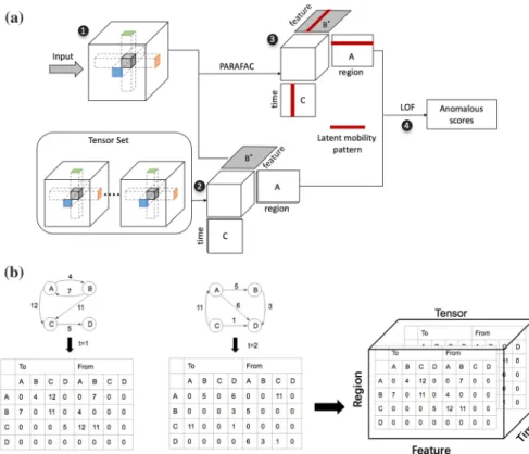
We illustrate the pipeline of our algorithm model in Fig.1a. The procedure consists of four steps. First, we formulate a set of region-feature matrices in consecutive time slices and build up a region-feature-time tensor. Second, we apply non-negative CP
Fig. 1 System description.aPipeline,btensor formulation
decomposition on the tensor and extract latent mobility patterns from factor matrix
B∗. Third, we decompose each upcoming tensor with respect to the former latent patterns(B∗) and capture their dynamic distribution on temporal and spatial dimension. Finally, we compare each region’s co-occurrence of latent patterns with its historical distribution. Anomalous regions often hold a different distribution of latent patterns and we can use the LOF algorithm to find them. Here we assume that anomalous regions are those with different traffic patterns compared to their normal historical situation. In addition, we can also use other classic anomaly detection algorithms such as one-class SVM (Chen et al.2001) rather than LOF to detect anomaly.
4.1 Model formulation
As we discussed above, a tensor can store multi-dimensional information. Thus, we use a tensor to represent traffic flow in a period of time. Suppose that there are K
features to measure a region and a time interval divided intoM smaller time slices, we can construct a tensorX ∈ RN×K×M to indicate a spatiotemporal information, which represents the feature variances of different regions over time. In particular, the elementXi j k denotes the value of j-th feature in i-th region during the period of k-th time slice. Note that there are two notions in time dimension. First, the tensor is built
over a period of time(e.g., a day, a week or a year). The time interval is further divided into several fixed time slices, of which the granularity is determined according to the length of the time interval. For example, the length of the time slices can be set to one hour when the interval is a day, or a day when the interval is a week. In our experiment, the interval is a day and the length of time slices is 2-h.
The features used in the tensor are selected according to different data sources. The following describes the situation of tensor formulation using yellow taxi data in NYC. Suppose that the number of region is N, which is pre-determined. Then we use 2Nfeatures to measure the incoming and outgoing flow of a certain region. The first N features indicate the number of taxi trips leaving region-i. And the nextN
features indicate the number of trips entering region-i. To be specific, for region-i,
X[i,j,k]denotes the number of trips from region-ito region-jink-th time slice and
X[i,N+j,k]denotes the number of trips from region-jto region-iink-th time slice, respectively. In particular, bothX[i,i,k],X[i,N+i,k]denotes the number of trips traveling inside region-i (one of which is omitted in analysis to avoid redundancy). Figure1b shows an numerical example of our proposed tensor formulation method.
4.2 Extracting basic mobility patterns
With the large volume of historical traffic data, our goal is to find several basic mobility patterns which can be used to represent normal traffic behavior. In other words, a region’s traffic pattern can be interpreted as linear combination of the former basic patterns. In this case, we can interpret a region’s traffic patterns with the interpretation of the basic patterns. Technically, we are going to produce a factor matrixB∗to extract basic mobility patterns in a city. We first get all the tensorsXi(i = 1,…,n) to be trained andB∗is calculated by:
B∗= ar gmi n Ai,Ci,B∗≥0 n i=1 (Xi−[[Ai,B∗,Ci]]2+αAi−Ai−12+βCi−Ci−12) (2)
B∗is the feature-component (basic mobility pattern) factor matrix. We supposeB∗to be the common factor matrix of all the training tensors. Therefore, it stores the most common relationship between feature and basic traffic patterns and Ai,Ci matrices capture the dynamic spatial and temporal distribution of basic patterns. Thus,B∗can represent the most general basic mobility patterns on the training set.
The coefficientsα, βhere are used to control smoothness on factor matricesAiand
Ci, which aims to eliminate the anomaly in the training set. Since the training set is not labelled, we suppose that imposing smoothness can eliminate the influence of the anomalies on the extracted latent patterns. The values of the two coefficients are set according to the specific situations.
It is easy to illustrate how this can be used in online situation. When the latest tensor
Xn+1arrives, we can solve the optimization problem (2) by applyingXn+1to gain a newB∗. As time evolves, we can replace the oldest tensorX1with the latest tensor
Besides, when dealing with time dependent models, different time intervals are not treated equally. In general, latest ones are more important than the ones in the past. To achieve this goal, additional coefficients can be added to the objective function.
B∗= ar gmi n Ai,Ci,B∗≥0 n i=1 γiXi − [[Ai,B∗,Ci]]2 (3)
γicontrols the importance ofith-time interval. For simplicity, the experiments in our work still use (2) as objective function.
4.3 Factorizing upcoming tensor
With the factor matrixB∗we got in Sect.4.2, we apply non-negative CP decomposition to the upcoming tensorX, which contains the latest traffic data to be detected, with the constraint that the B (feature-component) factor matrix is equal toB∗:
A,C =ar gmi n
A,C≥0
X− [[A,B∗,C]] (4)
This is calculated under the assumption that the basic traffic patterns do not change dramatically in a short time. Thus we can use the same subspace to capture the relation-ship between feature and latent traffic patterns. With the same relationrelation-ship between feature and latent patterns, we can then use the factor matrix A andC to capture the patterns’ distribution on spatial and temporal dimension. In particular, matrix A
(region-component matrix) describes the patterns’ co-occurrence on a certain region. For example, A[i,k]captures thek-th pattern’s occurrence oni-th region. The larger the value is, the more likely that region-i behaves in tune with pattern-k. MatrixC
(time-component matrix) describes the pattern’s temporal activity level. For example,
C[j,k]indicates the activity level ofk-th pattern in j-th time slice. The larger the value is, the more traffic flow behaves in accord with pattern-kin j-th time slice.
4.4 Detecting anomaly by factor matrices
According to Sects. 4.2and4.3, we got factor matrices Ai(i = 1, . . . ,n)for the training tensors and factor matrixAfor the detecting tensor. In particular, the row vector
Ai(k,:)in each factor matrix Ai represents the patterns’ historical co-occurrence on region-k. As discussed previously in the beginning of Sect.4, we hold the assumption that anomalous regions are those behave differently from their historical behavior. Thus we apply LOF algorithm to Ai(k,:)(i = 1,…,n) and A(k,:)to detect whether the co-occurrence of the basic patterns onk-th region has changed and the lof-value is denoted aslo fk. Moreover,lo fkwill be a large value if the region shows such different traffic behavior that the co-occurrence of basic patterns changed dramatically. Thus we found regions’ extent of anomaly by their lof-value.
4.5 Update rule
We solve the above optimization problem (2) using block coordinate descent (Kim et al.2014) and a multiplicative rule based on a tensor time series of the historical data. We treat B,At,Ct(t = 1, . . . ,n) as 2n+1 blocks and the update order is
A1→C1→ A2→C2→ · · ·An→Cn→ B∗. In particular, the update rules are: 1. solve A(t),t =1,2, . . . ,n A(t)=ar gmi n A≥0 (|| XTt,(1)−(CtB)AT||2+α||AT −ATt−1||2) =ar gmi n A≥0 || X−F AT||2 her e X = X T t,(1) √α ATt−1 ,F= C√tαB I Aj k ← Aj k ( XTF)j k (AFTF) j k 2. solve C(t),t =1,2, . . . ,n C(t)=ar gmi n C≥0 (|| XtT,(3)−(BAt)CT||2+β||CT −CtT−1||2) =ar gmi n C≥0 || X−FCT||2 her e X= X T t,(3) √ βCtT−1 ,F= B√βAt I Cj k ←Cj k ( XTF)j k (C FTF) j k 3. solve B∗ B∗=ar gmi n B≥0 n t=1 ||XTt,(2)−(CtAt)BT||2 =ar gmi n B≥0 || X−F BT||2 her e X= ⎛ ⎜ ⎜ ⎜ ⎜ ⎝ X1T,(2) X2T,(2) ... XTn,(2) ⎞ ⎟ ⎟ ⎟ ⎟ ⎠,F= ⎛ ⎜ ⎜ ⎜ ⎝ C1A1 C2A2 ... CnAn ⎞ ⎟ ⎟ ⎟ ⎠ Bj k← Bj k ( XTF) j k (B FTF) j k
where I is the Identity matrix. The Xt,(n) denotes the n-mode matricized version (Cichocki et al.2009) of Xt.
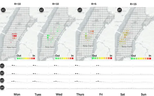
Fig. 2 Interpretation of latent patterns; (a1, a2, a3, a4) shows the spatial information of patters on the map and (b1, b2, b3, b4) reveals the pattern’s temporal distribution respectively
5 Empirical evaluation
We appliedTBADto real-world data sets in order to verify its accuracy. The experiment was conducted on New York City yellow taxi trip data in 2014.1It contained around 3,000,000 yellow cab trip data at New York City in 2014, which included trips’ origin, destination, pick-up time, drop-off time and passenger count. We first used TBAD
to find the anomaly region based on the traffic data. We used R = 5,10,15 in our experiments and how to choose R are discussed in the next section. Special event corresponding to the anomaly region should be found to verify the correctness of
TBAD. Then we compared the error rate ofTBADwith similar approach with untrained model and pure LOF.
5.1 Interpretation of basic mobility patterns
To illustrate how we interpret the extracted patterns, we visually summarize the spa-tial and temporal information by applying basic visual representations on the map of Manhattan. As shown in Fig.2a1–a4, we place a grid on the top of the map to demonstrate the division of regions. The flow pattern of each region is encoded with a node inside the grid, with the size of node representing the volume of the flow, and the color representing the direction of the flow. A red-to-yellow-to-green color gradient is adopted here to indicate the average flow direction, with the red color indicating that the region contains more incoming trips and the green indicating more 1 https://data.cityofnewyork.us/view/gn7m-em8n.
the outgoing trips. We further demonstrate the temporal distribution of the specific pattern (a1–a4) in Fig. 2b1–b4. As the length of time slices is 2-hour, we plot the temporal distribution of these patterns in each time slice. The size of nodes encodes the activity level so as to highlight time slices in which the pattern is more significant. Specifically, the size is set according to theCi(i =1, ...,n)factor matrices we got in Sect.4.2. For example, the activity level ofkth-pattern in jth-time slices inith-time interval isCi[j,k]. Figure2a1, a2 illustrate two distinct patterns when set R = 10, and Fig.2b1, b2 reveal their corresponding temporal characteristics. These patterns mainly appear around the center of Manhattan in 6 and 10 a.m. of the weekdays and disappear in weekends. This could reveal the morning peak of these regions, dur-ing which people flood into Manhattan Midtown (e.g., Rockefeller Center) to go to work.
To reveal the impact of parameter R on the extracted patterns, we decrease and increase the value of R to 5 and 15 as shown in Fig. 2a3, a4 respectively. When the value of R is small, the extracted patterns are mostly aggregated, resulting in a mixture of incoming and outgoing flows, which makes it diffi-cult to observe separately. On the contrary, if R is too large, some extracted patterns will be less meaningful. For example, Fig. 2b4 shows one of the tem-poral patterns when R is set to 15, which is inactive all the time, providing no useful information and should be considered as noise. Generally, patterns are more interpretative when the number of latent patterns increases. However, it will also produce more noise and less meaningful information. Thus, a prop-erly chosen R should provide us with more meaningful and less noisy pat-terns.
5.2 Case study
In order to locate the anomalous region easily, we divided the New York City into mesh-grid according to the longitude and the latitude. Then we computed anomaly score for each region. Regions with high anomaly scores were the anomalies we were trying to find. Following are several cases thatTBADgenerate from the third-season data in 2014:
Electric Zoo Music Festival at Randall’s Island Park Figure3 shows the anomaly region detected byTBAD on August 30 and 31. In Fig.3, we have calculated the anomaly-score of the highlighted region on every Saturday. Most of the score was around 1, while the score on August 30th was 11.26. That value was significantly higher than the average score. So we considered August 30th as an anomalous date for that region. According to the speculation, we found that Electric Zoo music festival was held at Randall’s Island park during that period.
Queen Mary 2(Ocean Liner) New York Arrival Figure4shows the extraordinary taxi flow between two regions shown on the map on September 27. The score(Day index 25) of those regions on September 27th was around 18.66, which was clearly an outlier in the diagram. Actually, ocean cruiser Queen Mary 2 arrived at New York Manhattan
Fig. 3 Anomalous region and anomaly score diagram on August 30
Fig. 4 Anomalous region and anomaly score diagram on September 27
Cruiser Terminal on that day, while she used to dock at New York Brooklyn Cruiser Terminal, which is located at the red area. Thus, we thought that the unusual docking terminal forced many people to travel from Brooklyn to Manhattan.
U.S. OPEN (Tennis Tournament) Semifinal and Final We observed a high anomaly score on September 6 and 7 in the region surrounding Flushing Meadows-Corona Park as shown in Fig.5. For all Sundays and Saturdays in the third season of 2014, we can clearly find the anomaly which is around September 6 through the diagram with an anomaly score of 12.22.
After checking U.S. OPEN’s schedule, we found out that men’s singles semifinals was on September 6 and women’s singles final was on September 7. These matches involved famous tennis players such as Novak Djokovic, Roger Federer and Serena Williams. That would be reason why people were gathering there at a certain time. Except for the tournament, there existed another anomaly point with a score of 5.65 in the following week. This anomalous point indicated another special event in the park, which was the World Maker Faire on September 20 according to our search result.
Fig. 5 Anomalous region and anomaly score diagram on September 6 and 7
Fig. 6 Our model successfully detect the Music Festival (Left) and the U.S.OPEN (Right). And the untrained model cannot detect them and shows much more irregular results
5.3 Compared with untrained model
We have compared our TBAD framework with existing approach using untrained model. As untrained models share no similarity in factor matrices, the latent mobility patterns extracted from the tensor may differ a lot. Thus, the feature vectors extracted from the factor matrixAhave no baseline meaning and cannot be compared altogether. We have done experiments and the result in Fig.6shows that untrained model may produce massive wrong detection results.
5.4 Compared with LOF
We have also compared our method with the existing approach using LOF. Since LOF algorithm detects anomaly in numerous points and a point can only denote one time slice, time dimension is not considered, resulting in the insensitivity to the change in a dynamic traffic system.
We have done some comparison to demonstrate the idea. The result is shown in Fig.3. The red and yellow points correspond to the result of our model and LOF
respectively. The figure shows that our method is much more sensitive and effective than directly using LOF algorithm. Although the LOF results still have two days sharing the highest score, it is quite similar to other points and thus difficult for us to distinguish.
6 Conclusion
In this paper, we present a novel framework for detecting anomalous event. It integrates tensor decomposition and LOF algorithm to localize anomaly in a given time interval. We demonstrate the power ofTBADthrough its application in New York City yellow taxi data. We have done a case study based on anomalous event found by our system and several comparison with other present techniques. In the future, we would apply the framework to more areas such as pollution monitoring and severe weather warning. Furthermore, we would design a multi-functional visualization system to make the anomaly visually shown to the users and let the users to interact with the system to further improve its accuracy.
References
Bahadori MT, Yu QR, Liu Y (2014) Fast multivariate spatio-temporal analysis via low rank tensor learning. In: Advances in neural information processing systems, pp 3491–3499
Bai Y, Tezcan J, Cheng Q, Cheng J (2013) A multiway model for predicting earthquake ground motion. In: ACIS international conference on software engineering, artificial intelligence, networking and parallel/distributed computing (SNPD), pp 219–224
Breunig MM, Kriegel HP, Ng RT, Sander J (2000) Lof: identifying density-based local outliers. ACM Sigmod Rec 29:93–104
Chandola V, Banerjee A, Kumar V (2009) Anomaly detection: a survey. ACM Comput Surv (CSUR) 41(3):15
Chen Y, Zhou XS, Huang TS (2001) One-class svm for learning in image retrieval. IEEE Image Process 1:34–37
Cichocki A, Zdunek R, Phan AH, Amari SI (2009) Nonnegative matrix and tensor factorizations: applica-tions to exploratory multi-way data analysis and blind source separation. Wiley, New York Fanaee-T H, Gama J (2015) Eigenevent: an algorithm for event detection from complex data streams in
syndromic surveillance. Intell Data Anal 19(3):597–616
Fanaee-T H, Gama J (2016a) Tensor-based anomaly detection: an interdisciplinary survey. Knowl Based Syst 98:130–147
Fanaee-T H, Gama J (2016b) Event detection from traffic tensors: a hybrid model. Neurocomputing 203:22– 33
Fanaee-T H, Gama J (2014) An eigenvector-based hotspot detection. arXiv preprintarXiv:1406.3191
Gauvin L, Panisson A, Cattuto C (2014) Detecting the community structure and activity patterns of temporal networks: a non-negative tensor factorization approach. PloS ONE 9(1):e86028
Jiang M, Cui P, Faloutsos C (2016) Suspicious behavior detection: current trends and future directions. IEEE Intell Syst 31(1):31–39
Kim J, He Y, Park H (2014) Algorithms for nonnegative matrix and tensor factorizations: a unified view based on block coordinate descent framework. J Global Optim 58(2):285–319
Kolda TG, Bader BW (2009) Tensor decompositions and applications. SIAM Rev 51(3):455–500 Kotsia I, Guo W, Patras I (2012) Higher rank support tensor machines for visual recognition. Pattern Recogn
45(12):4192–4203
Liu S, Cui W, Wu Y, Liu M (2014) A survey on information visualization: recent advances and challenges. Visual Comput 30(12):1373–1393
Liu D, Weng D, Li Y, Bao J, Zheng Y, Qu H, Wu Y (2017) SmartAdP: Visual analytics of large-scale taxi trajectories for selecting billboard locations. IEEE Trans. Vis. Comput. Graphics 23(1):1–10 Liu Y, Zhou B, Chen F, Cheung DW (2016) Graph topic scan statistic for spatial event detection. In:
Pro-ceedings of the 25th ACM International on Conference on Information and Knowledge Management. ACM, pp 489–498
Mao HH, Wu CJ, Papalexakis EE, Faloutsos C, Lee KC, Kao TC (2014) Malspot: Multi2 malicious network behavior patterns analysis. In: Pacific-Asia conference on knowledge discovery and data mining. Springer, pp 1–14
Matsubara Y, Sakurai Y, Faloutsos C, Iwata T, Yoshikawa M (2012) Fast mining and forecasting of complex time-stamped events. In: Proceedings of the ACM SIGKDD international conference on Knowledge discovery and data mining, pp 271–279
Nomikos P, MacGregor JF (1994) Monitoring batch processes using multiway principal component analysis. AIChE J 40(8):1361–1375
Papalexakis EE, Faloutsos C, Sidiropoulos ND (2012) Parcube: sparse parallelizable tensor decompositions. In: Joint European conference on machine learning and knowledge discovery in databases. Springer, pp 521–536
Papalexakis E, Pelechrinis K, Faloutsos C (2014) Spotting misbehaviors in location-based social networks using tensors. In: Proceedings of the international conference on world wide web. ACM, pp 551–552 Paschalidis IC, Smaragdakis G (2009) Spatio-temporal network anomaly detection by assessing deviations
of empirical measures. IEEE/ACM Trans Netw (TON) 17(3):685–697
Prada MA, Dominguez M, Barrientos P, Garcia S (2012a) Dimensionality reduction for damage detection in engineering structures. Int J Mod Phys B 26(25):1246004
Prada MA, Toivola J, Kullaa J, HollméN J (2012b) Three-way analysis of structural health monitoring data. Neurocomputing 80:119–128
Rendle S (2012) Factorization machines with libfm. ACM Trans Intell Syst Technol (TIST) 3(3):57 Rozenshtein P, Anagnostopoulos A, Gionis A, Tatti N (2014) Event detection in activity networks. In:
Proceedings of the 20th ACM SIGKDD international conference on Knowledge discovery and data mining. ACM, pp 1176–1185
Shi L, Gangopadhyay A, Janeja VP (2015) Stensr: spatio-temporal tensor streams for anomaly detection and pattern discovery. Knowl Inf Syst 43(2):333
Sun GD, Liang R, Qu H, Wu Y (2017a) Embedding spatiotemporal information into maps by route-zooming. IEEE Trans. Vis. Comput. Graphics 23(5):1506–1519
Sun G, Tang T, Peng TQ, Liang R, Wu Y (2017b) Socialwave: visual analysis of spatio-temporal diffusion of information on social media. ACM Trans Intell Syst Technol 9(2):15
Sun J, Tao D, Papadimitriou S, Yu PS, Faloutsos C (2008) Incremental tensor analysis: Theory and appli-cations. ACM Trans Knowl Discov Data (TKDD) 2(3):11
Sun J, Tao D, Faloutsos C (2006) Beyond streams and graphs: dynamic tensor analysis. In: Proceedings of the 12th ACM SIGKDD international conference on Knowledge discovery and data mining. ACM, pp 374–383
Sun G, Wu YC, Liang RH, Liu SX (2013) A survey of visual analytics techniques and applications: state-of-the-art research and future challenges. J Comput Sci Tech 28(5):852–867
Tao D, Li X, Hu W, Maybank S, Wu X (2005) Supervised tensor learning. In: IEEE international conference on data mining
Thai-Nghe N, Horváth T, Schmidt-Thieme L (2010) Factorization models for forecasting student perfor-mance. In: Educational Data Mining 2011
Tian X, Zhang X, Deng X, Chen S (2009) Multiway kernel independent component analysis based on feature samples for batch process monitoring. Neurocomputing 72(7):1584–1596
Tork HF, Oliveira M, Gama J, Malinowski S, Morla R (2012) Event and anomaly detection using tucker3 decomposition. In: Workshop on ubiquitous data mining, p 8
Wang XR, Lizier JT, Obst O, Prokopenko M, Wang P (2008) Spatiotemporal anomaly detection in gas monitoring sensor networks. In: Wireless sensor networks: 5th European conference, EWSN 2008. Springer, pp 90–105
Wang J, Gao F, Cui P, Li C, Xiong Z (2014) Discovering urban spatio-temporal structure from time-evolving traffic networks. In: Asia-Pacific web conference. Springer, pp 93–104
Weng D, Zhu H, Bao J, Zheng Y, Wu Y (2018) Homefinder revisited: finding ideal homes with reachability centric multi-criteria decision making. In Proceedings of ACM CHI
Wu Y, Lan J, Shu X, Ji C, Zhao K, Wang J, Zhang H (2018) ITTVIS: Interactive visualization of table tennis data. IEEE Trans Visualization and Comp Graphics 24(1):709–718
Xia J, Chen W, Hou Y, Hu W, Huang X, Ebertk DS (2016) DimScanner: A relation-based visual exploration approach towards data dimension inspection. In: IEEE conference on visual analytics science and technology (VAST). pp 81–90
Xie C, Chen W, Huang X, Hu Y, Barlowe S, Yang J (2014) VAET: A visual analytics approach for e-transactions time-series. IEEE Trans. Vis. Comput. Graphics 20(12):1743–1752
Xu P, Mei H, Ren L, Chen W (2017) ViDX: Visual diagnostics of assembly line performance in smart factories. IEEE Trans. Vis. Comput. Graphics 23(1):291–300
Young WC, Blumenstock JE, Fox EB, McCormick TH (2014) Detecting and classifying anomalous behavior in spatiotemporal network data. In: Proceedings of KDD workshop on learning about emergencies from social information (KDD-LESI 2014), pp 29–33
Yuan J, Zheng Y, Xie X (2012) Discovering regions of different functions in a city using human mobility and pois. In: Proceedings of the ACM SIGKDD international conference on Knowledge discovery and data mining, pp 186–194
Zhang T, Wang X, Li Z, Guo F, Ma Y, Chen W (2017) A survey of network anomaly visualization. Sc China Infor Sci 60(12):121101
Zhao Z, Cheng Z, Hong L, Chi EH (2015) Improving user topic interest profiles by behavior factorization. In: Proceedings of the international conference on world wide web. ACM, pp 1406–1416
Zheng Y, Liu T, Wang Y, Zhu Y, Liu Y, Chang E (2014) Diagnosing New York city’s noises with ubiq-uitous data. In: Proceedings of the ACM international joint conference on pervasive and ubiqubiq-uitous computing, pp 715–725