New Nonlinear Machine Learning Algorithms with
Applications to Biomedical Data Science
by
Xiaoqian Wang
BS, Zhejiang University, 2013
Submitted to the Graduate Faculty of
the Swanson School of Engineering in partial fulfillment
of the requirements for the degree of
Doctor of Philosophy
University of Pittsburgh
2019
UNIVERSITY OF PITTSBURGH
SWANSON SCHOOL OF ENGINEERING
This dissertation was presented
by
Xiaoqian Wang
It was defended on
May 31, 2019
and approved by
Heng Huang, PhD, John A. Jurenko Endowed Professor, Department of Electrical and Computer
Engineering
Zhi-Hong Mao, PhD, Professor, Department of Electrical and Computer Engineering
Wei Gao, PhD, Associate Professor, Department of Electrical and Computer Engineering
Jingtong Hu, PhD, Assistant Professor, Department of Electrical and Computer Engineering
Jian Ma, PhD, Associate Professor, Computational Biology Department, Carnegie Mellon
University
Dissertation Director: Heng Huang, PhD, John A. Jurenko Endowed Professor, Department of
Copyright cby Xiaoqian Wang 2019
New Nonlinear Machine Learning Algorithms with Applications to Biomedical Data Science Xiaoqian Wang, PhD
University of Pittsburgh, 2019
Recent advances in machine learning have spawned innovation and prosperity in various fields. In machine learning models, nonlinearity facilitates more flexibility and ability to better fit the data. However, the improved model flexibility is often accompanied by challenges such as overfitting, higher computational complexity, and less interpretability. Thus, it is an important problem of how to design new feasible nonlinear machine learning models to address the above different challenges posed by various data scales, and bringing new discoveries in both theory and applications. In this thesis, we propose several newly designed nonlinear machine learning algorithms, such as additive models and deep learning methods, to address these challenges and validate the new models via the emerging biomedical applications.
First, we introduce new interpretable additive models for regression and classification and ad-dress the overfitting problem of nonlinear models in small and medium scale data. we derive the model convergence rate under mild conditions in the hypothesis space and uncover new potential biomarkers in Alzheimer’s disease study. Second, we propose a deep generative adversarial net-work to analyze the temporal correlation structure in longitudinal data and achieve state-of-the-art performance in Alzheimer’s early diagnosis. Meanwhile, we design a new interpretable neural network model to improve the interpretability of the results of deep learning methods. Further, to tackle the insufficient labeled data in large-scale data analysis, we design a novel semi-supervised deep learning model and validate the performance in the application of gene expression inference.
Table of Contents Preface . . . xii 1.0 Introduction . . . 1 1.1 Background . . . 1 1.2 Contribution . . . 4 1.3 Notation . . . 5 1.4 Proposal Organization . . . 5
2.0 Additive Model for Small/Medium Scale Data . . . 7
2.1 Motivation . . . 7
2.2 Related Work . . . 8
2.3 FNAM for Quantitative Trait Loci Identification . . . 10
2.4 Generalization Ability Analysis . . . 12
2.5 Experimental Results . . . 18
2.5.1 Data Description . . . 18
2.5.2 Experimental Setting . . . 20
2.5.3 Performance Comparison on ADNI Cohort . . . 21
2.5.4 Important SNP Discovery . . . 21
2.5.5 Performance with Varying Hidden Node Number . . . 22
2.5.6 Running Time Analysis . . . 22
3.0 Uncovering Feature Group via Structured Additive Model . . . 29
3.1 Introduction . . . 29
3.2 Group Sparse Additive Machine . . . 31
3.3 Generalization Error Bound . . . 35
3.4 Experimental Results . . . 39
3.4.1 Performance Comparison on Synthetic Data . . . 40
3.4.2 Performance Comparison on Benchmark Data . . . 42
3.4.4 Interpretation of Imaging Biomarker Interaction . . . 43
4.0 Deep Neural Network for Large-Scale Data . . . 46
4.1 Introduction . . . 46
4.2 Related Work . . . 49
4.2.1 Gene Expression Inference . . . 49
4.2.2 Deep Neural Networks . . . 50
4.3 Conditional Generative Adversarial Network . . . 52
4.3.1 Motivations . . . 52
4.3.2 Deep Generative Model . . . 53
4.4 Generative Network for Semi-Supervised Learning . . . 56
4.4.1 Problem Definition . . . 56
4.4.2 Motivation . . . 56
4.4.3 Semi-Supervised GAN Model . . . 58
4.5 Experimental Results . . . 60
4.5.1 Experimental Setup . . . 60
4.5.1.1 Datasets . . . 60
4.5.1.2 Evaluation Criterion . . . 61
4.5.1.3 Baseline Methods . . . 61
4.5.1.4 Implementation Details of GGAN . . . 62
4.5.1.5 Implementation Details of SemiGAN . . . 63
4.5.2 Prediction of GEO Data via GGAN . . . 63
4.5.3 Prediction of GTEx Data via GGAN . . . 66
4.5.4 Visualization of GGAN Network Relevance . . . 67
4.5.5 Comparison on the GEO Data for SemiGAN . . . 68
4.5.6 Comparison on the GTEx Data for SemiGAN . . . 68
4.5.7 Analysis of Landmark Genes in SemiGAN Prediction . . . 69
5.0 Learning Longitudinal Data with Deep Neural Network . . . 77
5.1 Motivation . . . 77
5.2 Temporal Correlation Structure Learning Model . . . 78
5.2.2 Revisit GAN Model . . . 78
5.2.3 Illustration of Our Model . . . 79
5.3 Experimental Results . . . 80
5.3.1 Experimental Setting . . . 80
5.3.2 Data Description . . . 81
5.3.3 MCI Conversion Prediction . . . 82
5.3.4 Visualization of the Imaging markers . . . 82
6.0 Building An Additive Interpretable Deep Neural Network . . . 85
6.1 Motivation . . . 85
6.1.1 Interpretation of a Black-Box Model . . . 86
6.2 Building An Additive Interpretable Deep Neural Network . . . 87
6.3 Experimental Results . . . 90
6.3.1 Experimental Setting . . . 90
6.3.2 MCI Conversion Prediction . . . 91
6.3.3 Visualization of the Imaging markers . . . 93
6.4 Additive Interpretation Methods for Machine Learning Fairness . . . 94
6.4.1 Problem Definition . . . 95
6.5 Approaching Machine Learning Fairness Through Adversarial Network . . . 96
6.6 Experimental Results . . . 101
7.0 Conclusion . . . 106
List of Tables
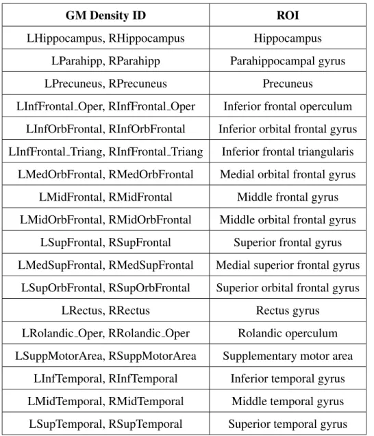
1 36 GM density measures (VBM) matched with disease-related ROIs. . . 24
2 26 volumetric/thickness measures (FreeSurfer) matched with disease-related ROIs. . 25
3 Performance evaluation of FNAM on FreeSurfer and VBM prediction. . . 27
4 Properties of different additive models. . . 31
5 Classification evaluation of GroupSAM on the synthetic data. The upper half use 24 features groups, while the lower half corresponds to 300 feature groups. . . 41
6 Comparison between the true feature group ID (for data generation) and the selected feature group ID by GroupSAM on the synthetic data. . . 42
7 Classification evaluation of GroupSAM on benchmark data. . . 43
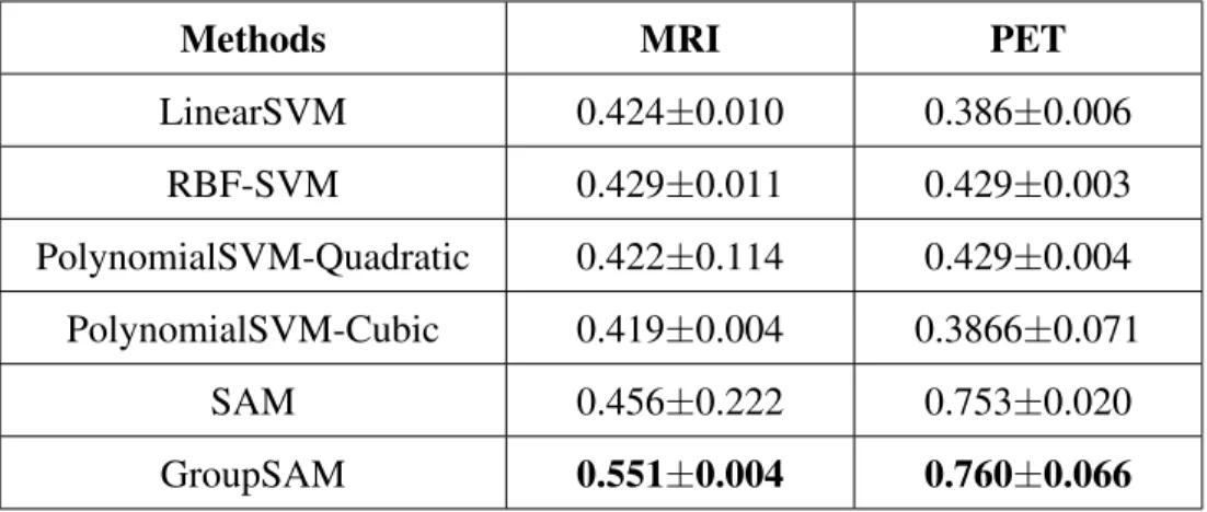
8 Classification evaluation of GroupSAM on MRI and PET data for MCI conversion prediction. . . 44
9 Performance evaluation of GGAN on GEO data. The results of the comparing models are obtained by us running the released codes, except the one marked by (?) on top that is reported from the original paper. . . 64
10 MAE comparison between D-GEX and GGAN modelw.r.t.hidden layer and hidden units numbers for GEO data. . . 64
11 Performance evaluation of GGAN on GTEx data. The results of the comparing models are obtained by us running the released codes, except the one marked by (?) on top that is reported from the original paper. . . 66
12 MAE comparison between D-GEX and GGAN modelw.r.t.hidden layer and hidden units numbers for GTEx data. . . 66
13 MAE comparison on GEO data with different portion of labeled data. . . 73
14 CC comparison on GEO data with different portion of labeled data. . . 73
15 MAE comparison on GTEx data with different portion of labeled data. . . 74
16 CC comparison on GTEx data with different portion of labeled data. . . 74
18 Classification evaluation of ITGAN on MCI conversion prediction with different portion of testing data. . . 92 19 Classification evaluation of ITGAN when involving all 93 ROIs in MCI conversion
List of Figures
1 Performance of RMSE and CorCoe sensitivity of FNAMw.r.t.the number of hidden nodes. . . 19 2 Runtime (in seconds) comparison of FNAMw.r.t. number of hidden nodes. . . 20 3 Heat map (upper) and brain map (below) of the top 10 SNPs identified by FNAM
in VBM analysis. . . 26 4 LocusZoom plot showing Alzheimer’s associated region around rs885561-LIPA
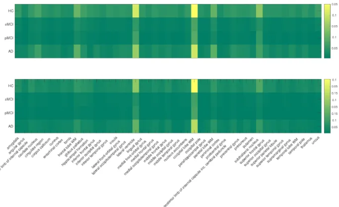
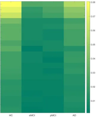
(10M boundary) in Chromosome 10. . . 28 5 Heat maps of the weight matrices learned by GroupSAM on MRI data. The upper
figure shows left hemisphere and the lower shows the right hemisphere. . . 39 6 Cortical maps of the top 10 MRI imaging markers identified by GroupSAM. . . 40 7 Heat maps of the top 20 MRI imaging marker interactions learned by GroupSAM. . 45 8 Illustration of GGAN architecture and its loss functions. . . 52 9 Illustration of the SemiGAN architecture for gene expression inference. . . 57 10 Heatmaps of the importance of landmark genes in the fully connected network of
GGAN model on GEO data. . . 65 11 Illustration of the relevance score of different landmark genes calculated by the
DenseNet architecture in GGAN for GTEx data. . . 72 12 Visualization of the relevance score calculated by SemiGAN for each landmark
gene on GEO data. . . 75 13 Visualization of the relevance score calculated by SemiGAN for each landmark
gene on GTEx data. . . 76 14 Visualization of the feature weights learned from Temporal-GAN. . . 83 15 Illustration of our Temporal-GAN model. . . 84 16 Illustration of the idea of constructing an interpretable additive deep neural network,
17 Illustration of our idea on formulating a deep learning model in an interpretable manner. . . 91 18 Brain map of the top imaging markers identified by ITGAN. . . 93 19 Illustration of the FAIAS model. . . 97 20 Comparison of model performance via classification accuracy and balanced
classi-fication accuracy on three benchmark datasets. . . 101 21 Comparison of prediction fairness via absolute equal opportunity difference,
Preface
The past six years of PhD study has been the best journey I could have in my life. I feel full heart of gratitude as I start writing this thesis. Especially for my doctoral supervisor, Dr. Huang Heng, I sincerely thank him, since I will never have the opportunity to dive into the field of machine learning research without his guidance, trust and strong support. Dr. Huang is a great idol in our lab for being highly self-motivated and confident. We are always deeply impressed by his great passion for research and education. It is Dr. Huang that provided me with a picture of the life of top machine learning researcher, and the main reason to pursue an academic career for my future life. I am really lucky that I can become the student of Dr. Huang and get his guidance along my path toward research and career.
I would also like to thank Dr. Zhi-Hong Mao, Dr. Wei Gao, Dr. Jingtong Hu, and Dr. Jian Ma for being on my PhD committee. I really appreciate the great advice and guidance for the research direction and for academic job hunting. I feel honored to get the inspiring instructions and am grateful to the committee members for their time and help.
Thanks to every member in the CSL lab. Many thanks to Dr. Feiping Nie and Dr. Hong Chen for their guidance and collaboration during my PhD study. Thanks to Kamran, Hongchang, Zhouyuan, Guodong, Feihu, Bin, Lei, Yanfu, Runxue, and Haoteng for the discussion about re-search. I have learned so many things from all members in the CSL lab. I am very lucky that I could be in such a wonderful research group and get the opportunity to make friends and work together with so many great people.
Thanks to my friends, Jia, Akshay, Jie Tang, Xi, Yong, Amy, Jie Xu, Yizhuo, Kun, Zhihui, Yini, Xu, and Mengjiao. Thanks for the company and care. I feel so fortune to be surrounded by good friends who listen to me, understand me, and bring the sunshine in my life. Thanks for making my PhD life colorful and enjoyable and let me feel always supported.
During my job hunting in academia, I have visited over 10 universities and meet with so many great professors. I feel extremely welcomed by the very kind people and am sincerely thankful to Xingbo Wu, Brian Ziebart, Jason Wang, Grace Wang, Xiangnan Kong, Jian Zou, Sudhir Kumar, Zoran Obradovic, Slobodan Vucetic, Haibin Ling, Yuying Xie, Andrew Christlieb, Pang-Ning Tan,
Douglas Schmidt, Stanley Chan, Felix Lin, Saurabh Bagchi, Charles A. Bouman, Milind Kulkarni, Yung-Hsiang Lu, Predrag Radivojac, David Miller, Qun Li, Chao Chen, Steven Skiena, Zhi Ding, and many others. I am grateful to have the opportunity to talk with the professors and learn about how to start the academic career.
Special thanks to my parents, Yong and Qingwei. I could never become who I am without their love and support. Thanks for teaching me to be an upright person and to follow my own enthusiasm and passion. Sincere thanks to my boyfriend, Guohua. Thanks for all the understanding and caring in the past years. He is always my mentor and a great friend. I could never have the courage to take the job at Purdue University without his support. Thanks for always being very patient, caring, and supportive for me during the PhD journey.
1.0 Introduction
1.1 Background
In recent decades, machine learning has achieved unparalleled success in various fields, from automatic translation, object detection to autonomous driving and computer-aided diagnosis. Com-pared with linear methods that hold the assumption of linear association between data, nonlinear models, such as kernels methods, and deep neural network has exhibited a high degree of flexibil-ity and representative power thus has better generalization power in data with complex structures such as images, natural languages, videos and biomedical data.
Despite the wide application and great success, challenges still remain in how to design a good machine learning model. For small to medium scale data, deep learning methods suffer from overfitting problem thus face the problem of bad generalization performance due to training of a model with high variance with limited number of training samples. As for kernel methods, the training involves a large kernel matrix thus introduces high order of computational complexity.
For the training of nonlinear machine learning methods in large-scale data, deep learning mod-els require a large amount of labeled data to build an inference network with satisfying perfor-mance. However, the collection of large libraries of labeled data is still difficult and expensive. In many machine learning applications, it typically requires great effort of human annotators or expensive special devices to label samples. On the contrary, unlabeled data is much easier and less expensive to achieve. To guarantee the quality of the model while reduce the cost of acquiring labels, lots of effort has been made on semi-supervised learning such that the unlabeled data can be better utilized to strengthen the performance of supervised learning. Based on the difference in how to incorporate the information from unlabeled data, semi-supervised classification models can be divided into different types, such as self-training, generative model, co-training, semi-supervised SVM, graph-based methods,etc. See [177, 86] for detailed background on semi-supervised learn-ing models.
Moreover, deep learning models with state-of-the-art performance are usually formulated as black boxes, making it difficult to interpret how the models make decisions. In areas such as health care, autonomous driving and job hiring, human end-users cannot blindly and faithfully trust the predictions from a well-performed model without knowing the mechanism behind the model behavior. The poor interpretability of black-box models can trigger trust issues from human users. It remains an important problem of how to properly address the above challenges when designing new machine learning models for different scale of data in order to improve the trustworthiness and performance of the model.
On the other hand, the rapid development of high-throughput technology has spawned detailed molecular, cellular and pathological features of many diseases, which enables deep and system-atic study in medical research. The availability of comprehensive biological data not only helps researchers around the world to share genomic and clinical information, but also helps to analyze molecular characteristics of serious diseases that threaten human health.
In addition to unprecedented opportunities to uncover vast amounts of biological knowledge, the emergence of large-scale biological data has also brought enormous challenges to processing and interpretation of data. With a large amount of biological data, there is an urgent need for reliable computing models to integrate complex information in an accurate and efficient manner.
For example, Alzheimer’s Disease (AD) is the most common form of dementia, which triggers memory, thinking, and behavior problems. The genetic causal relationship of AD is complex [7] and therefore presents difficulties in the prevention, diagnosis and treatment of this disease. Recent advances in multimodal neuroimaging and high throughput genotyping and sequencing techniques bring an emerging research field, imaging genomics, which provides exciting new opportunities to ultimately improve our understanding of brain disease, their genetic architecture, and their influ-ences on cognition and behavior.
The rapid progress in neuroimaging techniques has provided insights into early detection and tracking of neurological disorders [157]. Later research interest in imaging neuroscience has fo-cused on Genome Wide Association Studies (GWAS) to examine the association between genetic markers, called Single Nucleotide Polymorphisms (SNPs), and imaging phenotypes [154, 27], with the goal of finding explanations for the variability observed in brain structures and functions. However, these research works typically study associations between individual SNPs and
individ-ual phenotypes and overlook interrelated structures among them. To better understand the genetic causal factors of brain imaging abnormalities, previous works have laid great emphasis on identi-fying relevant QTL [144, 118], which related high-throughput SNPs to imaging data and enhanced the progress and prosperity of neuroscience research. Besides, extensive work has been proposed to predict MCI conversion using neuroimaging data [123, 55]. Previous methods usually for-mulate MCI conversion prediction as a binary classification (distinguishing MCI converters from non-converters) [123, 156] or multi-class classification problem (when considering other classes such as AD or health control (HC)) [55, 150], where the methods take the neuroimaging data at baseline time as the input and classify if the MCI samples will convert to AD in years.
The development of efficient and effective computational models can greatly improve under-standing of complex human diseases. For example, a regression model can be used to reveal the association between different disease data type. Clustering models reveals the relationship between different patients, thereby promoting the development of individualized personalized medicine.
To facilitate the prosperity in Alzheimer’s study, ADNI collects abundant neuroimaing, genetic and cognitive tests data for the study of this disease. Another focus of this thesis is to propose appropriate models to learn the association between different types of data such that the genetic basis as well as biological mechanisms of brain structure and function can be extracted. In addition, since AD is a progressive neurodegenerative disorder, we propose to look into the information conveyed in the longitudinal data. Specifically, it is inspiring to study the prodromal stage of Alzheimer’s, MCI, which exhibits a good chance of converting to AD. In all the above studies, we propose to automatically find predominant genetic features/regions of interests (ROIs) which are responsible for the development of AD. Such studies can provide reference for disease diagnosis and drug design.
The goal of this thesis is to put forward novel computational models to address the challenges in designing new machine learning models for different scales of data, and utilize these new models to enhance the understanding in the genesis and progression of severe diseases like Alzheimer’s disease.
1.2 Contribution
We summarize our contribution as follows:
• We propose a novel efficient additive model (FNAM) to address the overfitting problem of nonlinear machine learning in small to medium scale data. We provide rigorous theoretical generalization error analysis on our model. In particular, different from conventional analysis with independent samples, our error bound is under m-dependent observations, which is a more general assumption and more appropriate for the high-throughput complex genotypes and phenotypes.
• A new group sparse nonlinear classification algorithm (GroupSAM) is proposed by extend-ing the previous additive regression models to the classification settextend-ing, which contains the LPSVM with additive kernel as its special setting. To the best of our knowledge, this is the first algorithmic exploration of additive classification models with group sparsity.
• Theoretical analysis and empirical evaluations on generalization ability are presented to sup-port the effectiveness of GroupSAM. Based on constructive analysis on the hypothesis error, we get the estimate on the excess generalization error, which shows that our GroupSAM model can achieve the fast convergence rate O(n−1) under mild conditions. Experimental results demonstrate the competitive performance of GroupSAM over the related methods on both simulated and real data.
• We propose a novel semi-supervised regression framework based on generative adversarial network (GAN) to address the lack of labeled data in large-scale machine learning problem. A new strategy is introduced to stabilize the training of GAN model with high-dimensional output.
• We propose the first longitudinal deep learning model for MCI conversion prediction and achieve state-of-the-art performance in Alzheimer’s early detection.
1.3 Notation
Throughout this thesis, unless specified otherwise, upper case letters denote matrices, e.g.,
X, Y. Bold lower case letters denote vectors, e.g.,w, b. Plain lower case letters denote scalars, e.g., a, γ. wi denotes the i-th element of vector w. wi denotes the i-th row of matrixW. wj
orw(j)denotes the j-th column ofW. w
ij denotes the ij-th element of matrix W. kwk2 orkwk denotes the `2-norm of vector w:
r P
i
w2
i. kWkF denotes the Frobenius norm of matrix W:
kWkF = rP i P j w2 ij = r P i
kwik2. kWk1 denotes the `1 norm: kWk1 = P
i
P
j
|wij|. kWk∗ denotes the trace norm (a.k.a.nuclear norm): kWk∗ =P
i
σi, whereσi is thei-th singular value of
W.
Specially, ddenotes the dimension of the feature vector, i.e.,number of SNPs. n denotes the number of patients. crepresents the number of QTs. X = [x1, x2, . . . , xn]T ∈ Rn×d denotes the input SNP matrix, where each row ofX represents the genetic variants of each patient. Y = [y1, y2, . . . , yn]T∈
Rn×crepresents the input imaging feature matrix where each row ofY denotes the phenotype of one patient. I stands for the identity matrix, and 1 stands for a vector with all elements being 1.
1.4 Proposal Organization
The rest of the proposal is organized as follows. In Chapter 2, we introduce a new additive model for addressing the challenges of overfitting and less interpretability in nonlinear machine for small to medium scale data. We propose the model in an efficient manner with the time complexity the same as linear models and also provide theoretical analysis on the convergence properties of the model. In Chapter 3, we answer the question of how to analyze the feature interaction in ad-ditive model with a new adad-ditive classification model. We proved the convergence property of our new model, which has a satisfactory learning rate with polynomial decay. We conduct extensive experiments on synthetic and real data to validate the model performance. In Chapter 4 we propose two new deep learning models for addressing the problem of lacking labeled data in non-linear
ma-chine learning. We propose the two new models on the basis of generative adversarial network and improve the model performance by effectively learning from the labeled data and large amount of unlabeled data. We show extensive results in the application of gene expression inference to validate the performance. In Chapter 5 we design a new generative model to analyze the longitu-dinal structure in the data and achieve state-of-the-art performance in MCI conversion prediction. Next in Chapter 6 we propose a new idea to build self-explaining deep neural network via additive model and validate the performance in MCI conversion prediction. Finally, we conclude the thesis in Chapter 7 and propose some open problems and future direction.
2.0 Additive Model for Small/Medium Scale Data
2.1 Motivation
In previous works, several machine learning models were established to depict the relations between SNPs and brain endophenotypes [148, 162, 176, 151, 59]. In [148, 176, 151, 59], the au-thors used the low-rank learning models or structured sparse learning models to select the imaging features that share common effects in the regression analysis. [162] applied the LASSO regression model to discover the significant SNPs that are associated with brain imaging features. However, previous works use linear models to predict the relations between genetic biomarkers and brain endophenotypes, which may introduce high bias during the learning process. Since the influence of QTL is complex, it is crucial to design appropriate non-linear model to investigate the genetic biomarkers (due to the limited size of biological data, deep learning models don’t work well for our problem). Besides, most previous computational models on genotype and phenotype studies did not provide theoretical analysis on the performance of the models, thus leaves uncertainty in the validity of the models.
To tackle with these challenging problems, in this chapter, we propose a novel and efficient nonlinear model for the identification of QTL. We apply our model to the QTL identification of Alzheimer’s disease (AD), the most common cause of dementia. By means of feedforward neural networks, our model can be flexibly employed to explain the non-linear associations be-tween genetic biomarkers and brain endophenotypes, which is more adaptive for the complicated distribution of the high-throughput biological data. We would like to emphasize the following contributions of our work:
• We propose a novel additive model with generalization error analysis. In particular, dif-ferent from conventional analysis with independent samples, our error bound is under m -dependent observations, which is a more general assumption and more appropriate for the high-throughput complex genotypes and phenotypes.
• Our model is efficient in computation. The time complexity of our model is linear to the number of samples and number of features in the data. Experimentally we showed that it only takes a few minutes to run our model on the ADNI data.
• Experimental results demonstrate that our model not only identifies several well-established AD-associated genetic variants, but also finds out new potential SNPs.
2.2 Related Work
In QTL identification of brain imaging abnormalities, the goal is to learn a prediction function which estimates the imaging feature matrix Y = [y1, y2, . . . , yn]T ∈
Rn×c given the genetic informationX = [x1, x2, . . . , xn]T ∈ Rn×d. Meanwhile, we want to weigh the importance of each SNP in the prediction according to the learning model. The most straightforward method is least square regression, which learns a weight matrix W ∈ Rd×c to study the relations between
SNPs and brain endophenotypes. W is an intuitive reflect of the importance of each SNP for the prediction of each endophenotype.
Based on least square regression, several models were proposed for QTL identification. In [139, 162], the authors employed sparse regression models for the discovery of predominant ge-netic features. In [40, 148], low-rank constraint was imposed to uncover the group structure among SNPs in the association study.
In the identification of QTL, previous works mainly use linear models for the prediction. How-ever, according to previous studies, the biological impact of genetic variations is complex [95] and the genetic influence on brain structure is complicated [108]. Thus, the relations between genetic biomarkers and brain-imaging features may not be necessarily linear and the prediction with linear models is likely to trigger large bias.
To depict the non-linear association between genetic variations and endophenotypes, neural networks introduce a convenient and popular framework. [122] proposed feed forward neural networks with random weights (FNNRW), which can be formed as:
f(x) =
h
X
t=1
wherex = [x1, x2, . . . , xd] ∈ Rd is the input data, his the number of hidden nodes, vt|ht=1 =
[vt1, vt2, . . . , vtd] ∈ Rd is the parameter in the hidden layer for t-th hidden node, bt ∈ R is
the corresponding bias term, hvt,xi = d
P
j=1
vtjxj represents Euclidean inner product, φ(.) is the
activation function, andat∈Ris the weight for thet-th hidden node.
As is analyzed in [60, 112], FNNRW enjoys an obvious advantage in computational efficiency over neural nets with back propagation. In Eq. (2.1), vt and bt are randomly and independently
chosen before hand, and the randomization in parameter largely relieves the computational burden. FNNRW is aimed at estimating only the weight parameter at|
h
t=1thus is extremely efficient. Such property makes FNNRW more appropriate for analysis of the high-throughput data in Alzheimer’s research.
[112] constructed a classifier using FNNRW where they conduct classification on the featurized data as shown in Eq. (2.1). The classification model can be easily extended to the regression scenario with the objective function formulated as:
min at|ht=1 Y − h X t=1 φ(XvTt +bt1)at 2 F +γ h X t=1 katk22 , (2.2)
where γ is the hyper-parameter for the regularization term and at = [a1, a2, . . . , ac] ∈ Rc is
the weight parameter of thet-th hidden node forcdifferent endophenotypes. As discussed above, Problem (2.2) can be adopted to efficiently estimate the nonlinear associations between genetic variations and brain endophenotypes. However, since the parameters of hidden layer is randomly assigned, traditional FNNRW model makes it hard to evaluate the importance of each feature.
To tackle with these problems, we propose a novel additive model in next section, which not only maintains the advantage of computational efficiency of FNNRW but also integrates the flexibility and interpretability of additive models.
2.3 FNAM for Quantitative Trait Loci Identification
We propose new Additive Model via Feedforward Neural networks with random weights (FNAM) as: fa(X) = h X t=1 d X j=1 φ(vtjxj +bt1)at, (2.3)
where we distinguish the contribution of each feature xj and formulate the model in an additive
style for the prediction. Similar to that of FNNRW, we propose to optimize the least square loss between the ground truth endophenotype matrixY and the estimationfa(X)with`2-norm penal-ization, then we propose the following objective function:
min at|ht=1 Y − h X t=1 d X j=1 φ(vtjxj +bt1)at 2 F +γ h X t=1 katk 2 2 , (2.4)
For simplicity, if we defineA = [a1, a2, . . . , ah]T ∈Rh×cas the weight parameter for hidden
nodes, andG∈Rn×h such that
G= d P j=1 φ(v1jx1j+b1) . . . d P j=1 φ(vhjx1j +bh) .. . . . . ... d P j=1 φ(v1jxnj+b1) . . . d P j=1 φ(vhjxnj+bh) , (2.5)
then we could rewrite our objective function Problem (2.4) as:
min A kY −GAk 2 F +γkAk 2 F . (2.6)
Take derivative w.r.t. Ain Problem (2.6) and set it to 0, we get the closed form solution of A
as below:
A= (GTG+γI)−1GTY . (2.7) As discussed in the previous section, one obvious advantage of FNAM over FNNRW is that FNAM considers the role of each feature independently in the prediction, thus makes it possible to interpret the importance of each SNP in the identification QTL, which is a fundamental goal of jointly studying genetic and brain imaging features.
Algorithm 1Optimization Algorithm of FNAM for QTL Identification. Input:
SNP matrixX ∈Rn×d, endophenotypeY ∈
Rn×c, number of hidden nodesh, parameterγ. Output:
Weight matrixA ∈Rh×cfor the hidden nodes. Weight matrixW ∈
Rd×cshowing the relative importance of thedSNPs in the prediction.
1: Initializethe weight matrixV ∈Rh×drandomly according to uniform distributionU(0, 1).
2: Initializethe bias termb∈Rh randomly according to uniform distributionU(0, 1).
3: 1. ComputeGmatrix according to the definition in Eq. (2.5).
4: 2. UpdateAaccording to the solution in Eq. (2.7)
5: 3. ComputeW according to the definition in Eq. (2.9).
Here we discuss how to estimate the role of each feature in FNAM. To separate the contribution of each feature, we rewrite Eq. (2.3) as below:
fa(X) = d X j=1 ( h X t=1 φ(vtjxj+bt1)at), (2.8)
which indicates that the prediction functionfa(X)can be regarded as the summation ofd terms,
where thej-th term
h
P
t=1
φ(vtjxj +bt1)atdenotes the contribution of thej-th feature.
Naturally, if we normalize the magnitude of the j-th term with the `2-norm of xj, we could
get a good estimation of the significance of thej-th feature. As a consequence, we could define a weight matrixW ∈Rd×cto show the importance of thedSNPs in the prediction of thecimaging
features respectively, such that:
wjl= h P t=1 φ(vtjxj +bt1)atl kxjk , j = 1, . . . d, l= 1, . . . c , (2.9)
We summarize the optimization step of AFNNRW in Algorithm 1 and provide rigorous con-vergence proof of AFNNRW in the Appendix.
Time Complexity Analysis: We summarize the optimization steps of FNAM in Algorithm 1. In Algorithm 1, the time complexity of Step 1 (computingG) isO(ndh), the time complexity of Step 2 (computingA) is O(h2n+hnc), and the time complexity of Step 3 (computing W) is
O(ndhc), wheren is the number of patients,ddenotes the number of SNPs, and crepresents the number of brain endophenotypes. Typically, we haved > handd > cin the identification of QTL, thus the total time complexity of Algorithm 1 isO(ndhc).
2.4 Generalization Ability Analysis
In this section, based on the real situation of biological data, we provide theoretical analysis on the approximation ability of our FNAM model and derive the upper bound of generalization error. In most previous works, theoretical analysis is based on the hypothesis of independent and identically distributed (i.i.d.) samples. However, the i.i.d. sampling is a very restrictive concept that occurs only in the ideal case. As we know, the acquisition of high-throughput biological data involves complicated equipments, reagents as well as precise operation of highly trained techni-cians, which usually introduce variations to the data during the measurement process [77]. Thus, the i.i.d. sampling assumption is not appropriate for the high-throughput biological data analysis. In this section, we provide a learning rate estimate of our model in a much general setting, i.e.,
m-dependent observations [96].
For simplicity, here we consider the prediction of only one brain endophenotypey∈Rn, which
could be easily extended to the case with multiple endophenotypes. Besides, we incorporate the bias termb into the weight matrix V by adding one feature valued 1 for all samples to the data matrixX. For analysis feasibility, we reformulate the general FNAM model as below.
Let Z = X × Y, where X is a compact metric space and Y ⊂ [−k, k]for some constant
k > 0. For any given z = {(xi, yi)}ni=1 ∈ Zn and eachj ∈ {1, 2, . . . , d}, we denote φ (j)
i =
[φ(v1j, xij), . . . , φ(vhj, xij)]T ∈ Rh and v(j) = [v1j, v2j, . . . , vhj]T ∈ Rh, where each vtj,
1≤t≤h, is generated i.i.d. from a distributionµon[0, 1].
The FNN with random weights in FNAM can be formulated as the following optimization problem: az = arg min a∈Rhd ( 1 n n X i=1 Xd j=1 (a(j))Tφ(ij)−yi 2 + γ d X j=1 a(j) 2 2 ) , (2.10) wherea(j) = [a(1j), a2(j), ..., a(hj)]T ∈Rh.
The predictor of FNAM is fz = d P j=1 h P t=1
a(zj,t)φ(vtj,·), to investigate the generalization error
bound of FNAM, we rewrite it from a function approximation viewpoint. Define the hypothesis function space of FNAM as:
Mh = ( f = d X j=1 f(j):f(j)= h X t=1 atjφ(vtj,·), atj ∈R ) (2.11)
and for anyj ∈ {1, 2, . . . , d}
f (j) 2 `2 = infn a (j) 2 2 :f = h X t=1 atjφ(vtj,·) o . (2.12)
Then, FNAM can be rewritten as the following optimization problem:
fz = d X j=1 fz(j)= arg min f∈Mh n Ez(f) +γ d X j=1 f(j) 2 `2 o , (2.13)
whereEz(f)is the empirical risk defined byEz(f) = n1
n
P
i=1
(f(xi)−yi)2.
For the regression problem, the goal of learning is to find a prediction functionf :x→Rsuch that the expected risk
E(f) = Z
Z
(y−f(x))2dρ(x, y) (2.14) is as small as possible. It is well known that the Bayes function
fρ(x) =
Z
Y
ydρ(y|x) (2.15)
is the minimizer ofE(f)over all measurable functions. Therefore, the excess expected riskE(f)− E(fρ)is used as the measure to evaluate the performance of learning algorithm.
SinceY ⊂[−k, k]andkfρk∞≤k, we introduce the clipping operation
π(f) = max(−k,min(f(x), k)) (2.16)
to get tight estimate on the excess risk of FNAM. Recall that FNAM in (2.4) depends on the additive structure and random weighted networks. Indeed, theoretical analysis of standard random weighted networks has been provided in [60, 112] to characterize its generalization error bound. However, the previous works are restricted to the setting of i.i.d. samples, and do not cover the additive models. Hence, it is necessary to establish the upper bound of E(π(fz))− E(fρ) with
much general setting, e.g., m-dependent observations [96, 143]. In this work we consider this more general condition,m-dependent observations other thani.i.d.condition such that the model is applicable to more application problems.
Now, we introduce some necessary definitions and notations for theoretical analysis. Let{Zi =
(Xi, Yi)}∞i=1 be a stationary random process on a probability space(Ω,A, P). DenoteAi1 as the
σ-algebras of events generated by(Z1, Z2, . . . , Zi)and denoteA∞i+mas theσ-algebras of events
generated by(Zi+m, Zi+m+1, . . .). Definition. Form ≥0, ifAi
1 andA ∞
i+mare independent, we call{Zi}∞i=1 m-dependent. It is clear thatm= 0for i.i.d. observations.
It is a position to present the main result on the excess riskE(π(fz))− E(fρ).
Theorem 1. Letfzbe defined in (2.4) associated withm-dependent observationsz={(xi, yi)}ni=1. There holds EρnEµhkπ(fz)−fρk2L2 ρX ≤ c s logn(m)− 1 2logγ n(m) (2.17) + inf f∈Mh n f −fρ 2 LρX +γ d X j=1 f (j) 2 `2 o , wheren(m) = b n
m+1c, k · kL2ρX is norm of square integral function spaceL 2
ρX, andcis a positive constant independent ofn(m), γ.
Theorem 1 demonstrates that FNAM can achieve the learning rateO( q
logn(m)
n(m) )as the
hypoth-esis space satisfies
inf f∈Mh n f−fρ 2 L2 ρX +γ d X j=1 f (j) 2 `2 o =O r logn(m) n(m) . (2.18) Whenfρ∈ Mh, we have lim n→∞Eρ nEµhkπ(fz)−fρk2 L2 ρX = 0, (2.19)
which means the proposed algorithm is consistency. The current result extends the previous theo-retical analysis with i.i.d samples [60, 112] to them-dependent observations. Indeed, we can also obtain the error bound for strong mixing samples by the current analysis framework.
The following Bernstein inequality for m-dependent observations (Theorem 4.2 in [96]) is used for our theoretical analysis.
Lemma 1. Let{Zi}∞i=1 be a stationarym-dependent process on probability space(Ω,A, P). Let
ψ :R→Rbe some measurable function andUi =ψ(Zi),1≤i≤ ∞. Assume that|U1| ≤d1and
EU1 = 0. Then, for alln ≥m+ 1and >0,
Pn1 n n X i=1 Ui ≥ o ≤expn− n (m)2 2(E|U1|2+ d31) o , (2.20) wheren(m) =b n
m+1cis the number of “effective observations”.
The covering number is introduced to measure the capacity of hypothesis space, which has been studied extensively in [28, 29, 178].
Definition. The covering number N(F, )of a function setF is the minimal integer l such that there existsldisks with radiuscoveringF.
Considering the hypothesis spaceMhin Section 4, we define its subset
BR = n f ∈ Mh : d X j=1 f(j) 2 `2 := d X j=1 h X t=1 |atj|2 ≤R2 o . (2.21)
Now we present the uniform concentration estimate forf ∈ BR
Lemma 2. Letz={zi}ni=1 :={(xi, yi)}ni=1 ∈ Znbem-dependent observations. Then
Pn sup f∈BR E(π(f))− E(fρ)−(Ez(π(f))− Ez(fρ)) ≥o ≤ N(BR, 16k)·exp n − n (m)2 512k2 + 22k o . (2.22)
Proof: SetUi =ψf(zi) = E(π(f))− E(fρ)−((yi −π(f)(xi))2 −(yi −fρ(xi))2). It is easy
to verify that |Ui| ≤ 8k2 and EUi = 0. From Lemma 1 we obtain, for any given m-dependent
samplesz ={(xi, yi)}ni=1 ∈ Znand measurable functionf,
Pn1 n n X i=1 ψf(zi)≥ o = PnE(π(f))− E(fρ)−(Ez(π(f))− Ez(fρ))≥ o (2.23) ≤ expn− n (m)2 128k2+ 16k/3 o .
LetJ = N(BR,16k)and{fj}Jj=1 be the centers of disksDj such thatBR ⊂ J
S
j=1
Dj. Observe
that, for allf ∈Dj andz ∈ Zn,
1 n n X i=1 (ψf(zi)−ψfj(zi)) = E(π(f))− E(fρ)−(Ez(π(f))− Ez(fρ)) −[E(π(fj))− E(fρ)−(Ez(π(fj))− Ez(fρ))] (2.24) = E(π(f))− E(fj)−(Ez(π(f))− Ez(fj)) ≤ 8kkf −fjk∞≤ 2. It means that sup f∈Dj E(π(f))− E(fρ)−(Ez(π(f))− Ez(fρ))≥ =⇒ E(π(fj))− E(fρ)−(Ez(π(fj))− Ez(fρ))≥ 2. (2.25) Then Pn sup f∈BR (E(π(f))− E(fρ)−(Ez(π(f))− Ez(fρ))) ≥ o ≤ J X j=1 Pnsup f∈Dj (E(π(fj))− E(fρ)−(Ez(π(fj))− Ez(fρ))) o (2.26) ≤ N(BR, 16k) exp n − n (m)2 4(128k2+ 16k/3) o .
This completes the proof. 2
Proof of Theorem 1: According to the definition ofE(f)andfρ, we deduce that
E(π(fz))− E(fρ) =kπ(fz)−fρk
2
LρX =E1+E2, (2.27)
whereE1 =E(π(fz))−E(fρ)−(Ez(π(fz))−Ez(fρ))andE2 =Ez(π(fz))−Ez(fρ)+γ d P j=1 f (j) z 2 `2 .
Now we turn to boundE1in terms of Lemma 2. According to the definition offz, we get
γ d X j=1 fz(j) 2 `2 ≤ Ez(0) ≤k 2 . (2.28)
It means thatfz∈ BRwithR = √kγ. By proposition 5 in ([28]), we know that:
logN(BR, )≤hdlog(
4R
). (2.29)
Integrating these facts into Lemma 2, we obtain:
P{E1 ≥} ≤ P{sup f∈BR (E(π(f))− E(fρ)−(Ez(π(f))− Ez(fρ)))≥} (2.30) ≤ expnhdlog(64kR )− n(m)2 512k2+ 22k o .
Then, for anyη≥ 64k2
n(m), Eρn(E1) = Z ∞ 0 P{E1 ≥}d ≤ η+ Z ∞ η expnhdlog(64k 2 √γ)− n(m)2 512k2+ 22k o d ≤ η+γ−hd2 exp n n(m)2 512k2+ 22k o · Z ∞ η (64k 2 ) hd d (2.31) ≤ η+γ−hd2 exp n n(m)2 512k2+ 22k o ·(64k 2 ) hd η· 1 hd−1 ≤ η+γ−hd2 exp n n(m)2 512k2+ 22k o ·(n(m))hd· η hd−1. Settingη=γ−hd2 exp{− n (m)η2 512k2+22kη}(n(m))hd η hd−1, we get: ( √ γ n(m)) hd(hd−1) = expn− n(m)η 2 512k2+ 22kη o . (2.32)
From this equation, we can deduce that
η≤ khd[log(n (m))−log√γ] n(m) + 50k 2 r hd(logn(m)−log√γ) n(m) . (2.33) Hence, Eρn(E1)≤ 2η ≤2khd(log(n (m)−log√γ) n(m) + 100k 2 r hd(log(n(m)−log√γ) n(m) . (2.34)
On the other hand, the definitionfztells us that Eρn(E2) =Eρn inf f∈Mh {Ez(f)− Ez(fρ) +γ d X j=1 f (j) 2 `2 } ≤ inf f∈Mh n Eρn(Ez(f)− Ez(fρ)) +γ d X j=1 f (j) 2 `2 o ≤ inf f∈Mh nZ X (f(x)−fρ(x))2dρX(x) +γ d X j=1 f (j) 2 `2 o . (2.35)
Combining Eq.(2.27) - (2.35), we get the desired result in Theorem 1. 2
2.5 Experimental Results
In this section, we conduct experiments on the ADNI cohort. The goal of QTL identification is to predict brain imaging features given the SNP data. Meanwhile, we expect the model to show the importance of different SNPs, which is fundamental to understanding the role of each genetic variant in Alzheimer’s disease.
2.5.1 Data Description
The data used in this work were obtained from the Alzheimer’s Disease Neuroimaging Ini-tiative (ADNI) database (adni.loni.usc.edu). One of the goals of ADNI is to test whether serial magnetic resonance imaging (MRI), positron emission tomography (PET), other biological mark-ers, and clinical and neuropsychological assessment can be combined to measure the progres-sion of mild cognitive impairment (MCI) and early AD. For the latest information, see www. adni-info.org. The genotype data [121] for all non-Hispanic Caucasian participants from the ADNI Phase 1 cohort were used here. They were genotyped using the Human 610-Quad Bead-Chip. Among all the SNPs, only SNPs within the boundary of±20K base pairs of the 153 AD candidate genes listed on the AlzGene database (www.alzgene.org) as of 4/18/2011 [13], were selected after the standard quality control (QC) and imputation steps. The QC criteria for the SNP
Figure 1: Performance of RMSE and CorCoe sensitivity of FNAM w.r.t. the number of hidden nodes.
data include (1) call rate check per subject and per SNP marker, (2) gender check, (3) sibling pair identification, (4) the Hardy-Weinberg equilibrium test, (5) marker removal by the minor allele fre-quency and (6) population stratification. As the second pre-processing step, the QC’ed SNPs were imputed using the MaCH software [80] to estimate the missing genotypes. As a result, our anal-yses included 3,123 SNPs extracted from 153 genes (boundary: ±20KB) using the ANNOVAR annotation (http://annovar.openbioinformatics.org).
As described previously, two widely employed automated MRI analysis techniques were used to process and extract imaging phenotypes from scans of ADNI participants [126]. First, Voxel-Based Morphometry (VBM) [6] was performed to define global gray matter (GM) density maps and extract local GM density values for 90 target regions. Second, automated parcellation via FreeSurfer V4 [44] was conducted to define volumetric and cortical thickness values for 90 re-gions of interest (ROIs) and to extract total intracranial volume (ICV). Further details are available in [126]. All these measures were adjusted for the baseline ICV using the regression weights derived from the healthy control (HC) participants. All 749 participants with no missing MRI measurements were included in this study, including 330 AD samples, and 210 MCI samples and 209 health control (HC) samples. In this study, we focus on a subset of these 90 imaging features which are reported to be related with AD. We extract these QTs from roughly matching regions of interest (ROIs) with VBM and FreeSurfer. Please see [147] for details. We select 26 measures for FreeSurfer, 36 measures for VBM and summarize these measures in Table 2 and Table 1.
Figure 2: Runtime (in seconds) comparison of FNAMw.r.t. number of hidden nodes.
2.5.2 Experimental Setting
To evaluate the performance of our FNAM model, we compare with the following related meth-ods:LSR(Least square regression),RR(Ridge regression),Lasso(LSR with`1-norm regulariza-tion), Trace (LSR with trace norm regularization), and FNNRW (Feedforward neural network with random weights), where we consider the Frobenius norm loss in theRempterm of ([112]) for
regression problem. We add a comparing method,FNNRW-Linear(FNNRW using linear activa-tion funcactiva-tion), which use linear activaactiva-tion funcactiva-tion φ(x) = xto illustrate the contribution of the nonlinearity of activation function.
As for evaluation metric, we calculate root mean square error (RMSE) and correlation coef-ficient (CorCoe) between the predicted value and ground truth in out-of-sample prediction. We normalize the RMSE value via Frobenius norm of the ground truth matrix. In comparison, we adopt 5-fold cross validation and report the average performance on these 5 trials for each method. We tune the hyper-parameter of all models in the range of{10−4, 10−3.5, . . . , 104}via nested 5-fold cross validation on the training data, and report the best parameter w.r.t. RMSE of each method. For methods involving feedforward neural networks,i.e.,FNNRW, FNNRW-Linear, and FNAM, we seth= 50. For FNNRW and FNAM, we setφ(.)as the tanh function.
2.5.3 Performance Comparison on ADNI Cohort
We summarize the RMSE and CorCoe comparison results in Table 3. From the results we notice that FNAM outperforms all the counterparts in both FreeSurfer and VBM. Besides, from the comparison between Lasso, Trace and FNAM, we find that the assumptions imposed by Lasso (assumption of sparse structure) and Trace (low-rank assumption) may not be appropriate when the distribution of the real data does not conform to such assumptions. In contrast, FNAM is more flexible and adaptive since FNAM does not make such structure assumption on the data distribu-tion. Moreover, from the comparison between FNNRW, FNNRW-Linear and FNAM, we find that both FNNRW and FNAM outperform FNNRW-Linear, which demonstrates the importance of the nonlinearity introduced by the activation function. FNNRW-Linear only involves linear functions, thus is not able to show the non-linear influence of QTL. As for FNNRW, we deem that the reason for FNAM to perform better than FNNRW lies in the additive mechanism of FNAM. Since FN-NRW incorporates all features in each computation, it seems too complex for the prediction thus brings about high variance.
2.5.4 Important SNP Discovery
Here we look into the significant SNPs in the prediction. According to the definition in Eq. (2.9), we calculate the importance of each SNP and select the top 10 SNPs that weigh the most in VBM analysis.
We plot the weight map and brain map of the top 10 SNPs in Figure 3. The weight matrix is calculated on the whole VBM data so as to avoid the randomness introduced by fold split. (a) Heat map showing the weights calculated via Eq. (2.9) of the top 10 SNPs in the prediction. (b) Weight matrix mapped on the brain for the VBM analysis. Different colors are employed to denote different ROIs. From the results, we notice that ApoE-rs429358 ranks the first in our prediction. As the major known genetic risk factor of AD, ApoE has been reported to be related with lowered parietal [133], temporal [141], and posterior cingulate cerebral glucose metabolism [81] of AD patients. Moreover, we present the LocusZoom plot [111] for the SNPs close to LIPA gene (10M boundary) in Chromosome 10 to show the AD-associated region around LIPA-rs885561 in Figure 4. Similar to ApoE, LIPA gene is also known to be involved in cholesterol metabolism [105],
where elevated cholesterol levels lead to higher risk of developing AD. In addition, we detect other SNPs that are established AD risk factors,e.g., rs1639-PON2 [127] and rs2070045-SORL1 [116]. Replication of these results demonstrate the validity of our model.
We also pick out SNPs with potential risks whose influence on AD has not been clearly re-vealed in literature. For example, rs727153-LRAT is known to be related with several visual diseases, including early-onset severe retinal dystrophy and Leber congenital amaurosis 14 [109]. LRAT catalyzes the esterification of all-trans-retinol into all-trans-retinyl ester, which is essential for vitamin A metabolism in the visual system [47]. Clinically, vitamin A have been demonstrated to slow the progression of dementia and there are reports showing an trend of lower vitamin A level in AD patients [104]. Thus, it would interesting to look into the molecular role of LRAT in the progression of AD in future study. Such findings may provide insights into the discovery of new AD-associated genetic variations as well as the prevention and therapy of this disease.
2.5.5 Performance with Varying Hidden Node Number
In Algorithm 1, we need to predefine the number of hidden nodes h, thus it is crucial to test if the performance of FNAM is stable with differenth. In this section, we analyze the stability of FNAM model w.r.t. the choice of hidden node number. Figure 1 display the RMSE and CorCoe comparison results of FNAM whenhis set in the range of{10, 20, . . . , 100}. From these results we can find that our FNAM model performs quite stablew.r.t. the choice of hidden node number. As a consequence, we do not need to make much effort on tuning the number of hidden nodes. This is important to an efficient implementation in practice.
2.5.6 Running Time Analysis
Here we present experimental results to analyze the runtime (in seconds) of FNAM with dif-ferent number of hidden nodes. Our experiments are conducted on a 24-core Intel(R) Xeon(R) E5-2620 v3 CPU @ 2.40GHz server with 65GB memory. The operating system is Ubuntu 16.04.1 and the software we use is Matlab R2016a (64-bit) 9.0.0. Seen from Figure 2, it only takes a few minutes to run our model on the ADNI data. Y-axis shows the average runtime of one fold in the cross validation, including the time for tuning hyperparameterγ as well as the time for obtaining
the prediction results. The running time is roughly linear to the number of hidden nodes, which is consistent with our theoretical analysis that the time complexity of FNAM isO(ndhc). This result further illustrates the efficiency of our model, such that we can use the model in larger scale case in an efficient manner.
Table 1: 36 GM density measures (VBM) matched with disease-related ROIs.
GM Density ID ROI
LHippocampus, RHippocampus Hippocampus LParahipp, RParahipp Parahippocampal gyrus LPrecuneus, RPrecuneus Precuneus
LInfFrontal Oper, RInfFrontal Oper Inferior frontal operculum LInfOrbFrontal, RInfOrbFrontal Inferior orbital frontal gyrus LInfFrontal Triang, RInfFrontal Triang Inferior frontal triangularis
LMedOrbFrontal, RMedOrbFrontal Medial orbital frontal gyrus LMidFrontal, RMidFrontal Middle frontal gyrus LMidOrbFrontal, RMidOrbFrontal Middle orbital frontal gyrus
LSupFrontal, RSupFrontal Superior frontal gyrus LMedSupFrontal, RMedSupFrontal Medial superior frontal gyrus
LSupOrbFrontal, RSupOrbFrontal Superior orbital frontal gyrus LRectus, RRectus Rectus gyrus
LRolandic Oper, RRolandic Oper Rolandic operculum LSuppMotorArea, RSuppMotorArea Supplementary motor area
LInfTemporal, RInfTemporal Inferior temporal gyrus LMidTemporal, RMidTemporal Middle temporal gyrus LSupTemporal, RSupTemporal Superior temporal gyrus
Table 2: 26 volumetric/thickness measures (FreeSurfer) matched with disease-related ROIs.
Volume/Thickness ID ROI
LHippVol, RHippVol Volume of hippocampus LEntCtx, REntCtx Thickness of entorhinal cortex LParahipp, RParahipp Thickness of parahippocampal gyrus LPrecuneus, RPrecuneus Thickness of precuneus LCaudMidFrontal, RCaudMidFrontal Mean thickness of caudal midfrontal
LRostMidFrontal, RRostMidFrontal Mean thickness of rostral midfrontal LSupFrontal, RSupFrontal Mean thickness of superior frontal LLatOrbFrontal, RLatOrbFrontal Mean thickness of lateral orbitofrontal LMedOrbFrontal, RMedOrbFrontal Mean thickness of medial orbitofrontal gyri
LFrontalPole, RFrontalPole Mean thickness of frontal pole LInfTemporal, RInfTemporal Mean thickness of inferior temporal LMidTemporal, RMidTemporal Mean thickness of middle temporal
Figure 3: Heat map (upper) and brain map (below) of the top 10 SNPs identified by FNAM in VBM analysis.
Table 3: Performance evaluation of FNAM on FreeSurfer and VBM prediction. FreeSurfer VBM RMSE LSR 0.258±0.012 0.175±0.005 RR 0.184±0.013 0.129±0.004 Lasso 0.253±0.012 0.128±0.004 Trace 0.197±0.015 0.139±0.005 FNNRW-Linear 0.244±0.019 0.199±0.017 FNNRW 0.227±0.022 0.168±0.027 FNAM 0.182±0.013 0.125±0.003 CorCoe LSR 0.965±0.003 0.585±0.019 RR 0.982±0.003 0.744±0.014 Lasso 0.966±0.003 0.748±0.014 Trace 0.979±0.003 0.710±0.019 FNNRW-Linear 0.968±0.004 0.512±0.059 FNNRW 0.972±0.006 0.604±0.082 FNAM 0.982±0.003 0.759±0.011
Figure 4: LocusZoom plot showing Alzheimer’s associated region around rs885561-LIPA (10M boundary) in Chromosome 10.
3.0 Uncovering Feature Group via Structured Additive Model
3.1 Introduction
The additive models based on statistical learning methods have been playing important roles for the high-dimensional data analysis due to their well performance on prediction tasks and vari-able selection (deep learning models often don’t work well when the number of training data is not large). In essential, additive models inherit the representation flexibility of nonlinear models and the interpretability of linear models. For a learning approach under additive models, there are two key components: the hypothesis function space and the regularizer to address certain re-strictions on estimator. Different from traditional learning methods, the hypothesis space used in additive models is relied on the decomposition of input vector. Usually, each input vectorX ∈Rp
is divided intopparts directly [114, 173, 23, 167] or some subgroups according to prior structural information among input variables [166, 165]. The component function is defined on each de-composed input and the hypothesis function is constructed by the sum of all component functions. Typical examples of hypothesis space include the kernel-based function space [113, 23, 64] and the spline-based function space [83, 94, 58, 173]. Moreover, the Tikhonov regularization scheme has been used extensively for constructing the additive models, where the regularizer is employed to control the complexity of hypothesis space. The examples of regularizer include the kernel-norm regularization associated with the reproducing kernel Hilbert space (RKHS) [22, 23, 64] and various sparse regularization [114, 173, 165].
More recently several group sparse additive models have been proposed to tackle the high-dimensional regression problem due to their nice theoretical properties and empirical effectiveness [94, 58, 165]. However, most existing additive model based learning approaches are mainly lim-ited to the least squares regression problem and spline-based hypothesis spaces. Surprisingly, there is no any algorithmic design and theoretical analysis for classification problem with group sparse additive models in RKHS. This chapter focuses on filling in this gap on algorithmic design and learning theory for additive models. A novel sparse classification algorithm, called asgroup sparse additive machine (GroupSAM), is proposed under a coefficient-based regularized
frame-work, which is connected to the linear programming support vector machine (LPSVM) [142, 159]. By incorporating the grouped variables with prior structural information and the `2,1-norm based structured sparse regularizer, the new GroupSAM model can conduct the nonlinear classification and variable selection simultaneously. Similar to the sparse additive machine (SAM) in [173], our GroupSAM model can be efficiently solved via proximal gradient descent algorithm. The main contributions of this chapter can summarized in two-fold:
• A new group sparse nonlinear classification algorithm (GroupSAM) is proposed by extend-ing the previous additive regression models to the classification settextend-ing, which contains the LPSVM with additive kernel as its special setting. To the best of our knowledge, this is the first algorithmic exploration of additive classification models with group sparsity.
• Theoretical analysis and empirical evaluations on generalization ability are presented to sup-port the effectiveness of GroupSAM. Based on constructive analysis on the hypothesis error, we get the estimate on the excess generalization error, which shows that our GroupSAM model can achieve the fast convergence rate O(n−1) under mild conditions. Experimental results demonstrate the competitive performance of GroupSAM over the related methods on both simulated and real data.
Before ending this section, we discuss related works. In [22], support vector machine (SVM) with additive kernels was proposed and its classification consistency was established. Although this method can also be used for grouped variables, it only focuses on the kernel-norm regularizer without addressing the sparseness for variable selection. In [173], the SAM was proposed to deal with the sparse representation on the orthogonal basis of hypothesis space. Despite good computation and generalization performance, SAM does not explore the structure information of input variables and ignores the interactions among variables. More important, different from finite splines approximation in [173], our approach enables us to estimate each component function directly in RKHS. As illustrated in [138, 88], the RKHS-based method is flexible and only depends on few tuning parameters, but the commonly used spline methods need specify the number of basis functions and the sequence of knots.
It should be noticed that the group sparse additive models (GroupSpAM in [165]) also address the sparsity on the grouped variables. However, there are key differences between GroupSAM
Table 4: Properties of different additive models.
SAM [173] Group Lasso[166] GroupSpAM [165] GroupSAM Hypothesis space data-independent data-independent data-independent data-dependent
Loss function hinge loss least-square least-square hinge loss
Group sparsity No Yes Yes Yes
Generalization bound Yes No No Yes
and GroupSpAM: 1) Hypothesis space. The component functions in our model are obtained by searching in kernel-based data dependent hypothesis spaces, but the method in [165] uses data independent hypothesis space (not associated with kernel). As shown in [129, 128, 19, 161], the data dependent hypothesis space can provide much more adaptivity and flexibility for nonlinear prediction. The advantage of kernel-based hypothesis space for additive models is also discussed in [88]. 2) Loss function.The hinge loss used in our classification model is different from the least-squares loss in [165]. 3) Optimization. Our GroupSAM only needs to construct one component function for each variable group, but the model in [165] needs to find the component functions for each variable in a group. Thus, our method is usually more efficient. Due to the kernel-based component function and non-smooth hinge loss, the optimization of GroupSpAM can not be extended to our model directly. 4) Learning theory. We establish the generalization bound of GroupSAM by the error estimate technique with data dependent hypothesis spaces, while the error bound is not covered in [165]. Now, we present a brief summary in Table 4 to better illustrate the differences of our GroupSAM with other methods.
3.2 Group Sparse Additive Machine
In this section, we first revisit the basic background of binary classification and additive mod-els, and then introduce our new GroupSAM model.
Let Z := (X,Y) ⊂ Rp+1, whereX ⊂
Rp is a compact input space andY = {−1,1} is the set of labels. We assume that the training samplesz :={zi}ni=1 = {(xi, yi)}ni=1 are independently drawn from an unknown distributionρonZ, where eachxi ∈ X andyi ∈ {−1,1}. Let’s denote
the marginal distribution ofρonX asρX and denote its conditional distribution for givenx ∈ X asρ(·|x).
For a real-valued function f : X → R, we define its induced classifier as sgn(f), where
sgn(f)(x) = 1iff(x) ≥0andsgn(f)(x) =−1iff(x)<0. The prediction performance off is measured by the misclassification error:
R(f) = Prob{Y f(X)≤0}= Z
X
Prob(Y 6= sgn(f)(x)|x)dρX. (3.1) It is well known that the minimizer ofR(f)is the Bayes rule:
fc(x) = sgn Z Y ydρ(y|x) = sgn Prob(y= 1|x)−Prob(y =−1|x) . (3.2)
Since the Bayes rule involves the unknown distributionρ, it can not be computed directly. In machine learning literature, the classification algorithm usually aims to find a good approximation offcby minimizing the empirical misclassification risk:
Rz(f) = 1 n n X i=1 I(yif(xi)≤0), (3.3)
whereI(A) = 1ifAis true and0otherwise. However, the minimization problem associated with Rz(f)is NP-hard due to the0−1lossI. To alleviate the computational difficulty, various convex losses have been introduced to replace the0−1loss,e.g., the hinge loss, the least square loss, and the exponential loss [171, 9, 29]. Among them, the hinge loss is the most popular error metric for classification problem due to its nice theoretical properties. In this chapter, following [22, 173], we use the hinge loss`(y, f(x)) = (1−yf(x))+ = max{1−yf(x),0}to measure the misclassification cost.The expected and empirical risks associated with the hinge loss are defined respectively as:
E(f) = Z Z (1−yf(x))+dρ(x, y), (3.4) and Ez(f) = 1 n n X i=1 (1−yif(xi))+. (3.5)
In theory, the excess misclassification errorR(sgn(f))− R(fc)can be bounded by the excess
convex riskE(f)−E(fc)[171, 9, 29]. Therefore, the classification algorithm usually is constructed
under structural risk minimization [142] associated withEz(f).
In this chapter, we propose a novel group sparse additive machine (GroupSAM) for nonlinear classification. Let {1,· · ·, p} be partitioned intod groups. For each j ∈ {1, ..., d}, we set X(j) as the grouped input space and denotef(j) : X(j) →
Ras the corresponding component function. Usually, the groups can be obtained by prior knowledge [165] or be explored by considering the combinations of input variables [64].
Let eachK(j) :X(j)× X(j) →
Rbe a Mercer kernel and letHK(j) be the corresponding RKHS
with normk · kK(j). It has been proved in [22] that
H =n d X j=1 f(j) :f(j) ∈ HK(j),1≤j ≤d o (3.6) with norm kfk2 K = inf nXd j=1 kf(j)k2 K(j) :f = d X j=1 f(j)o (3.7)
is an RKHS associated with the additive kernelK =Pd
j=1K (j).
For any given training setz={(xi, yi)}ni=1, the additive model inHcan be formulated as:
¯ fz = arg min f=Pdj=1f(j)∈H n Ez(f) +η d X j=1 τjkf(j)k2K(j) o , (3.8)
whereη = η(n)is a positive regularization parameter and{τj}are positive bounded weights for
different variable groups.
The solutionf¯zin (3.8) has the following representation:
¯ fz(x) = d X j=1 ¯ fz (j) (x(j)) = d X j=1 n X i=1 ¯ α(zj,i)yiK(j)(x (j) i , x (j) ), α¯(zj,i) ∈R, 1≤i≤n, 1≤j ≤d . (3.9) Observe that f¯z (j)
(x) ≡ 0is equivalent toα¯(zj,i) = 0 for all i. Hence, we expectkα¯z(j)k2 = 0 for
¯
αz(j) = ( ¯α (j)
z,1,· · ·,α¯ (j)
z,n)T ∈Rnif thej-th variable group is not truly informative. This motivation pushes us to consider the sparsity-induced penalty:
Ω(f) = inf nXd j=1 τjkα(j)k2 :f = d X j=1 n X i=1 α(ij)yiK(j)(x(ij),·) o . (3.10)
This group sparse penalty aims at the variable selection [166] and was introduced into the additive regression model [165].
Inspired by learning with data dependent hypothesis spaces [129], we introduce the following hypothesis spaces associated with training samplesz:
Hz= n f = d X j=1 f(j) :f(j) ∈ H(j) z o , (3.11) where H(zj) =nf(j) = n X i=1 α(ij)K(j)(xi(j),·) :α(ij) ∈Ro. (3.12) Under the group sparse penalty and data dependent hypothesis space, the group sparse additive machine (GroupSAM) can be written as:
fz= arg min f∈Hz n1 n n X i=1 (1−yif(xi))++λΩ(f) o , (3.13)
whereλ >0is a regularization parameter. Let’s denoteα(j)= (α(j)
1 ,· · · , α (j)
n )T andK(ij)= (K(j)(x(1j), xi(j)),· · ·, K(j)(xn(j), x(ij)))T. The
GroupSAM in (3.13) can be rewritten as:
fz= d X j=1 fz(j)= d X j=1 n X t=1 α(zj,t)K(j)(x(tj),·), (3.14)
with{α(zj)}= arg minα(j)∈
Rn,1≤j≤d n 1 n Pn i=1 1−yi Pd j=1(K (j) i )Tα(j) ++λ Pd j=1τjkα (j)k2o. The above formulation transforms the function-based learning problem (3.13) into a coefficient-based learning problem in a finite dimensional vector space. The solution of (3.13) is spanned naturally by the kernelized functions{K(j)(·, x(j)
i ))}, rather than B-Spline basis functions [173].
Whend = 1, our GroupSAM model degenerates to the special case which includes the LPSVM loss and the sparsity regularization term. Compared with LPSVM [142, 159] and SVM with ad-ditive kernels [22], our GroupSAM model imposes the sparsity on variable groups to improve the prediction interpretation of additive classification model.
For given {τj}, the optimization problem of GroupSAM can be computed efficiently via an
accelerated proximal gradient descent algorithm developed in [173]. Due to space limitation, we don’t recall the optimization algorithm here again.