Repository and Information Exchange
Electronic Theses and Dissertations
2018
Localization of Microcalcification on the
Mammogram Using Deep Convolutional Neural
Network
Jieun Jhang
South Dakota State University
Follow this and additional works at:https://openprairie.sdstate.edu/etd
Part of theComputer Engineering Commons, and theElectrical and Computer Engineering
Commons
This Thesis - Open Access is brought to you for free and open access by Open PRAIRIE: Open Public Research Access Institutional Repository and Information Exchange. It has been accepted for inclusion in Electronic Theses and Dissertations by an authorized administrator of Open PRAIRIE: Open Public Research Access Institutional Repository and Information Exchange. For more information, please [email protected].
Recommended Citation
Jhang, Jieun, "Localization of Microcalcification on the Mammogram Using Deep Convolutional Neural Network" (2018).Electronic Theses and Dissertations. 2957.
LOCALIZATION OF MICROCALCIFICATION ON THE MAMMOGRAM USING DEEP CONVOLUTIONAL NEURAL NETWORK
BY JIEUN JHANG
A thesis submitted in partial fulfillment of the requirements for the Master of Science
Major in Computer Science South Dakota State University
ACKNOWLEDGEMENTS
I would like to express my sincere gratitude to Professor Sung Shin, who led me to this opportunity to work in the field of computer science. I also would like to thank Professor Ali Salehnia and Prof. Kwanghee Won, who are members of my thesis committee, for their time and valuable intellectual contributions.
I would also like to express my sincere appreciation to my husband, Saehan, for helping me and supporting me with his best effort during the long season that I spent to write this thesis. Finally, I would like to extend my deepest gratitude to my parents, parents-in-law and all my family members for their help and support that makes me able to start my studies.
CONTENTS
ABBREVIATIONS ... vi
LIST OF FIGURES ... vii
LIST OF TABLES ... viii
ABSTRACT ... ix 1 INTRODUCTION ... 1 2 RELATED WORK... 4 2.1. MAMMOGRAPHY ... 4 2.2. CBIS-DDSM ... 6 2.3. COMPUTER-AIDED DETECTIONS ... 7
2.4. DEEP CONVOLUTIONAL NEURAL NETWORK ARCHITECTURE ... 9
2.4.1 CONVOLUTIONAL NEURAL NETWORK ... 9
2.4.2 DEEP LEARNING ... 12
2.4.3 GOOGLENET ... 12
2.5. CLASS ACTIVATION MAP ... 14
3. METHODOLOGY ... 17
3.1. PREPROCESSING ... 17
3.2. DATA AUGMENTATION ... 19
3.3. NETWORK ARCHITECTURE ... 22
4. RESULTS AND EVALUATION ... 25
5. CONCLUSION ... 30
ABBREVIATIONS
AI Artificial Intelligence
Breast CT Breast Computed Tomography Scan Breast MRI Breast Magnetic Resonance Imaging CC Craniocaudal
CADe Computer-Aided Detection CAM Class Activation Map
CBIS-DDSM Curated Breast Imaging Subset of Digital Database for Screening Mammography dataset
CNN Convolutional Neural Network
DDSM Digital Database for Screening Mammography DICOM Digital Imaging and Communications in Medicine IoD Intersection over Detection
IoU Intersection over Union
ILSVRC ImageNet Large Scale Visual Recognition Competition MIAS Mammographic Image Analysis Society
MLO Mediolateral oblique
PET Positron Emission Tomography Scan PNG Portable Network Graphics
ROI Region of interest
SPECT Single-Photon Emission Computerized Tomography Scan STA Stacked Autoencoder
LIST OF FIGURES
Figure 1: Mammography with two views on the left chest of the same patient. ... 5
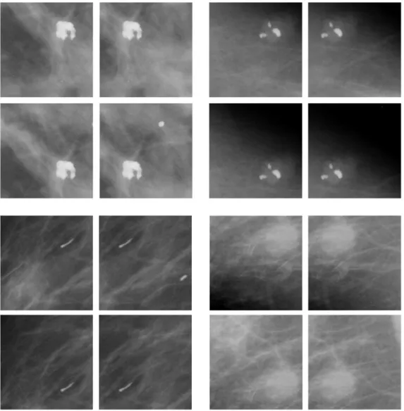
Figure 2. Example of CBIS-DDSM mammography images and ROI patches... 7
Figure 3. Illustration of the spatial property of kernel in convolution layer ... 9
Figure 4. Illustration of Pooling Operation ... 11
Figure 5. Illustration of an inception module with concatenation layer used in GoogLeNet ... 13
Figure 6. Illustration of Global Average Pooling applied on a RGB image ... 16
Figure 7. Raw image patches and normalized image patches ... 18
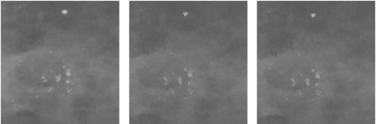
Figure 8. The raw microcalcification image patch , image with 2-magnitude elastic distortion, image with 4-magnitude elastic distortion... 19
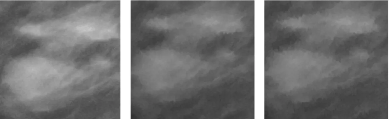
Figure 9. The raw mass image patch, image with 2-magnitude elastic distortion, image with 4-magnitude elastic distortion ... 20
Figure 10. Illustration of image coordination with cropping; augmented microcalcification image patches ... 21
Figure 11. Reference model of GoogLeNet cutted out for Class Activation Mapping .... 22
Figure 12. Illustration of modified GoogLeNet with Class Activation Map ... 23
Figure 13. Example of mammogram images with roughly held ROI masks ... 26
Figure 14. Full mammogram image for microcalcification , localization heatmap from reference model , localization heatmap for modified model and corresponding ROI mask images ... 28
LIST OF TABLES
Table 1. Size of training and testing image patches ... 18
Table 2. Size of training and testing image patches after data augmentation ... 21
Table 3.Modified GoogLeNet structure on 224x224 training patches ... 24
Table 4. IoU results for reference GoogLeNet and Modified GoogLeNet ... 25
Table 5. The intersection of detection results for reference GoogLeNet and Modified GoogLeNet ... 27
ABSTRACT
LOCALIZATION OF MICROCALCIFICATION ON THE MAMMOGRAM USING DEEP CONVOLUTIONAL NEURAL NETWORK
JIEUN JHANG 2018
Breast cancer is the most common cancer in women worldwide, and the mammogram is the most widely used screening technique for breast cancer. To make a diagnosis in the early stage of breast cancer, the appearance of masses and microcalcifications on the mammogram are two crucial indicators. Notably, the early detection of malignant microcalcifications can facilitate the diagnosis and the treatment of breast cancer at the appropriate time. Making an accurate evaluation on microcalcifications is a time-consuming and challenging task for the radiologists due to the small size and the low contrast of microcalcification. Compared to the background and mammogram image with noises, it is tough to be discriminated. Computer-Aided Detection (CADe) have been deployed to support radiologists. However, most of current CADe systems need to have hand-crafted image features to be implemented. For improvement in the
conventional approach, Convolutional Neural Network (CNN) with no hand-crafted image feature is used in this thesis. CNN with Class Activation Map (CAM) is deployed to implement the microcalcification detection in mammograms. GoogLeNet architecture with nine inception modules and one CAM layer is used to improve the localization capability of GoogLeNet in microcalcification detection while maintaining the local information. The network is trained and tested with Curated Breast Imaging Subset of Digital Database for Screening Mammography dataset (CBIS-DDSM). This approach
demonstrates that the localization ability of CAM for abnormal microcalcification regions on the mammogram can be improved by restoring the last two inception
modules that were removed in the paper [1] [16]. For the CAM, CAM layer is inserted in the position of the second auxiliary layer that was used in the original GoogLeNet [17] for training. This allowed us to use the intermediate feature at the same location from [1] [16] for localization while maintaining the depth of the GoogLeNet [17].
The experimental result shows that this method achieved about 225.15% better result at localizing microcalcification in mammograms than the existing method.
1 INTRODUCTION
According to the World Health Organization (WHO), cancer is one of the leading causes of death and breast cancer is the most common cancer in women worldwide [2].
Anatomically, the breast is composed primarily of fatty tissue with epithelium, ducts, and lobules connected with nutritional function.
Breast cancer is caused by excessive proliferation of these epithelial cells mainly in ducts and lobules; this proliferation usually causes lesions that can be detected and diagnosed by mammography. Without mammography, the probability of early detection is around only 5%. [11]
Mammography is the breast screening technology that the most commonly used in the world. Accurate abnormality detection plays a crucial role in mammography diagnoses. Early detection of cancer can be a critical factor in the future survival rate of cancer patients. [3] [4].
Moreover, mammography is universally recognized as the primary screening and diagnostic test that can be performed quickly and is the only test method for microcalcification detection, which may be one of the critical early findings of breast cancer [5]. A challenging issue is that it is often difficult and time-consuming for the radiologist to perform an accurate assessment of microcalcifications because of the small size and low contrast of microcalcification compare to the background of the
mammogram [6] [7]. Thus, computer-aided detection (CADe) have been introduced in mammography [8] [9].
Until recently, the performance of the CADe system was dependent upon hand-created features, designed and generated by radiologists. These features provide a platform which is task-specific and requires prior knowledge of experts, but they are highly biased towards how humans think and work [10].
Since the first introduction of artificial intelligence (AI) into the field of computer science, the research has seen the transition from rule-based or problem-based solutions to deep learning [11] [12] [13] [14].
Deep learning allows us to optimally exploit the ever-increasing amounts of data and reduce human bias. Its method is to extract information directly from training samples, rather than the extracted features from the domain expert. Many pattern recognition tasks have proven that the system is already reaching or leading to human performance [15].
In this thesis, based on the result from [1], the goal is aimed to improve the localization ability of CNN to detect suspicious microcalcification region in
mammograms using Class Activation Mapping (CAM). Using transfer learning, ImageNet pre-trained GoogLeNet is adapted as CNN architecture, and it is fine-tuned with cropped patches from CBIS-DDSM for mass, calcification, normal tissues and background. All the patches are resized into 224×224pixel size before being fed to train the CNN. Since the size of CBIS-DDSM dataset is too small to train the deep CNN, data augmentation is conducted to expand the volume of the dataset. One is elastic distortion, and another is image translation with cropping.
The CAM is used to detect the microcalcification region. Bolei Zhou et al. [16] adapted the CAM into GoogLeNet by removing the last two inception modules and
connect CAM convolution layer with global average pooling after it. By doing this, they maintain the local information from intermediate features with weight map generated after fully connected layer to implement the localization.
Due to the removal of the last two inception modules, the overall network loses its depth. Therefore, the network architecture is modified not to lose the depth while retaining the localization ability. The CAM layer is connected to full nine inception size GoogLeNet at the position of its second auxiliary layer. In this structure, the network can maintain the original depth of the GoogLeNet. The authors of GoogleNet claimed in the paper [17] that the auxiliary layer compensates for the disappearance of gradients during training. The CAM in this architecture then is expected to prevent the vanishing gradient problem while maintaining its localization capability, and it is assumed that it will enable localization to be more accurate as a deep structure than the CAM GoogLeNet from [16].
In the final step, full-size mammograms are used as input to evaluate the modified GoogLeNet and the GoogLeNet from the reference [1] [16]. Each
microcalcification localization displayed as a heatmap. Intersection over union (IoU) and the Intersection over Detection (IoD) will be deployed as evaluation methods.
2 RELATED WORK
2.1.MAMMOGRAPHY
Breast cancer is one of the major health problems in dealing with primary care. Mammography, Breast Ultrasonography, and Fine Needle Aspiration biopsy have been used to diagnose breast cancer. Digital mammography, Breast Magnetic Resonance Imaging (Breast MRI), Breast Computed Tomography scan (Breast CT), Positron Emission Tomography scan (PET), and early diagnosis using a Single-Photon Emission Computerized Tomography scan (SPECT) have been introduced. Among them,
mammography is a primary test for screening and diagnosis, and its effect is universally recognized [14][18]. Mammography is the primary screening and diagnostic test that can be performed very easily and is the only test method for visualizing microcalcification, which can be one of the critical early findings of breast cancer. [5]. Microcalcifications of the breast are commonly found in mammography and are especially common after
menopause [35]. Microcalcification is usually benign which means non-cancerous, but certain types of microcalcification or certain patterns of microcalcification may indicate precancerous changes in tissue or the breast cancer. [27] [28]. There are many
controversies over the effects of mammography. A false-positive result leads to an unnecessary biopsy, an increase in the mental anxiety of the examinee, and a relatively high false-negative rate of mammography for young women and dense breasts [21] [24]. In this thesis, I report that I have studied using only mammography images with the problems and the limitations of mammography mentioned above.
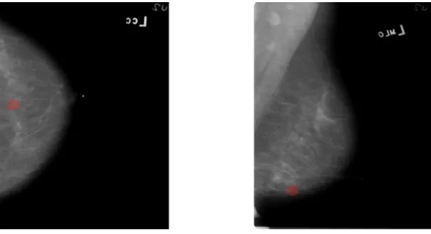
In the most cases, mammograms consist of two views of the breast, the
views for screening mammography. The CC view refers to the view from the head towards the breast in the vertical direction, and the MLO view refers to the view that tilt the breast about 45 degrees [20]. Figure 1 shows a mammogram of the same breast taken from MLO and CC views. Images are taken from CBIS-DDSM [19]. Red area indicates the same region of interest for the lesion with microcalcification.
Figure 1: Mammography with two views on the left chest of the same patient. Mammography is known to be less sensitive if the patient is young and if breast density is dense. [21] However, mammography is still the most representative primary breast cancer screening method.
2.2.CBIS-DDSM
In mammography, most researches are evaluated with private dataset due to the sensitivity for the privacy of medical data. With lack of a standard evaluation dataset available to the public, most of the published research results are difficult to replicate.
Digital Database for Screening Mammography (DDSM) [22] and
Mammographic Image Analysis Society (MIAS) database [23] were the most commonly used public dataset. DDSM was the most extensive public mammography database which collects more than 2500 mammographic images from Wake Forest University School of Medicine, Massachusetts General Hospital, Sacred Heart Hospital, and Washington University of St Louis School of Medicine. In each case, the region of interest (ROI) for microcalcification and mass is annotated with descriptions about mass shape, mass margin, calcification type, calcification distribution, and breast density [19]. In 2017, Lee et al. [19] released a curated, standardized version of the DDSM for the evaluation of CADe systems in mammography, CBIS-DDMS. The database contains 753 calcification cases and 891 mass cases. ROI cropping patches are included in each case with each view with full-size mammography and the resulting ROI mask image. Figure 2 shows full mammograms with its ROI patches. Images are taken from CBIS-DDSM [19]. The blue rectangles on left images are the ground truth bounding boxes that indicate the ROI mask area from CBIS-DDSM.
Figure 2. Example of CBIS-DDSM mammography images(left) and ROI patches(right)
2.3.COMPUTER-AIDED DETECTIONS
Microcalcifications are one of the most crucial early symptom appearances on mammograms [35]. Their diameter is mostly less than 1mm and constructed with small deposits of calcium that appear as bright little spots on mammograms [25] [26] [27] [36]. Pal et al. [28] introduced a multilevel system that detects microcalcifications using neural networks in mammography. The authors located the candidate calcification area, configured the network output to remove thin, slender structures and used local density for final classification. Wang et al. [29] applied Stacked Autoencoder (STA) constructed
with two convolutional layers after image segmentation to classify the malignancy of microcalcifications and masses. 15 segmented image features used for
microcalcifications and 26 for masses. Then they combined all 41 features for
classification. Tabar et al. [30] used a learning approach to extract local features for the shape of microcalcifications and then selected the most prominent features for use in the classifier.
Mass detection algorithms first detect suspicious regions in a mammogram and then classify the malignancy. Petrick et al. [10] used Laplacian Gaussian for edge detection and contrast-emphasis filters using adaptive weights to discriminate the potential mass. Morphological features were extracted to classify normal and mass ROI. Cascio et al. [31] first used the edge-based approach to refine the boundaries of the ROI and then computed the geometric features. Neural networks have been trained to
distinguish between mass and normal areas.
Previous classifiers mainly used shallow neural networks as classifiers and used hand-crafted features when performing computer-aided detection, but in recent years, many studies have been done by applying deep learning into CADe.
2.4.DEEP CONVOLUTIONAL NEURAL NETWORK ARCHITECTURE
2.4.1 CONVOLUTIONAL NEURAL NETWORK
Convolutional neural network (CNN) is a neural network, specialized for processing a grid-like topology data such as the image, which is a 2-dimensional grid of pixels.
Convolution is a linear operation on two functions with some variable 𝑡.
Convolution is to reverse and shift one of the functions 𝑓 and 𝜔, and then to integrate the result of the multiplication with the other function:
s(𝑥) = (𝑓 ∗ 𝜔)(𝑥) s(𝑥) = ∫ 𝑓(𝑡)𝜔(𝑥 − 𝑡)𝑑𝑡
∞ −∞
in which, 𝑓(𝑥) is the output of the function 𝑓, and 𝜔(𝑡) is a weighting function for convolution in CNN. Convolution is defined for all functions defined by the above integral function for any purposes. [38]
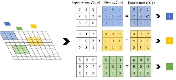
In convolutional neural networks, 𝑓(𝑥) is referred to as the input, 𝜔(𝑡) is referred to as the kernel and the output s(𝑥) is referred to as the feature map. The input is usually a multidimensional array data (e.g., an image), and the kernel is a
multidimensional array of parameters that are intended to converge with the learning algorithm. Figure 3 shows this spatial property of convolution layer.
The following three ideas improve the learning algorithm of CNN: Sparse interaction, parameter sharing, equivariant representations [38].
Even if the input could consist of thousands of pixels, we intentionally keep the network’s kernel small. The resulting network not only ‘sees’ the relevant features such as an edge, but also lessen the required computation and ameliorate statistical efficiency. This is the advantage and the attribute of sparse interaction or connectivity from CNN.
The parameter sharing scheme allows CNN to control and reduce the number of parameters. If each convolution layer uses a different weight for each neuron location at all depth, the number of parameters is very high. Rather than using this enormous number of parameters, take the advantage from the simple assumption that if one feature is useful for computation at some spatial location, it should be useful to compute at another
location. In other words, the neurons of each depth slice use the same weights and bias by limiting the number of neurons at each depth slice (dimensional slice used in
2-dimensional image processing). During backpropagation, every neuron in the input volume computes the gradients for its weights, and then the gradients are summed over each depth slice. Finally, it updates only one set of weights per depth slice. The forward pass of the convolution layer can be computed as the convolution of the weights of the
neurons with input volume at each depth slice. Therefore, we name the set of weights as a filter (or kernel).
A function h is said to be equivariant to a function g if h and g satisfy the following property:
ℎ(𝑔(𝑥)) = 𝑔(ℎ(𝑥))
Let h denotes the function that shifts every pixel to the right and g the function that modifies the brightness of a pixel at coordinates (𝑥, 𝑦). The parameter sharing enables us to say that if we applied h to the convolution and we applied the convolution to the result of h, both computations are equal. In other words, if we move an object in a specific image, its representation does not change. This is particularly interesting in dealing with images, since the equivalence renders CNN invariant to the horizontal/vertical
translation. This is the reason that CNN is said to possess a property called ‘equivariant representation’.
The pooling operation renders the network invariant, in a certain way, to small translations of the input. Provided that the underlying assumption is correct, this
characteristic gives the network another tool for the statistical efficiency.
Figure 4 illustrates how a max pooling (with filter size 2 × 2 and stride 2) works. The operation aims to get the maximum pixel value, ‘pool’ the value and the resulting image’s resolution’s 50% reduced.
2.4.2 DEEP LEARNING
The primary function of deep learning aims to approximate a function 𝑦 = 𝑓(𝑥: 𝜃), where the function maps an input x to a label y and 𝜃 = ⋃ 𝜃𝑖 is a collection of
parameters 𝜃𝑖 in a neural network. The main difference of the deep learning lies in the assumption that f is to be approximated by a set of 𝑓(𝑖) functions:
𝑓(𝑥) ≈ 𝑓(𝑛)°𝑓(𝑛−1)° … °𝑓(2)°𝑓(1)(𝑥)
, where º is the composition operator. In this case, 𝑓(1), 𝑓(2), …, 𝑓(𝑛) denote respectively the i-th (1 ≤ 𝑖 ≤ 𝑛) layer of a neural network and the overall length of a network,
denoted by n, is the depth of a neural network. During the training of a neural network, we adjust the set of parameters to approximate 𝑓(𝑥), in a numerical fashion.
2.4.3 GOOGLENET
ImageNet [33] is one of the most extensive, public datasets in image recognition work and plays a significant role in object classification and detection. The project now consists of more than 14 million images, categorized as more than 20,000 classes, with objects in the middle of the image that classify the class. This effort for labeling a
year, the ImageNet Large Scale Visual Recognition Challenge (ILSVRC) is held to select the best performing architecture and training strategies of the year [34].
Szegedy et al. [17] introduced a deeper CNN, GoogLeNet to ILSVRC-2014 and winning the competition. Instead of sequential stacking of layers, this network used parallel structure in the architecture using the inception modules.
Inception module is an amalgam of a series of the convolutional filters of
different sizes; it concatenates different size filters and dimensions into a single new filter to obtain features of different scales [37]. In addition, 1 × 1 convolution is appropriately used to reduce the dimension and solve the problem of increasing the computation amount when the network is deepened [26]. Each inception unit in GoogLeNet consists of six convolution layers and one pooling layer. GoogLeNet used Global Average Pooling (GAP) at the final convolutional layer. When the network identifies all the discriminating areas of an image, using average pooling rather than maximum pooling is more profitable in terms of feature loss.
During the training period, only the following two inception modules after Class Activation Mapping modules are fine-tuned. Training is done with CBIS - DDSM dataset whose batch size of 16. Each of network iterated 200 epochs with Imagenet pre-trained weights. If the average accuracy for the 50 most recent deployments reaches 99.5%, each network will stop from further training. The learning rate set to 1e-4 for the initial state. Each architecture is trained and saved five times, and the average localization result of five models is deployed for the robustness of evaluation
2.5.CLASS ACTIVATION MAP
Class Activation Mapping (CAM) is a technology that uses a specific class of CNN to identify regions of an image [16]. The CAM can identify image areas associated with a given class and reuse the classifiers for localization. It shows that CNN has the built-in, detection capability. If CNN classifies the input image with a high degree of accuracy, it can be considered that the classifier has learned to filter for the class.
Conversely, by navigating back to the location where the weights of the filter are active, they will indicate the location where the class is in that image.
For a given image, let 𝑓𝑖(𝑥, 𝑦) represent the activation of unit i in the last
convolutional layer at a spatial location (𝑥, 𝑦). Then, for unit 𝑘, the result of performing global average pooling, 𝐹𝑘 is s
∑𝑥,𝑦𝑓𝑘(𝑥, 𝑦).
Therefore, for a given class 𝑐, the input to the softmax, 𝑆𝑐, is ∑ 𝑤𝑖 𝑖𝑐𝐹𝑖 where 𝑤𝑖𝑐
is the weights corresponding to class 𝑐 for unit i. Essentially, 𝑤𝑖𝑐 indicates the importance of 𝐹𝑖 for class 𝑐.
𝑆𝑐 = ∑ 𝑤𝑘𝑐 𝑘 ∑ 𝑓𝑘(𝑥, 𝑦) 𝑥,𝑦 = ∑ ∑ 𝑤𝑘𝑐𝑓𝑘(𝑥, 𝑦) 𝑘 𝑥,𝑦
Let ω𝑖 (𝑖 = 1, 2, . . . , 𝑛) denote weights at the output layer and 𝑓𝑖(𝑥, 𝑦) (i = 1, 2, . . . , 𝑛) the output of the last convolutional layer, computed by the activation mapping 𝑓𝑖, at the spatial location of certain pixel coordinates (𝑥, 𝑦). Denote the set of
classes by 𝐶. Then, CAM can be represented as follows:
CAM = ∑ ∑ 𝜔𝑖𝑐𝑓𝑖
𝑛
𝑖=1 𝑐∈𝐶
(𝑥, 𝑦)
The resulting CAM is then displayed for visualization and further verification purpose. The authors of [16] claimed that the CNN could learn the importance of the regions by projecting back the weights onto convolutional feature maps.
Xi et al. [1] trained the neural network using image patches from CBIS-DDSM and tested its localization capability on full mammograms with Class Activation Map. They cut out the last two inception modules from GoogLeNet and connect CAM
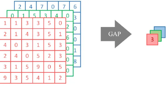
convolutional layer with Global Average Pooling layer (GAP layer) right after it. Global Averaging Pooling is a pooling that performs an entire input volume as a target and generates the average value of the entire input volume as output.
Figure 6. Illustration of Global Average Pooling applied on a RGB image During Class Activation Mapping, the point at which the largest pooling occurs in the network is the GAP layer at the last CAM convolution layer. It may maintain local information from intermediate filters, but it loses too much information at a time.
Moreover, because the authors of [1] truncate the last two modules, the depth of the network becomes shallower than the original network.
In order to maintain the depth of the network without compromising the functionality of GAP (Global Average Pooling), which plays a crucial role in CAM, the CAM layer is connected to full nine inception size GoogLeNet at the position of its auxiliary layer.
3. METHODOLOGY
3.1. PREPROCESSING
Prior to training the machine, since all CBIS-DDSM data are compressed in Digital Imaging and Communications in Medicine (DICOM) format, only mammography images of each patient are extracted as Portable Network Graphics (PNG) files. The DICOM format is an industry-wide, standard format that contains medical imaging data as well as a series of interdependent information entities [27]. Each entity contains data that includes specific aspects of the actual process (e.g., the process of image acquisition, printing) and related physical objects (e.g., patient information, characteristic of the lesion, image format). [32]
Since each mammogram in the dataset can have a wide range of image intensities, mammogram preprocessing is paramount. The intensity of each mammogram can vary greatly depending on the X-ray machine used, the density of the patient's breast tissue, the institution that took the mammograms, and various other peripheral factors.
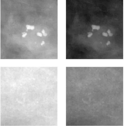
Therefore, normalization on the entire dataset serves each feature to have a similar intensity range in order to obtain the stable gradients. This normalization is implemented by subtracting the mean value of the entire data set for each image. Figure 7 shows the raw ROI image patches and normalized image patches for microcalcification of CBIS-DDSM dataset. In the case of microcalcifications, many mammograms contain a certain amount of mass, also.To distinguish these two abnormalities, two classes of mass and microcalcification are labeled using the CBIS-DDSM training set. These two classes are used in the reference model for their binary classification scheme [1].
Figure 7. Raw image patches (left) and normalized image patches (right) In addition to mass and microcalcification, two classes of normal tissue and background were added to allow the network to learn more specific localization. Table 1 shows the quantitative composition of image patches from CBIS-DDSM with four classes.
Class Training Testing Overall
Microcalcification 1546 326 1872
Mass 1318 378 1696
Normal tissue 1502 380 1882 Background 1444 352 1796
3.2. DATA AUGMENTATION
To avoid the overfitting during training, several data augmentation is applied to cropped images from CBIS-DDSM such as elastic augmentation and image translation.
Elastic distortion is a method developed by Microsoft® for effective training data generation. It is patented by Microsoft. This method produces a displacement vector in various directions and produces a more complex form of augmented data through it.
However, elastic deformation has been discarded because it was found that it deformed the image features of mass and calcification too much. Particularly in the case of microcalcification, due to its small size (the diameter of microcalcification is mostly less than 1 mm), the features may change too much even with very weak elastic
distortion magnitude. Even for the case of mass, since the outline of mass is one of the crucial factors to determine the malignancy of mass on mammography, elastic distortion is not a proper way to augment data. Figure 8 and Figure 9 show the sample images that show the effect of elastic distortion for mass and calcification features.
Figure 8. The raw microcalcification image patch (left), image with 2-magnitude elastic distortion(middle), image with 4-magnitude elastic distortion(right)
Figure 9. The raw mass image patch(left), image with 2-magnitude elastic distortion(middle), image with 4-magnitude elastic distortion(right)
For the machine to learn all the image properties in the kernel window, image translation is conducted.
Image translation is adapted to allow the network to learn the images with a lesion in various directions besides the image where the object is located at the center of the image patch. For this purpose, CBIS-DDSM full-size mammography images and corresponding mask images used to create ROI locations for entire training data, resulting in new image patches with ROIs in the northwest, northeast, southeast, and southwest side of each image. The sample image patches of microcalcification for image translation with cropping are shown in Figure 10.
Moreover, due to the vast size difference exists in image patches of CBIS-DDSM, for image patches that the image size is less than 224 pixels × 224 pixels, I created the larger image patches containing the surrounding area by loosening the ROI boundaries.
Additional normal tissue and background image patches are added to the
training data to maintain the data ratio of each class. The number of training dataset after data augmentation are listed in table 2.
Figure 10. Illustration of image tranclastion with cropping; augmented microcalcification image patches
Class Training Testing Overall
Microcalcification 7872 326 8198
Mass 6636 378 7014
Normal tissue 7510 380 7890 Background 7220 352 7572 Table 2. Size of training and testing image patches after data augmentation
3.3. NETWORK ARCHITECTURE
The training is conducted on the following setting: Intel® i7-3700 @ 3.40 GHz, 24 Gb Ram, a single Nvidia® GTX 1080, Ubuntu 16.04 and Caffe framework. Each training takes about 60-80 minutes to be completed. For training, the learning rate set to 1e-4 and the weight decay rate set to 0.0005. For both reference and modified model, the iteration for training is set to 200 epochs. If the average accuracy for the 50 most recent deployments reaches 99.5%, each network will stop from further training. These settings are identical to the experimental conditions of the reference model, which allowed me to simulate the reference model in an identical environment. All the results and models are examined 5 times to get the statistic robustness. The entire preprocessed image patches are resized to 224x224 pixels for training, and the entire full-size mammography images are resized to 3000x3000 pixels for testing. However, since the testing image is vast, Global Average Pooling (GAP) loses too much information to maintain local information in the intermediate feature with the referenced CNN model [1] [16].
In my methodology, the 187x187 pixel sized 1024 features are flattened into 1x1 size at once with test images. To overcome this issue, removed 2 inception modules are
connected after Class Activation Mapping (CAM) occurred. CAM then inserted in the way that the auxiliary layer of GoogLeNet was inserted.
Figure 12. Illustration of modified GoogLeNet with Class Activation Map The authors of Google Net claimed in the paper [17] that the auxiliary layer compensates for the disappearance of gradients during training. With this modified network
architecture, the class activation map is expected to play this role with its localization capability, and it is assumed that the following two inception modules will enable
localization to be more accurate as a deep structure. The threshold value for the bounding box is set to 0.9. This means that the boundary is selected by the position of the most active weight of the top 10%. The modified map is constructed with nine inception modules.
Type size/stride Patch Output size
Output of convolution layers in the inception module #1x1 (1x1) #3x3 reduce (1x1) #3x3 (3x3) #5x5 reduce (1x1) #5x5 (5x5) pooling Convolution 7 × 7/2 112 × 112 × 64 Max pooling 3 × 3/2 56 × 56 × 64 Convolution 3 × 3/1 56 × 56 × 192 64 192 Max pooling 3 × 3/2 28 × 28 × 192 Inception 1 28 × 28 × 256 64 96 128 16 32 32 Inception 2 28 × 28 × 480 128 128 192 32 96 64 Max pooling 3 × 3/2 14 × 14 × 480 Inception 3 14 × 14 × 512 192 96 208 16 48 64 Inception 4 14 × 14 × 512 160 112 224 24 64 64 Inception 5 14 × 14 × 512 128 128 256 24 64 64 Inception 6 14 × 14 × 528 112 144 288 32 64 64 Inception 7 14 × 14 × 832 256 160 320 32 128 128 CAM convolution 3 × 3/1 1 × 1 × 1024 Global Average Pooling 187 × 187/2 1 × 1 × 1024 Linear 1 × 1 × 1024 Softmax 1 × 1 × 4 Max pooling 3 × 3/2 7 × 7 × 832 Inception 8 7 × 7 × 832 256 160 320 32 128 128 Inception 9 7 × 7 × 1024 384 192 384 48 128 128 Global Average Pooling 7 × 7/1 1 × 1 × 1024 Dropout (40%) 1 × 1 × 1024 Linear 1 × 1 × 4 Softmax 1 × 1 × 4
4. RESULTS AND EVALUATION
Evaluation of localization is done by the Intersection over Union (IoU). This metric computes the ratio of the intersection of two bounding boxes over the union, one given by the classifier and the other the ground truth. The more its value is close to 1, the more accurate the classifier is. Given two bounding boxes A and B, we have:
IoU(𝐴, 𝐵) =|𝐴 ∩ 𝐵| |𝐴 ∪ 𝐵|=
|𝐴 ∩ 𝐵| |𝐴| + |𝐵| − |𝐴 ∩ 𝐵|
, where |∙| denotes the area bounded by the box.
The bounding box will cover the
Model Average IoU for microcalcification detection
Modified GoogLeNet with CAM 0.146
Reference GoogLeNet with
CAM 0.136
Table 4. IoU results for reference GoogLeNet and Modified GoogLeNet As shown in Table 4, the average IoU value is very low for both the main reference network and the modified network, although the value of the modified network shows slightly better results. The reason for this low IoU value is because the ROI ground truth for CBIS-DDSM is sometimes too large and too roughly held. Lee et al. claims [19] that the ROI annotations for DDSM anomalies are provided to indicate the general location of the lesion, but not the accurate location. Therefore, many researchers need to implement a segmentation algorithm for accurate feature extraction with domain
experts. Direct comparison of the performance of methods or replicate previous results are not possible. This issue reduced the average of IoU value from the modified model which try to achieve more precise localization. Figure 13 shows the example of roughly held ROI masks. As you can see, some of the masks are very large enough to cover the outer part of the breast, and others are huge enough to cover the entire breast.
Since the IoU value is not the best way to evaluate localization with these roughly measured ground truths, this thesis focuses on the most strongly activated regions among all the ROI candidates that estimated by the network.
The intersection between ground truth areas and detected areas are divided by the areas of detection.
𝐼𝑛𝑡𝑒𝑟𝑠𝑒𝑐𝑡𝑖𝑜𝑛𝑜𝑣𝑒𝑟𝐷𝑒𝑡𝑒𝑐𝑡𝑖𝑜𝑛 (𝐼𝑜𝐷) (⋃ 𝑅𝑖 𝑚 𝑖=1 , ⋃ 𝐺𝑗 𝑛 𝑗=1 ) = ∑| ∑ 𝑅𝑖 𝑚 𝑖=1 ∩ 𝐺𝑗| | ∑𝑚𝑖=1𝑅𝑖| 𝑛 𝑗=1
, where | ∙ | denotes the area bounded by the box, 𝑛 is the number of ROI candidate bounding boxes with a threshold, 𝑅𝑖is the area of each 𝑛 ROI candidates, 𝑚 is
the number of all the ground truth bounding boxes and 𝐺𝑗 is each ground truth bounding box area.
The more its value is close to 1, the more detection areas intersect with the ground truth. In other words, the more its value is close to 0, the more the occurrence of the false positive detection increases. The network fails to detect the ROI area when the intersection over detection value reached 0.
Model Average IoD for microcalcification detection
Modified GoogLeNet with CAM 0.367 Reference GoogLeNet with CAM 0.163
Table 5. The intersection of detection results for reference GoogLeNet and Modified GoogLeNet
Figure 14. Full mammogram for microcalcification (first column), localization heatmap from reference model (second column), localization heatmap for the modified model
Figure 14 shows the results of microcalcification localization from the referenced model and the modified model. The first column of Figure 14 shows the original mammograms from CBIS-DDSM, resized to 3000 × 3000 pixel size. The second column is the images of the localization results of the reference model converted into the heatmap images, and the third column shows the localization results of the modified model as the heatmap images. The closer the color of the heatmap is blue, the more weights are not activated, and the closer the heatmap color is red, the more weights are activated. Thus, the area marked in red indicates the location of the specified class object. Finally, the last column is the mask images from CBIS-DDSM corresponds to each image from the first column. As you can see, a large number of false positive areas are detected in the reference model. However, in the resulting heatmap of the modified model, it performs more elaborate localization, which intersects to the ground truth region with much less false positive alarms.
5. CONCLUSION
Due to the absence of the supervision of experts for image segmentation, this thesis could not yield highly sophisticated evaluation results. However, the inspection of visual images and various numerical indicators (e.g., IoU and IoD) confirmed that the modified model has a better localization ability for microcalcification than the existing GoogleNet with CAM. The evaluation results are generally lower than the average of image localization (≥ 50%), which is considered a general threshold, but it can be easily improved if more sophisticated ROI ranges can be obtained under the supervision of the domain expert as described above. In numerical terms, the modified model showed about 225.15% better localization result than the reference model for an average of Intersection of Detection value for the entire testing data, and about 7.4% better in the average of the Intersection of Union value.
Computer-Aided Detection (CADe) have been deployed to support radiologists for mammography diagnosis. However, most of current CADe systems need to have crafted image features that generated from domain experts. In this thesis, no hand-crafted image features were used. CNN with Class Activation Map (CAM) shows that the localization of microcalcification can be implemented with much less human effort. These results show that a network which can localize the sophisticated area of microcalcifications can be implemented to support the radiologists.
6. LITERATURE CITED
1. Xi, P., Shu, C., & Goubran, R. (2018). Abnormality Detection in Mammography
using Deep Convolutional Neural Networks. arXiv preprint arXiv:1803.01906
2. Roth, Holger R., et al. "Improving computer-aided detection using convolutional
neural networks and random view aggregation." IEEE transactions on medical imaging 35.5 (2016): 1170-1181.
3. Tabar, L., Yen, M. F., Vitak, B., Chen, H. H. T., Smith, R. A., & Duffy, S. W. (2003).
Mammography service screening and mortality in breast cancer patients: 20-year follow-up before and after introduction of screening. The Lancet, 361(9367), 1405-1410.
4. Broeders, M., Moss, S., Nyström, L., Njor, S., Jonsson, H., Paap, E., ... & Paci, E.
(2012). The impact of mammographic screening on breast cancer mortality in Europe: a review of observational studies. Journal of medical
screening, 19(1_suppl), 14-25.
5. Bomalaski, J. J., Tabano, M., Hooper, L., & Fiorica, J. (2001). Mammography.
Current Opinión in Obstetrics and Gynecology, 13(1), 15-23.][ Fletcher, S. W., & Elmore, J. G. (2003). Mammographic screening for breast cancer. New England Journal of Medicine, 348(17), 1672-1680.
6. Goergen, S. K., Evans, J., Cohen, G. P., & MacMillan, J. H. (1997). Characteristics
of breast carcinomas missed by screening radiologists. Radiology, 204(1), 131-135.
7. Barlow, W. E., Chi, C., Carney, P. A., Taplin, S. H., D’orsi, C., Cutter, G., ... &
characteristics of radiologists. Journal of the National Cancer Institute, 96(24), 1840-1850.
8. Li, Y., Chen, H., Cao, L., & Ma, J. (2016). A survey of computer-aided detection of
breast cancer with mammography. J. Health Med. Inform, 7(4).
9. Tang, J., Rangayyan, R. M., Xu, J., El Naqa, I., & Yang, Y. (2009). Computer-aided
detection and diagnosis of breast cancer with mammography: recent advances. IEEE Transactions on Information Technology in Biomedicine, 13(2), 236-251.
10. Kooi, T., Litjens, G., van Ginneken, B., Gubern-Mérida, A., Sánchez, C. I., Mann,
R., ... & Karssemeijer, N. (2017). Large scale deep learning for computer aided detection of mammographic lesions. Medical image analysis, 35, 303-312.
11. Bengio, Y. (2009). Learning deep architectures for AI. Foundations and trends® in
Machine Learning, 2(1), 1-127.
12. Bengio, Y., Courville, A., & Vincent, P. (2013). Representation learning: A review
and new perspectives. IEEE transactions on pattern analysis and machine intelligence, 35(8), 1798-1828.
13. Schmidhuber, J. (2015). Deep learning in neural networks: An overview. Neural
networks, 61, 85-117.
14. LeCun, Y., Bengio, Y., & Hinton, G. (2015). Deep learning. nature, 521(7553), 436. 15. CireşAn, D., Meier, U., Masci, J., & Schmidhuber, J. (2012). Multi-column deep
neural network for traffic sign classification. Neural networks, 32, 333-338.
16. Zhou, B., Khosla, A., Lapedriza, A., Oliva, A., & Torralba, A. (2016). Learning deep
features for discriminative localization. In Proceedings of the IEEE Conference on Computer Vision and Pattern Recognition (pp. 2921-2929).
17. Szegedy, C., Liu, W., Jia, Y., Sermanet, P., Reed, S., Anguelov, D., ... & Rabinovich,
A. (2015). Going deeper with convolutions. In Proceedings of the IEEE conference on computer vision and pattern recognition (pp. 1-9).
18. Drake, R., Vogl, A. W., & Mitchell, A. W. (2009). Gray's Anatomy for Students
E-Book. Elsevier Health Sciences.
19. Lee, R. S., Gimenez, F., Hoogi, A., Miyake, K. K., Gorovoy, M., & Rubin, D. L.
(2017). A curated mammography data set for use in computer-aided detection and diagnosis research. Scientific data, 4, 170177.
20. Andersson, I., Ikeda, D. M., Zackrisson, S., Ruschin, M., Svahn, T., Timberg, P., &
Tingberg, A. (2008). Breast tomosynthesis and digital mammography: a comparison of breast cancer visibility and BIRADS classification in a population of cancers with subtle mammographic findings. European radiology, 18(12), 2817-2825.]
21. Carney, P. A., Miglioretti, D. L., Yankaskas, B. C., Kerlikowske, K., Rosenberg, R.,
Rutter, C. M., ... & Cutter, G. (2003). Individual and combined effects of age, breast density, and hormone replacement therapy use on the accuracy of screening
mammography. Annals of internal medicine, 138(3), 168-175.
22. Heath, M., Bowyer, K., Kopans, D., Kegelmeyer, P., Moore, R., Chang, K., &
Munishkumaran, S. (1998). Current status of the digital database for screening mammography. In Digital mammography (pp. 457-460). Springer, Dordrecht
23. Suckling, J., Parker, J., Dance, D., Astley, S., Hutt, I., Boggis, C., ... & Taylor, P.
(1994, July). The mammographic image analysis society digital mammogram database. In Exerpta Medica. International Congress Series (Vol. 1069, pp. 375-378).
24. Saarenmaa, I., Salminen, T., Geiger, U., Heikkinen, P., Hyvärinen, S., Isola, J., ... &
Kärkkäinen, A. (2001). The effect of age and density of the breast on the sensitivity of breast cancer diagnostic by mammography and ultasonography. Breast cancer research and treatment, 67(2), 117-123.
25. American College of Radiology, & American College of Radiology. (2003). Breast
Imaging Reporting and Data System Atlas (BI-RADS® Atlas) Reston. VA: American College of Radiology, 1-259.
26. Winchester, D. P., Jeske, J. M., & Goldschmidt, R. A. (2000). The diagnosis and
management of ductal carcinoma in‐situ of the breast. CA: a cancer journal for clinicians, 50(3), 184-200.
27. Schreer, I., & Lüttges, J. (2005). Breast cancer: early detection. In
Radiologic-Pathologic Correlations from Head to Toe (pp. 767-784). Springer, Berlin, Heidelberg.
28. Pal, N. R., Bhowmick, B., Patel, S. K., Pal, S., & Das, J. (2008). A multi-stage
neural network aided system for detection of microcalcifications in digitized mammograms. Neurocomputing, 71(13-15), 2625-2634
29. Wang, J., Yang, X., Cai, H., Tan, W., Jin, C., & Li, L. (2016). Discrimination of
breast cancer with microcalcifications on mammography by deep learning. Scientific reports, 6, 27327.
30. Tabar, L., Yen, M. F., Vitak, B., Chen, H. H. T., Smith, R. A., & Duffy, S. W. (2003).
Mammography service screening and mortality in breast cancer patients: 20-year follow-up before and after introduction of screening. The Lancet, 361(9367), 1405-1410.
31. Pal, N. R., Bhowmick, B., Patel, S. K., Pal, S., & Das, J. (2008). A multi-stage
neural network aided system for detection of microcalcifications in digitized mammograms. Neurocomputing, 71(13-15), 2625-2634
32. Gueld, M. O., Kohnen, M., Keysers, D., Schubert, H., Wein, B. B., Bredno, J., &
Lehmann, T. M. (2002, May). Quality of DICOM header information for image categorization. In Medical Imaging 2002: PACS and Integrated Medical Information Systems: Design and Evaluation (Vol. 4685, pp. 280-288). International Society for Optics and Photonics.
33. Deng, J., Dong, W., Socher, R., Li, L. J., Li, K., & Fei-Fei, L. (2009, June).
Imagenet: A large-scale hierarchical image database. In Computer Vision and Pattern Recognition, 2009. CVPR 2009. IEEE Conference on (pp. 248-255). Ieee.
34. Russakovsky, O., Deng, J., Su, H., Krause, J., Satheesh, S., Ma, S., ... & Berg, A. C.
(2015). Imagenet large scale visual recognition challenge. International Journal of Computer Vision, 115(3), 211-252.
35. Lai, K. C., Slanetz, P. J., & Eisenberg, R. L. (2012). Linear breast calcifications.
American Journal of Roentgenology, 199(2), W151-W157.
36. Demetri-Lewis, A., Slanetz, P. J., & Eisenberg, R. L. (2012). Breast calcifications:
the focal group. American Journal of Roentgenology, 198(4), W325-W343.
37. Lin, M., Chen, Q., & Yan, S. (2013). Network in network. arXiv preprint
arXiv:1312.4400.
38. Goodfellow, I., Bengio, Y., Courville, A., & Bengio, Y. (2016). Deep learning (Vol.