Distributed deep neural networks

Copyright

by

Subhash Venkat Mullapudi

2017

The Report Committee for Subhash Venkat Mullapudi

Certifies that this is the approved version of the following report:

Distributed Deep Neural Networks

APPROVED BY

SUPERVISING COMMITTEE:

Constantine, Caramanis

Sarfraz, Khurshid

Supervisor:

Distributed Deep Neural Networks

by

Subhash Venkat Mullapudi

Report

Presented to the Faculty of the Graduate School of

The University of Texas at Austin

in Partial Fulfillment

of the Requirements

for the Degree of

Master of Science in Engineering

The University of Texas at Austin

December 2017

Dedication

I dedicate this report to my loving family and friends, who helped me soar this high. I ran

out of time to search for something clever on the internet, but insert meme here. I also

dedicate this report to the future me - you did this, you could have had more planning and

inserted a good joke but no.

Abstract

Distributed Deep Neural Networks

Subhash Venkat Mullapudi, M.S.E

The University of Texas at Austin, 2017

Supervisor: Constantine, Caramanis

Deep neural networks have become popular for solving machine learning

problems in the field of computer vision. Although computers have reached parity in the

task of image classification in machine learning competitions, the task of mining massive

training data often takes expensive hardware a long time to process. Distributed protocol

for model training can be attractive because less powerful distributed nodes are cheaper

to operate than specialized high-performance cluster. Stochastic gradient descent (SGD)

is a popular optimizer at the heart of many deep learning systems. To investigate the

performance of distributed asynchronous SGD, Tensorflow deep learning framework was

tested with Downpour SGD and Delay Compensated SGD to see effect of model training

in typical commercial environments. Experimental results show that both Downpour and

Delay Compensated SGD are viable protocols for distributed deep learning.

Table of Contents

List of Tables ... vii

List of Figures ... viii

Introduction ...1

Mathematical Concepts for Deep Learning ...7

Linear Classifier ...7

Loss Function ...8

Regularization ...9

Stochastic Gradient Descent ...9

Neuron model...13

Softmax function ...13

Forward/Backward propagation ...14

Dropouts ...14

Activation function ...15

Max Pooling, shared weights, local receptive fields...17

Neural Network architectures ...17

Convolutional Neural Networks ...18

Downpour SGD ...21

Delay Compensation SGD ...22

TensorFlow ...22

Experiment ...26

Conclusion ...30

Appendix ...31

References ...33

List of Tables

Table 1: Google Cloud pricing for computing instances ...27

Table 2: Average run time per node ...29

List of Figures

Figure 1: Abstract graph which highlights performance advantage of deep learning

over traditional methods in image classification competitions ...2

Figure 2: Graph depicting hours of practice vs Score for a sample of students ...7

Figure 3: Graph depicting the convergence of SGD algorithm to solution ...11

Figure 4: Simplified biological neuron model ...13

Figure 5: Comparison of Standard Neural Net before and after applying dropout15

Figure 6: Sigmoid function

σ

(

x

)=1/(1+

e

−x

) with a range between 0 and 1

...15

Figure 7: Tanh function tanh(x) with a range between -1 and 1 ...16

Figure 8: ReLU function which activates when x>0 and responds with linear function

...16

Figure 9: Theoretical relationships between different layers of neural network ...18

Figure 10: Convolutional Neural Network architecture Lenet 5 for MNIST dataset19

Figure 11: AlexNet Architecture ...19

Figure 13: Downpour SGD model ...21

Figure 14: Relationship between workers and Global model ...22

Figure 15: TensorFlow hardware and software stack ...24

Introduction

Artificial Neural Networks (ANNs), under the broad field of Artificial Intelligence (AI), is an active area of research with wide impact across multiple disciplines. Historically, AI research goes through active and dormant phases which Nilsson in “Quest for Artificial Intelligence” [1] calls AI summer or winter. The current AI summer phase has renewed interest in ANNs, especially for the fields of computer vision, natural language processing and robotics. One inflection point for the current summer AI was is 2012, when Hinton [2] swept popular machine learning competitions with his innovative ANNs. Hardware capabilities, like cheap memory storage, increased processing power, etc. contributed to the current summer AI, but this report will focus on the software algorithms needed to scale ANNs in commercial environments. This report will explore distributed model training for ANNs which remains a stubborn problem.

Deep learning is a popular phrase for the current generation of ANNs because the term ‘deep’ emphasizes the importance of network depth in the ANNs. In research literature and common parlance the terms ANNs or deep learning are often used interchangeably. The first part of this report will cover the recent advances in ANNs and their impact, second part will review relevant mathematical concepts for constructing ANNs, and the final section will cover experiment and discussion of distributed deep learning.

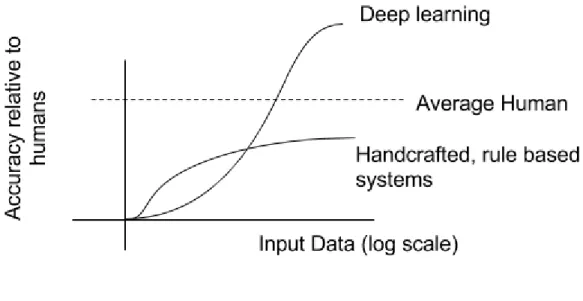
Before Hinton’s contribution, most AI programmers spent painstaking programming hours to handcraft algorithmic features to achieve performance. However, ANNs allow for automated generation of models/parameters based on large datasets often with noisy analog data or

unstructured datasets. ANNs tend to scale better with larger data, unlike previous methods which often plateau in performance after a certain dataset size. One overarching way to characterize previous methods in AI, is that programmers enforced a logical rule-based system where humans extracted features, created custom models, and tuned models till output satisfied expectations [1]. One-way ANNs are distinct from previous methods in AI, is their ability to automated feature extractions from larger datasets which are fed through automatically via network which tune parameters until output matches expectations.

Figure 1: Abstract graph which highlights performance advantage of deep learning over

traditional methods in image classification competitions

The computer vision field often grows lockstep with AI, and in this new era of deep learning has experienced rapid advancement for the task of image classification. The Figure 1 above shows in graph form the superior performance of deep learning relative to humans, and the observation that increasing amounts of data, in relative terms, benefits deep learning over previous methods. One competition which highlights the recent advances in ANNs is the CIFAR-10 [3] dataset which consists of 60,000 color images with 10 classes. Around year 2010 [4], the state of art

performance hovered around 75% accuracy and Support Vector Machines (SVMs) enjoyed widespread popularity. Within a few years of ANNs advancement, computers achieved 95% accuracy which is equivalent to human performance [5]. This rapid advance in accuracy was simultaneous in the fields of speech recognition, natural language processing and other related machine learning competitions.

Well cited research papers or competitions are the first few steps for an emerging technology or discipline before it achieves widespread acceptance for commercial applications. To advance from lab to real world, technologies often take intermediate steps where prototype technologies solve real world problems in experimental settings outside the lab. Computer vision is a valuable lens to view the recent advancement, because the field often produces or quickly adopts AI methods. Machine learning helped Sebastian Thrun at Stanford create Stanley which won the 2005 DARPA Grand Challenge [6]. Thrun’s team used innovative machine learning by

combining an array of cameras, radar, and GPS sensors to produce a vehicle able to navigate 280 km of unstructured desert environment. The resilience of their robotic systems relied on computer vision to combine layers of sensor data to create a map of the possible drivable paths which lay forward. Contestants did not know the location until two hours before the start of competition, so there was not enough time to handcraft a custom path for the vehicle to follow. Winning the competition required a robust system capable of learning from the environment without precise predefined labels for every location.

Consider the work of Mobile Eye, a tier 2 technology provider for many automakers and recently acquired by Intel, which commercialized the robotic machine learning techniques pioneered in the DARPA Grand Challenge. Since 2008, Mobile Eye has offered EyeQ system-on-chip (SoC) built on custom MIPS hardware architecture to solve computer vision problems for automakers. While operating less than three watts of power, EyeQ delivered industry first commercial advanced driver assistance systems (ADAS) with the fusion of camera and radar [7]. Much of their technology relies on building models from a mix of human and automated labeling of real world camera data and integrating those models at the chip level to achieve performance and meet high safety standards.

As of August 2017, the automobile company Tesla is iterating their autopilot technology with NVIDIA hardware to deliver ADAS that can autosteer, traffic aware cruise control, auto lane change, perpendicular autopark, etc. [8] Many related technologies like accurate mapping/GPS, electronic power steering/braking, 4G telecommunications/Wi-Fi for over the air updates, camera/radar sensor, and others are coalesced to achieve current capabilities. For future

what SAE J3016 [9] defines as level 5 full automation where an automated system manages all aspects of the dynamic driving task and environmental hazards. Current Tesla hardware, but not software, has the promise of where drivers can close their eyes, fall asleep at the steering wheel and arrive safely at their destination. Model training for autonomous driving remains an important roadblock, one of Tesla’s innovate solutions is to extract data daily from their drivers and do deep learning on a fleet level [10]. In less than a decade, robotic machine learning technology has transformed from lab to competition and into real world commercial applications.

In 2017, with some mild optimism, deep learning seems on a similar trajectory to machine learning advances of 2005. For one, many machine learning algorithms that produce ADAS systems are adopting deep learning methods to achieve greater level of performance and safety. DeepMind, after Google’s acquisition, defeated one of the world’s greatest Go players [11] with deep neural networks and tree searches. Currently, DeepMind has its sights on mastering the popular video game StarCraft. To win a narrow and well-defined game is a fine demonstration, but seems lackluster compared to the messy, noisy complexity of real world problems. But there is a case to be made that many real-world problems can be simplified into a video game where agents are given limited environmental controls to solve problems. Like Hinton solving classification problems in images which led to driverless cars, solving dynamic games where all possible positions cannot be brute forced will lead to tremendously useful commercial applications in the medium-term future.

Precise definition of artificial intelligence, or other popular buzzword today like machine

learning, neural networks, etc., are broad in scope and often have overlapping definitions.

For this report, deep learning was chosen for the title but any term applies where there is

a neural network with some depth, and where advanced statistics methods are used. There

is a rich history of AI technologies, the current breakthroughs have roots tracing back to

the start of modern computing. Many researchers have contributed to the effort, and AI is

currently enjoying another wave of popularity.

Today’s breakthrough has some inspiration from neurological human brain, and perhaps future insights about the brain will better inform neural networks in the future. Like how the miracle of

human flight did not occur because of the invention of an artificial bird, deep learning models are inspired from nature but are its own distinct architecture alien from most biological systems. The term deep learning might fall out of favor in the future to newer competing terms or technology. But the methods explored in this report will hopefully have presence beyond the lifetime of the term.

Scaling deep learning issues to solve real world problems has several important distinctions from a research laboratory setting. First, the technology must be reliable and better than current competing technologies to justify investment. Second, integration and deployment costs must be reasonable. For deep learning, multiple challenges remain from basic mathematical theory, proof-of-concept to successful deployment across product lines.

One way to frame technologies to measure using NASA’s Technology Readiness Levels (TRL). Refer to the TRL table in the Appendix for more technical information.Replace the word “space” with the term “modern production environment” and the readiness of deep learning can be better understood. Currently most deep learning projects are in TRL Stages 1-4 but now the hardware and software have stabilized enough to provide stages 5-6. Keeping in mind that predictions about the future are difficult, there is optimism that TRL 9 will be achieved for many projects across industries in the medium term. Each step in the TRL requires a different set of experts to mature the technology: from hardware vendors, academic researchers, and software engineers to create fast, reliable and scalable frameworks. Since Moore Law has been slowing down this decade by traditional metric of transistors per area, there needs to be greater investment in algorithms because brute force methods will not be bailed out in the future by greater

computing power every two years. Also, the foundation of deep learning requires vast amounts of data which can train the models. Larger and cheaper storage capacity with a database system able to provide quick access are also important technologies for further advancement.

Cutting edge firms with access to enormous resources have already invested and gained fruitful benefits and are operating beyond the TRL scale for deep learning. Researchers, engineers, and non-technical general users with modest resources have yet to unlock the full potential of the deep learning. Many software engineering issues remain such as ease of wiring deep learning

code, scalability, testing, frameworks, etc. This report will explore scalability of a typical deep learning environment, but there are many paths which need to be explored to raise the TRL level for average firms. To fulfill the promise of deep learning costs remains an impediment, models training is the most computational expensive part of a commercial deep learning product or service. The advantage of distributed systems allows for a small number of networked machines to outperform expensive specialized computers. Most firms rent or lease computing resources, so often programmers do not have direct access to hardware and write code to be deployed across another firm’s infrastructure. Also, distributed cluster computing becomes attractive because often the datasets are measures in hundreds of gigabytes or terabytes which is beyond memory capacity of any single machine.

The popular deep learning framework TensorFlow, based on DistBelief framework [12] uses Downpour Stochastic Gradient Descent (SGD) to achieve large scale asynchronous distributed training of deep learning models. An alternate model for distributed model training is Delay Compensated SGD [13] recently proposed by a competing framework. The next section report will cover the mathematical underpins of deep learning and experimentally compare the performance of Downpour and Delay Compensated SGD in the TensorFlow framework.

Mathematical Concepts for Deep Learning

L

INEAR

C

LASSIFIER

For the task of image classification humans have an easy time to identifying a bird, plane, or moon but computers have a semantic gap where most images are an array of 8-bit color values recorded from a sensor. If humans viewed thousands of numeric pixel values in a matrix form, the average human would be unable to discern the objects in the images.

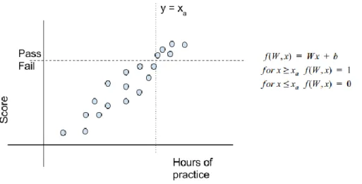
To develop an algorithmic system to classify images there needs to be a mathematical way to discern between different values relevant to some classification criteria. Early attempts at this problem were rule based edge detection, but today's machine learning data based approaches are simpler to write, iterate and they perform much better. Linear classifiers take an input vector, typically containing features in machine learning problems, and transform the values to output a classification decision. The Figure 2 below is example of a binary linear classifier based on the plot where the feature of hours of practice maps to location on the positive or negative side of the pass/fail plane along the score range. A binary linear classifier at y = xaseparates the input values,

assuming data is from well-run experiment one could test the hypothesis that spending greater than xa hours of practice leads to a passing score.

Any series of weights which are combined in linear fashion can be considered a linear classifier. While low dimensional cases are easy to visualize, often machine learning problems have many dimensions as features or more. Linear classifiers are useful because after model training, the classification function is set of linear operations that are computationally cheap.

The weights in the above example could be represented or transformed with many types of functions, initial selection of the appropriate functions takes intuition with the dataset. One of the primary goals in deep learning, or any machine learning, is that algorithms need a good set of weights with right bias to produce meaningful results. Most deep learning algorithms choose a semi-random set of weights and iterate to a state of lower error.

L

OSS

F

UNCTION

The type of weights for a classification problem are coupled with the decision of which type of loss function is used to converge to a solution. This framework for loss function is important because not all problems are straightforward and have geometric intuition like the example of pass/fail. Consider an example where there are other features other than hours of practice for student pass/fail classification. Suppose there is data on age, gender, height, weight, name, student identification number, hair color, previous test scores, grade point average, etc. With some intuition, one could hypothesize that gender, weight, name, and hair color is not a

contributing factor but it would be much harder to hypothesize an accurate weight to previous test score or grade point average.

A loss function helps in deciding what weight values to give a feature vector. For example, in a linear regression problem, one can define the loss as squared loss from the expectation.

SquareLoss(p,y) = (p - y)2 _{where p is the predicted values and y is the actual value}

For example, if the prediction and actual value has delta of less than 1 then there is not a large penalty in the loss function, but as you increase linearly to 1, 2, 3...x then the loss value in the squared loss will greatly increase. In parametric image selection problems or more generalized optimization problems, the goal of the optimization algorithms is to usually minimize the loss

function through iterative steps. The number of parameters might be equal to the number of features so errors can quickly add up. Different types of problems usually have different loss function based on which parameters are important, structure of data and goal of the optimization. For many linear regression problems, the mean squared error serves as effective loss function.

For ANNs which solve image classification problems, one popular method is the cross-entropy loss function. Cross entropy is a concept from information theory [14], involves the Kullback-Leibler divergence, which measures loss between the two probability distributions. For image classification problems, the two distributions are the predicted label and the ground truth label. Softmax classifiers which use cross-entropy loss function can be summarized as the following:

The Softmax cross entropy loss function is popular because ANNs use Softmax functions for their neuron network layers [15][16], a concept covered later in this section

R

EGULARIZATION

When solving real world problems, it is essential to keep models simple so they do not overfit the data. Increasing the complexity is tempting for better results, however, it is better to be more robust than accurate. If the loss function only cares about minimization of error, then there is no incentive to reduce model complexity. For machine learning problems, there are many methods to make simpler model including L1, L2, elastic net, hinge loss, etc. Each technique deals with a different weakness of model behavior in optimization problems. L1 normalization penalizes additional features weights, and tends to promote a few strong features which predict behavior. For problems that have sparse features, L1 can be a useful method. For deep learning problems dropouts, which are covered later in this section, are useful method for regularization.

S

TOCHASTIC

G

RADIENT

D

ESCENT

No discussion of deep learning can be complete without the ever present and useful method of Stochastic Gradient Descent (SGD). The central idea is to iterate and minimize the loss function

through small steps in the direction of minimum loss. Imagine a ball on the top of a hill, in a dynamically unstable position, the direction of least gravitational potential energy for the ball would be down the hill to some lower elevation. If a small force was the ball in all directions, then its potential energy was measured and then the gradient vector of least energy would point to a path down the hill. That’s what a SGD algorithm does, small steps towards a point of

minimization for convex problems. For convex optimization problems, there is an assumption that local minimums equal global minimum, the set is convex and minimum is unique. Many real-world problems are nonlinear and non-convex but useful engineering assumptions can turn many difficult problems into convex problems. SGD has enough popularity to be regarded as a subfield within the optimization literature. Many problems outside of deep learning benefit can loss function minimization through SGD.

Gradient descent algorithm can be defined as algorithms which minimizes from some initial θ value. The α is the learning rate, or how large of a step to take for each update of the algorithm.

J(θ) is the loss function or sometimes termed cost function, the difference is that usually cost functions has a regularization competent.

After some derivation [17], the above formulation can be described as Least Mean Squares rule:

The above equation works for a single training example, repeat the step until convergence. Show below is the algorithm form of the least mean squares rule.

Figure 3: Graph depicting the convergence of SGD algorithm to solution [17]

For a convex function, shown above, the ellipses are the contour of a quadratic function. The blue path starts from an initialized value, and takes incremental steps towards the minimum. Note how each step size in magnitude becomes smaller as convergences gets close; this is because the gradient is getting smaller. Sometimes it can be useful to quicken the pace, to take larger magnitude step if each step is in the same unit vector. SGD with momentum is one of the common optimization methods built on top of a SGD algorithm, the idea is to add additional force to the ball as it rolls down the hill so that it does not explore small local ravines probably do not contain the minimum. Adding larger momentum force can lead to an unstable path which fails to converge, but for many cases tradeoff of faster convergence with less oscillation is worthwhile.

Learning rates, when conservatively chosen, are small and fixed at the start to guarantee convergence because a learning rate which is too large will miss the minimum. The pitfall of choosing a learning rate too small is model cost of runtime will exceed acceptable levels. Nesterov accelerated gradient is another way to give momentum but avoid over indexing on the

latest change, the idea here is to take a leap of faith in the previous accumulated gradient but then make a small correction [18].

An adaptive learning rate algorithm like SGD with momentum, Adagrad, Adadelta, RMSProp, and Adam are popular with ANNs researchers. Adagrad [19] and Adadelta scale model

parameters are inversely proportional to the square root sum of previous values. RMSProp [20] keeps a moving average of the square of the gradients, and is another variation of Adagrad. Adam [21] and its variant Nadam is yet another adaptive learning rate, it has decay of past squared gradients like Ada, but also additional feature of decaying with the average of past gradients. Most deep learning frameworks choose an adaptive leave learning rates algorithm set at some default rate. In the survey of the literature, there is no consensus of which is the optimal learning rate algorithm, most researchers seem to choose whichever algorithm they have familiarity in tuning [22].

Another consideration is the hyperparameter optimization for all these parameters but the practice of such methods is outside the scope of this report since current commodity hardware does not support efficient grid search of hyperparameters for deep learning. There is a whole subfield of SGD optimization which contain many more bags of tricks. Many of them apply to deep learning but each comes with tradeoffs such as increase in performance might increase complexity or might not scale to other datasets. The methods presented in this report are the popular today, but the fast-evolving nature of this field might adopt some other set of SGD optimizations methods.

These parameters settings matter greatly when scaling deep learning networks because

parameters must be shared in some manner in parallel or distributed systems. SGD parallelizes well since it is easy to make the iterative processor a parallel effort with each parallel node responsible to process a small amount of data then synchronizing the parameters at the end of each step. Distributed SGD presents novel challenges, and solving the problem will allow the deep learning technology to move up the TRL scale.

N

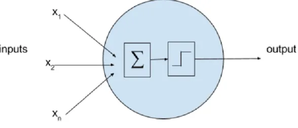
EURON MODEL

In neuroscience, there are still many mysteries of how exactly a biological neuron functions, but there is enough insight from that field to inspire ANNs. A simplified biological model can be described as a black box where inputs are given and the neuron after some computational process either chooses to output a signal or not. Threshold Logic Unit is an abstract model which

represents the function of neuron as shown in Figure 4 below.

Figure 4: Simplified biological neuron model

For a vector of inputs, synapses from other neurons, feed into a neuron where they are processed. There is a nonlinear activation function which allows the signal to pass to other neurons or terminate the signal. Each weight from xt to xn may or not be used in the model, or treated

differently depending on their magnitude. ANNs can be imagined like a human brain, which contains billions of neurons, which means hand tuning is impartial for the conventional programmer. From an engineer’s perspective, the internal tuning of each weight should be an algorithmic and more care must be taken in selection of the types of functions, depth, and architecture used to make each part of the ANNs. From an electrical engineering perspective, neurons in a network are similar to the behavior of logic gates like NAND, NOT, or XOR, etc.

S

OFTMAX FUNCTION

Previously, there was discussion of binary classification problem of pass/fail, but many problems have outputs of varying gradients. For example, consider the classification problem for

handwritten digits, here are 10 distinct values for any given input of a digit image. Instead of running classification algorithm 10 times, one can compute probability for each digit in one output whose sum equals to one. This allows a logistic regression of sorts between layers of the ANNs, and creates a useful probability distribution. The Softmax function is essential for creating layers with depth, to achieve the deep part of deep learning.

F

ORWARD

/B

ACKWARD PROPAGATION

In neural networks which contain many layers and connections the computational time starts to exponentially increase. Ordinarily, there is forward propagating of some gradient computation through the network and on the back end one applies the chain rule to compute the loss function relative to the inputs. Taking a graph model approach, the computation traverses different nodes, each with their own set of weights, with some value across the network, each step usually goes to different layer in the network. The weight constants for each node updates after each traversal, this way the relevant parts of the network can update their weights without expensive methods which globally update the network with a new set of weights for each node.

D

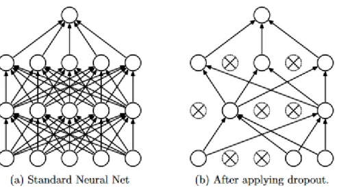
ROPOUTS

Greater depth in network layers for ANNs minimizes loss, but can easily lead to overfitting. Dropouts is a technique where random or semi-random parts of the network are removed during the training process in each iteration to reduce over-fitting like L1 regularization. Dropouts reduce over-fitting and reduce model error but model training can be 2-3 times long for similar architectures [23]. Figure 5 shows a thinner networks post dropout neural net where the path of computation across the graph has less steps and therefore, less computational cost.

Figure 5: Comparison of Standard Neural Net before and after applying dropout [23]

A

CTIVATION FUNCTION

Inside of each neuron after weights have been calculated from each weight, usually through a linear combination, the threshold is either or not met for the value to pass to the next layer. The activation function selection has far reaching impact on performance of the neural network. Popular activation functions include sigmoid, hyperbolic tan (tanh) and Rectified Linear Units (ReLU)

Figure 6: Sigmoid function

σ

(

x

)=1/(1+

e

−x

_{) with a range between 0 and 1}

Sigmoid function is a monotonic S-shaped curve that varies between [0,1]. The ascent of the values from 0 to 1 is steep, similar to other activation functions. The simplicity of the function

makes it a good candidate for neural networks, in fact one can make neural networks based solely on sigmoid functions. Although sigmoids work, in practice other activation functions can

outperform sigmoids. Over time the sigmoid network will saturate to the poles of the functions, so sigmoids will average 0 which leads to a vanishing gradient problem.

Figure 7: Tanh function tanh(x) with a range between -1 and 1

Tanh function varies monotonically from [-1,1] which mean negative values can be encoded into the network unlike sigmoids. For natural problems where words like “not” have a negative effect on sentence structure and meaning it can be useful to capture such information at the neuron level with the tanh function. The zero-centered nature of functions is advantageous but still suffers from vanishing gradients at saturation.

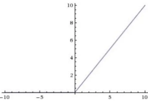
Figure 8: ReLU function which activates when x>0 and responds with linear function

ReLU is probably the most analogous of biological neuron models. When strong signals are allowed to be amplified through the network, there is quicker propagation of information leads to faster convergence. Compared to tanh() or exp() function, ReLU is computation cheaper on the hardware which leads faster iterations. There many variations on ReLU, and it remains the popular method in practice.

M

AX

P

OOLING

,

SHARED WEIGHTS

,

LOCAL RECEPTIVE FIELDS

Local receptive fields means the process of mapping multiple input pixels of an image into a hidden neuron, typically there is reduction in size. In the neuron model these would be the (x1, x2,

x3...) that map to a neuron with some weights and an activation function. Neurons share weights

when useful features have been detected. For example, if there is an edge detection, then that information is shared with the neighbor neurons. This way, if there is another image in the future which is the same classification but rotated in some manner the neural network will quickly converge because the shared weights are invariant to rotations. Max-pooling units are pooling layers inside of convolutional neural networks which extract features from a convolutional layer into a condensed form. Each feature gets a map with relative locations dense with useful

information from the convolution layer. This down sampling operates across the image, is translation invariant and an effective way to reduce dimensionality of the image.

N

EURAL

N

ETWORK ARCHITECTURES

ANNs even with a single hidden layer can approximate any known function. The universality of the neural network means complex hierarchical behaviors can be encoded into the network. For deep learning, there is theoretical importance placed on the depth of the network since

experimentally there is a benefit to deeper networks. Figure 9 below highlights the complex and abundant relationships that occur even when a few layers are used in deep learning. An overly large network will lead to overfitting, that's where dropouts, pruning and other methods are full to manage the network. A too small network will not capture enough system behavior to outperform older machine learning algorithms like support vector machines. Activation functions, SGD optimizations, regularization, initializations and other parameters play an important role in the neural network.

Figure 9: Theoretical relationships between different layers of neural network [34]

C

ONVOLUTIONAL

N

EURAL

N

ETWORKS

By combing all ideas presented in the report thus far, the theoretical underpinnings of a neural network for image classification can be understood. Since images have spatial relations which are important, like edges of sidewalk which denote the drivable road boundary. Yann LeCun in 1998 [24] with the MNIST handwritten digit data set showed how to build Convolutional Neural Networks (CNNs) which combine the ideas of local receptive fields, max pooling, and shared weights.

Figure 10: Convolutional Neural Network architecture Lenet 5 for MNIST dataset [24]

Lenet5 by Yann LeCun shown in the Figure 10 above, maps pixel values from an original input maps all the way to the output with layers of convolution in between. Each layer automatically learns from the preceding layer. For character recognition problems, LeCun demonstrates automated learning for feature extraction outperforms hand crafted algorithms.

In 2012, Alex Krizhevsky created AlexNet [25] which emerged to beat LeNet with use of ReLU, dropouts, max pooling, and advanced GPU hardware to speed up training. This was the start of the popularity of CNNs for image classification competitions in the current AI summer.

Figure 11: AlexNet Architecture [25]

Since 2012, there have been many novel deep learning models like Christian Szegedy’s GoogleNet which reduced computational burden for deep learning with efficient network structure, batch normalization, and other tradeoffs detailed in their research. [26][27]

Figure 12: ResNet’s network-in-network feature [28]

By 2016 new ideas emerged, ResNet [28] is an elegant neural network with the novel idea of adding the output to the next two convolutional layers. This reduced the model size but created much deeper networks, up to 1000 layers deep, that could be trained with micro-architectures features sometimes termed “network”. Figure 12 above shows a typical network-in-network feature in ResNet.

The field is rapidly advancing and there is more work to find useful neural network architectures. In the near future, there might be other ways to layer the network, new activation functions or complex networks-in-networks. Whichever direction the field takes, there needs to be an easy, scalable way to create experiments and deploy in production environments on inexpensive hardware.

The case for parallel computation is easy to make for deep learning, add more cores and

bandwidth and test wider and deeper networks. Since each step is the same from a computational perspective and does not require high precision, even 16-bit half precision floating-point format has shown impressive results. GPUs became popular this decade when NVIDIA, with its CUDA platform, allowed for fast matrix computations with greater performance than a general-purpose CPU. Deep learning can benefit from other hardware architectures like FPGAs or custom ASICS but GPUs have remained the most popular computing architecture to train and test models [29].

GPUs allow for massive parallel operations, and a few GPUs can be put on the same board with a high-speed bus but the energy consumption and cost of these boards can be cost prohibitive. The cost of exotic hardware like NVIDIA DGX-1 which offers high performance computing for $130,000 allows for quick training of model while using 3200 watts of power. The power consumption alone makes such computing a feasible option for firms with large budgets. A truly distributed SGD with asynchronous updates would solve many problems and make deep learning move up on the TRL scale.

D

OWNPOUR

SGD

In 2012 DistBelief [12], published from Google, was one of the early efforts scaling deep learning on a commercial production platform. They tested two main algorithms, L-BFGS and Downpour SGD, for parallel distributed deep learning. Downpour SGD has a mini-batch approach where each server keeps a subset of data, a global model of data and asynchronously updates to a centralized parameter server. Main advantage of an asynchronous model is that experiments are robust to single machine failures, this type of stateless computing is well suited for modern cluster computing on the cloud. In the end, to their surprise, asynchronous Downpour SGD performed better than other methods with the Adagrad learning rate. Previously, Adagrad was not considered as a candidate for nonconvex problems, especially on non-linear deep neural network layers.

Downpour SGD model, shown above in Figure 13, illustrates the centralized parameter server that coordinates between mini-batches of data on each client.

D

ELAY

C

OMPENSATION

SGD

In late 2016 [13] , another model for distributed deep learning emerged from Zheng at Microsoft, where results showed better performance than a synchronous/asynchronous SGD and near parity with a sequential SGD. Here each worker, or client, sends information to a global model to update parameters but afterwards sends a delayed gradient containing an efficient approximation which maybe be useful for the global model as shown in Figure 14. The idea, termed Delay Compensated SGD (DC-SGD), was released under the Microsoft Cognitive Toolkit (CNTK) framework which is a competitor to the many deep learning frameworks currently available in the open source community.

Figure 14: Relationship between workers and Global model [13]

T

ENSOR

F

LOW

In order to investigate how to scale deep learning networks, a trade study was conducted to first choose a framework which would further provide tools for exploration. During the trade study many framework were reviewed including: Theano, Caffe, PyTorch, H20, TensorFlow, and CNTK. The finalist were TensorFlow and CNTK because of the support from the open source community, integration into modern system for ease of deployment, and well cited research papers which demonstrated use of the platform for deep learning research. Eventually

TensorFlow was chosen but the field has not chosen a consolidated platform since it is still in mid-TRL stages. The frequent feature updates to TensorFlow was a deciding factor, every month there have been substantial features additions compared to the other platforms. In the future, most deep learning applications for commercial system might move to TensorFlow at the current rate in the growth of popularity. Of course, the history of computer science is filled with frameworks or languages that seem omnipresent during their hype cycle; only to lose their momentum in a few years and be relegated to niche set of users.

TensorFlow [30], initially released in late 2015, is an open source version of DistBelief which used Downpour SGD for distributed deep learning. The second-generation deep learning framework had input of many more engineers and ran on many hardware platforms including GPUs. Google also created a custom ASIC to optimize TensorFlow training termed tensor processing unit (TPU), which offers numerous cloud services based on TensorFlow and continues to support the framework.

The architecture for TensorFlow is implemented with distributed deep learning from the start, since many of the first users were internal Google users who needed to solve problems across many servers distributed around the globe. Competing frameworks like Theano [31] still do not have distributed support. Other competing frameworks have 3rd _{party support or some minimally}

viable support of distributed capability but these features are as extensive or flexible as TensorFlow. Even though large architectural decisions have already been made for the framework, there is lot of low level exposure to the end users to allow for various software system or hardware optimizations. The core runtime is a cross platform library which sits above a C API detailed in the Figure 15 below:

Figure 15: TensorFlow hardware and software stack [30]

The Delay Compensated SGD and Downpour SGD implemented for report were implemented in Python, results might have differed if this experiment was replicated at the C API level. The distributed master is a scheduler that queues graphs linked computations of the primary data structures. To perform distributed computing, first a user spins up a cluster of nodes which can perform computations on a client-server relationship over the network. The job scheduler can be left to default or directed to give tasks to specific worker nodes in the network. Each node in the distributed cluster operates asynchronously and does not need to communicate with other workers unless directed. Currently, most implementation direct all information to centralized parameter server, similar to Downpour SGD, but in the future, there might be more decentralized parameter servers. The framework supports both model parallelism, where the model is split across clients, and data parallelism where the data is split among clients. Most users favor a mini-batch approach where each node has portion of data local to the client. For deep learning architecture, there is an added benefit of batch normalization to each mini-batch for regularization and accelerates convergence.

To deploy in modern production systems, TensorFlow works well with Kubernets to deploy a cluster of hosts and services on the cloud to quickly scale deep learning as needed. Google,

Amazon, and Microsoft offer cloud computing which integrates well with the TensorFlow framework. Since the hardware is often disintermediated for programmers, it is important to build cross platform system which are agnostic to hardware and do not always rely on the latest

hardware optimizations. Performance must be cost competitive and code should be written in a manner where it can be deployed on another cloud provider. For real world problems, the pipeline for data matters greatly. For now, TensorFlow API integrates with Hadoop HDFS has some support for other filesystems. Other projects like the cluster computing platform Apache Spark have integrated TensorFlow to spin up cluster, hyperparameter tuning, and manage distributed network of nodes. In the future, if the current level of interest holds, TensorFlow may emerge as the dominant deep learning framework across platforms with rich third-party support.

Experiment

To understand the architecture and performance of distributed deep learning systems, the TensorFlow frameworks was chosen for investigation. The two main reasons for TensorFlow framework is the distributed TensorFlow client-server model which allowed for asynchronous execution between nodes, and the ease of which a customized cluster can be initialized. The two algorithms for scaling deep learning were Downpour SGD and Delay Compensated SGD. The asynchronous SGD algorithms were implemented in Python 3.5 on machines which compiled the latest TensorFlow r1.2 master release from GitHub source. By default the Downpour SGD implementation is present in TensorFlow, and Delay Compensated implementation was written for this report.

In order to set up a distributed system, worker nodes and a parameter server is initialized across the available computing resources. After the code was written, the Python scripts were patched with source code to create a Kubernet container image for easy deployment. Each Kubernet instance starts a TensorFlow session which creates a local server on the machine. Each session object holds the all the cluster specifications with addresses over TCP/IP protocol to all other distributed nodes. Each node can be assigned unique names, be part of groups or partition computing resources. There can be multiple sessions per node, and it is possible to have parameter server and worker sessions assigned to same node. Each session object can execute operations from different jobs, however, for this experiment only one job was started so that all available computing resources could be allocated to test Downpour and Delay Compensated SGD.

The ANNs for this experiment on MNIST dataset was a deep neural network with 3 layers. The first two layer had 64 nodes with tanh activation function, L2 regularizer, and dropouts. The final layer had Softmax layer with 10 nodes for the output classification for the digit values. The optimizer was Downpour SGD or Delay Compensation with cross entropy for loss function. Each model was run for 20 epochs with 55,000 iterations per epoch.

To scale deep learning networks, it is crucial to have distributed deep learning on commodity hardware. Most firms rent computing power from one of the main cloud providers, and pay by the minute per transaction over the network and computing power. For distributed model training, GPUs are popular for deep learning but come at a steep cost. Table 1 below shows how much the price difference varies for over a year of operation on the Google Cloud with August 2017 pricing data. The price estimation assumes an Ubuntu operating system, local SSD of 375 GB per

machine, and does not account for the cost of persistent disk storage, load balancing or other network costs. [32]

Computer Type /

number of instances Total vCPUs Total RAM

Total number of K80 GPUs Total VRAM Cost per year ($ USD) N1-standard-1 / 4 4 15 0 0 1,272.17 N1-standard-8 / 4 32 120 0 0 12,244.24 N1-highmem-16 / 4 64 416 0 0 27,156.53 N1-standard-1 / 1 1 3.75 1 24 4,598.06 N1-standard-8 / 1 8 30 4 96 20,595.77 N1-highmem-16 / 1 16 104 8 192 41,410.21

Table 1: Google Cloud pricing for computing instances

Nvidia K80 GPUs offer performance but come at a steep scaling cost when compared to cheaper and less computationally powerful CPUs. Nvidia also offers CUDA framework which allows programmers to access high performance computing for GPUs [33]. There are valid reasons to optimize for GPUs but most traditional computing has been performed with commodity CPU clusters and not high performance GPU clusters. For firms with modest resources, in order to move up the TRL scale, the option which is most cost effective tends to be chosen rather than best conceivable system for model training. Commercial applicants prefer distributed systems because it is cheaper to scale up or down with demand, and customers tend to be located globally so investing high amount of resources in one centralized server with exotic performance does not fit well with their model of worldwide operations.

For this experiment to test scaling of deep learning networks, TensorFlow was deployed on Google Cloud compute n1-standard-4 machines with 20 GB SSD, Ubuntu 16.04 LTS, 15 GB RAM per machine, with a virtual quadcore Intel Skylake processors or later. In terms of

performance, compiling software from source code or using Kubernetes container image did not affect the results. This has important commercial implications because modern developer operation practices favor fast spin up of instances to meet high demand.

Different configuration of hyperparameters were tested 20 times for 4, 8, and 12 nodes. Each additional node configured with the same settings and in the same regional network. One arbitrary server was chosen as parameter server the rest of the nodes operated as workers in an asynchronous manner.

Figure 16: Downpour SGD vs DC-SGD for a typical epoch

Figure 16 shows typical training results for Deep Neural Network for MNIST dataset using Downpour SGD and Delay Compensated SGD. Note how there is stability of performance per epoch within milliseconds for both methods.

Number of nodes Downpour SGD

(average epoch time in seconds)

Delay Compensated SGD (average epoch time in seconds)

4 3.52 3.59

8 3.53 3.61

12 3.55 3.64

Table 2: Average run time per node

The performance of Delay Compensated-SGD has parity, the data shows that it takes a few milliseconds longer but this is probably attributed to the extra communication overhead for Delay Compensated SGD. Table 2 shows how increases in the number of nodes from 4 to 12 for

Downpour increases epoch time by 0.03 seconds and Delay Compensation by 0.05 seconds. This delta of time results in 0.8% increase for Downpour and 1.4% for Delay Compensated. This implies that increase of nodes from 4 to 12 will incur about a 1% on performance in either distributed protocol. Changes to activation functions, number of layers, dropouts, learning rate and loss functions do change behavior in a neural network. For this experiment those parameters were kept constant between runs, but a typical environment will have variable parameters depending on project requirements. Another consideration is the depth of the neural network, network-in-network features, size of data which cause data disk access latency, and higher precision requirements have larger effects than Downpour SGD vs Delay Compensated SGD when all factors are kept constant.

Conclusion

Scaling deep learning remains an important issue to solve for image processing and other related AI problems. Many parts of deep learning components including algorithms, software systems, hardware and data are needed to improve and elevate deep learning to the higher TRL stages. Although GPUs promise superior performance, it will likely remain an option for well-resourced firms. For asynchronous Downpour SGD or Delay Compensated SGD which offer cost effective CPU deep learning, there is room for improvement. In the future, perhaps custom ASICs like TPU might dominate deep learning, but even then the TPUs will need some asynchronous protocol for communication between nodes in the cluster.

From a software engineering perspective, it is important to build a robust system which can tolerate failure of any one node. This report shows that asynchronous Downpour SGD or Delay Compensation SGD offers effective distributed protocol for high performance cluster computing to solve deep learning problems. The total error and model training runtime depends on many factors not covered in this report, but the concern for distributed computing plays an important role in commodifying deep learning technologies.

During the prototype phase for this report, the algorithms were tested in virtual environments on a local desktop machine. The prototype code migrated well to the experimental apparatus in the Google Cloud. This implies is that further research can be conducted on local machines before deploying to costly hardware. Future work could include testing more complex network architectures with network-in-network features or larger datasets. Another interesting

investigation is to have multiple parameter servers which coordinate hyperparameters between them for an effective grid search of hyperparameters. For commercial applications, distributed databases like Apache Hadoop is an important competent in commercial technology stacks where data for a project can come from many sources with varying fidelity. Most researchers use well labeled static datasets, but distributed model training on noisy streaming data from uncertain sources would be challenging. As of 2017, it is hard to know how much longer this current AI summer will last but for the time being, there are many avenues for fruitful research.

Appendix

NASA Technology Readiness Level (TRL)

Technology readiness level Description

1. Basic principles observed and reported

This is the lowest "level" of technology maturation. At this level, scientific research begins to be translated into applied research and development.

2. Technology concept and/or application formulated

Once basic physical principles are observed, then at the next level of maturation, practical applications of those characteristics can be 'invented' or identified. At this level, the application is still speculative: there is not experimental proof or detailed analysis to support the conjecture.

3. Analytical and

experimental critical function and/or characteristic proof of concept

At this step in the maturation process, active research and development (R&D) is initiated. This must include both analytical studies to set the technology into an appropriate context and laboratory-based studies to physically validate that the analytical predictions are correct. These studies and experiments should constitute "proof-of-concept" validation of the applications/concepts formulated at TRL 2. 4. Component and/or

breadboard validation in laboratory environment

Following successful "proof-of-concept" work, basic technological elements must be integrated to establish that the "pieces" will work together to achieve concept-enabling levels of performance for a component and/or breadboard. This validation must be devised to support the concept that was formulated earlier, and should also be consistent with the requirements of potential system applications. The validation is "low-fidelity" compared to the eventual system: it could be composed of ad hoc discrete components in a laboratory.

5. Component and/or breadboard validation in relevant environment

At this level, the fidelity of the component and/or breadboard being tested has to increase significantly. The basic technological elements must be integrated with reasonably realistic supporting elements so that the total applications (component-level, sub-system level, or system-level) can be tested in a 'simulated' or somewhat realistic environment.

6. System/subsystem model or prototype demonstration in a relevant environment (ground or space)

A major step in the level of fidelity of the technology demonstration follows the completion of TRL 5. At TRL 6, a representative model or prototype system or system - which would go well beyond ad hoc, 'patch-cord' or discrete component level breadboarding - would be tested in a relevant environment. At this level, if the only 'relevant environment' is the environment of space, then the model/prototype must be demonstrated in space.

7. System prototype demonstration in a space environment

TRL 7 is a significant step beyond TRL 6, requiring an actual system prototype demonstration in a space environment. The prototype should be near or at the scale of the planned operational system and the demonstration must take place in space.

8. Actual system completed and 'flight qualified' through test and demonstration (ground or space)

In almost all cases, this level is the end of true 'system development' for most technology elements. This might include integration of new technology into an existing system.

9. Actual system 'flight proven' through successful mission operations

In almost all cases, the end of last 'bug fixing' aspects of true 'system development'. This might include integration of new technology into an existing system. This TRL does not include planned product improvement of ongoing or reusable systems.

References

[1] N. J. Nilsson, "THE QUEST FOR ARTIFICIAL INTELLIGENCE, A HISTORY

OF IDEAS AND ACHIEVEMENTS," 08 2017. [Online]. Available:

https://ai.stanford.edu/~nilsson/QAI/qai.pdf.

[2] G. E. Hinton, N. Srivastava, A.

Krizhevsky

, I. Sutskever and R. R. Salakhutdinov,

"Improving neural networks by preventing co-adaptation of feature detectors," 07

2012. [Online]. Available: https://arxiv.org/abs/1207.0580.

[3] "CIFAR-10 dataset," University of Toronto, [Online]. Available:

https://www.cs.toronto.edu/~kriz/cifar.html. [Accessed 01 08 2017].

[4] "Advances in Neural Information Processing Systems (NIPS) 23," 2010. [Online].

Available:

https://papers.nips.cc/book/advances-in-neural-information-processing-systems-23-2010.

[5] B. Graham, "Fractional Max-Pooling," 12 05 2015. [Online]. Available:

https://arxiv.org/abs/1412.6071. [Accessed 08 2017].

[6] S. Thrun, "Stanley: The Robot that Won the DARPA Grand Challenge,"

Journal of

Field Robotics,

vol. 23, no. 9, p. 661

–

692, 2006.

[7] Mobileye, "The Evolution of EyeQ," [Online]. Available:

http://www.mobileye.com/our-technology/evolution-eyeq-chip/. [Accessed 01 08

2017].

[8] Tesla, "Software Updates," [Online]. Available: https://www.tesla.com/software.

[Accessed 10 08 2017].

[9] S. International, "Taxonomy and Definitions for Terms Related to Driving

Automation Systems for On-Road Motor Vehicles," 30 09 2016. [Online].

Available: http://standards.sae.org/j3016_201609/. [Accessed 01 08 2018].

[10] E. Musk, "Master Plan, Part Deux," Tesla, 20 07 2016. [Online]. Available:

https://www.tesla.com/blog/master-plan-part-deux. [Accessed 01 08 2017].

[11] D. Silver, "Mastering the game of Go with deep neural networks and tree search,"

Nature,

vol. 529, pp. 484-489, 2016.

[12] G. S. C. R. M. K. C. M. D. Q. V. L. M. Z. M. M. R. S. P. T. K. Y. A. Y. N. Jeffrey

Dean, "Large Scale Distributed Deep Networks," 2012. [Online]. Available:

https://static.googleusercontent.com/media/research.google.com/en//archive/large_

deep_networks_nips2012.pdf. [Accessed 01 08 2017].

[13] Q. M. T. W. W. C. N. Y. Z.-M. M. T.-Y. L. Shuxin Zheng, "Asynchronous

Stochastic Gradient Descent with Delay Compensation," 14 07 2017. [Online].

Available: https://arxiv.org/abs/1609.08326. [Accessed 01 08 2017].

[14] J. A. T. Thomas M. Cover, Elements of Information Theory, 2nd Edition, Wiley,

2006.

[15] Stanford, "CS231n Convolutional Neural Networks for Visual Recognition,"

[Online]. Available: http://cs231n.github.io/neural-networks-2/. [Accessed 01 08

2017].

[16] L. L. a. H. Qi, "Learning Effective Binary Descriptors via Cross Entropy,"

2017

IEEE Winter Conference on Applications of Computer Vision (WACV),

pp.

1251-1258, 2017.

[17] A. Ng, "CS229 Lecture notes," [Online]. Available:

http://cs229.stanford.edu/notes/cs229-notes1.pdf. [Accessed 01 08 2017].

[18] G. Hinton, "Neural Networks for Machine Learning, CSC321," [Online].

Available:

http://www.cs.toronto.edu/~tijmen/csc321/slides/lecture_slides_lec6.pdf.

[Accessed 01 08 2017].

[19] E. H. Y. S. John Duchi, "Adaptive Subgradient Methods for Online Learning and

Stochastic Optimization,"

Journal of Machine Learning Research,

vol. 12, pp.

2121-2159, 2011.

[20] G. H. T. Tieleman, "Neural Networks for Machine Learning, Lecture 6.5,"

COURSERA, 2012.

[21] J. B. A. D. Kingma, "A method for stochastic optimization," International

Conference on Learning Representations (ICLR), 2015.

[22] I. G. a. Y. B. a. A. Courville, Deep Learning, MIT Press, 2016.

[23] G. H. A. K. I. S. R. S. Nitish Srivastava, "Dropout: A Simple Way to Prevent

Neural Networks from Overfitting,"

Journal of Machine Learning Research 1,

vol.

15, pp. 1929-1958, 2014.

[24] L. B. Y. B. P. H. Yann LeCun, "Gradient-Based Learning Applied to Document

Recognition,"

Proceedings of IEEE,

vol. 86, no. 11, pp. 2279-2324, 1998.

[25] I. S. G. E. H. Alex Krizhevsky, "ImageNet Classification with Deep Convolutional

Neural Networks,"

Advances in Neural Information Processing Systems 25,

2012.

[26] W. L. Y. J. P. S. S. R. D. A. D. E. V. V. A. R. Christian Szegedy, "Going Deeper

with Convolutions," 17 09 2014. [Online]. Available:

https://arxiv.org/abs/1409.4842. [Accessed 01 08 2017].

[27] A. P. E. C. Alfredo Canziani, "An Analysis of Deep Neural Network Models for

Practical Applications," 14 04 2017. [Online]. Available:

https://arxiv.org/abs/1605.07678. [Accessed 01 08 2017].

[28] X. Z. S. R. J. S. Kaiming He, "Identity Mappings in Deep Residual Networks," 25

07 2016. [Online]. Available: https://arxiv.org/abs/1603.05027. [Accessed 01 08

2017].

[29] NVIDIA Corporation, "NVIDIA DGX-1," [Online]. Available:

https://www.nvidia.com/en-us/data-center/dgx-1/. [Accessed 01 08 2017].

[30] Google, "TensorFlow: An open-source software library for Machine Intelligence,"

[Online]. Available: https://www.tensorflow.org/. [Accessed 01 08 2017].

[31] "Theano at a Glance," LISA lab, 21 04 2017. [Online]. Available:

http://deeplearning.net/software/theano/introduction.html. [Accessed 01 08 2017].

[32] Google, "Google Cloud Platform Pricing Calculator," [Online]. Available:

https://cloud.google.com/products/calculator/. [Accessed 01 08 2017].

[33] NVIDIA, "CUDA Zone," [Online]. Available:

https://developer.nvidia.com/cuda-zone. [Accessed 01 08 2017].