1
A multiple-point spatially weighted
k
-NN method for
object-based classification
Yunwei Tang1, Linhai Jing1, Hui Li1, Peter M. Atkinson2, 3, 4
1 Key Laboratory of Digital Earth Sciences, Institute of Remote Sensing and Digital Earth, Chinese Academy of Sciences, No. 9 Dengzhuang South Road, Beijing 100094, China
2 Faculty of Science and Technology, Engineering Building, Lancaster University, Lancaster LA1 4YR, UK
3 School of Geography, Archaeology and Palaeoecology, Queen’s University Belfast, Belfast BT7 1NN, Northern Ireland, UK
4 Geography and Environment, University of Southampton, Highfield, Southampton SO17 1BJ, UK
Abstract
Object-based classification, commonly referred to as object-based image analysis (OBIA), is now commonly regarded as able to produce more appealing classification maps, often of greater accuracy, than pixel-based classification and its application is now widespread. Therefore, improvement of OBIA using spatial techniques is of great interest. In this paper, multiple-point statistics (MPS) is proposed for object-based classification enhancement in the form of a new multiple-point k-nearest neighbour (k-NN) classification method (MPk-NN). The proposed method first utilises a training image derived from a pre-classified map to characterise the spatial correlation between multiple points of land cover classes. The MPS borrows spatial structures from other parts of the training image, and then incorporates this spatial information, in the form of multiple-point probabilities, into the k-NN classifier. Two satellite sensor images with a fine spatial resolution were selected to evaluate the new method. One is an IKONOS image of the Beijing urban area and the other is a WorldView-2 image of the Wolong mountainous area, in China. The images were object-based classified using the MPk-NN method and several alternatives, including the k-NN, the geostatistically weighted k-NN, the Bayesian method, the decision tree classifier (DTC), and the support vector machine classifier (SVM). It was demonstrated that the new spatial weighting based on MPS can achieve greater classification accuracy relative to the alternatives and it is, thus, recommended as appropriate for object-based classification.
2
Keywords
Multiple-point statistics, k-NN, object-based classification, training image
1 Introduction
Classification using fine spatial resolution imagery is a widespread goal in remote sensing, and one that is not straightforward to solve with high accuracy (Wang et al., 2013). It is generally agreed that object-based image analysis (OBIA) has several advantages compared to pixel-based analysis for processing fine spatial resolution remotely sensed data (Blaschke and Strobl, 2001; Myint et al., 2011). In object-based classification, segmentation is first applied to images, decomposing the image scene into relatively homogeneous objects (or segments) based on the arrangement of pixel values across the image, which should reflect the set of real-world objects of interest (Newman et al., 2011). Then, instead of classifying based on the spectra of each pixel, classification is undertaken based on the spectral information of each resulting
segment.
Object properties and spatial context are important for OBIA classification in remote sensing. Information on the classes of neighbouring objects can be used to either increase classification accuracy or to identify land use or function that is otherwise challenging. An example of the latter is the ability to identify a railway station from the character of the objects that comprise it (e.g., long thin platforms, long thin roofs) and the set of objects that surround it (e.g., railway lines, car park and multiple roads). Commonly, a spatial weighting is incorporated into the classifier to increase the accuracy of the classification result. Classifiers that use spatial information combined with spectral information are known as contextual classifiers (Jensen, 1979). It has been suggested that such contextual classifiers can reduce noise and achieve greater accuracy than non-contextual classifiers (Park et al., 2003; Pasolli et al., 2014). Geostatistical techniques have been applied to pixel-based classifiers as a contextual classification method (Atkinson and Lewis, 2000), although all the spatial weighting schemes investigated in this case were based on two-point statistics (i.e., the relationship between the central pixel and its neighbours).
Recently, advances in multiple-point statistics (MPS) have shown that two-point statistics are limited. Instead of two-point-based functions such as the variogram, MPS borrows structures from training images, from which higher-order local patterns of the target field can be captured. Thus, spatial structures can potentially be characterised more completely using MPS. Recently, a few studies applied MPS to the classification of remotely sensing data. For example, Boucher (2009) realised super-resolution mapping with MPS. Ge and Bai (2011) extracted linear objects from satellite sensor imagery using MPS. Tang et al. (2013) proposed a post-classification method using MPS and compared it with contextual classification based on the
3
Markov random field model. Nevertheless, MPS for the classification of fine spatial resolution imagery remains under-explored.
Previous studies have demonstrated the advantages of contextual classification and MPS, independently. Thus, the overall aim of this paper, given the popularity and already high accuracies achievable with OBIA and the potential of MPS relative to two-point statistics, is to explore the utility of incorporating an MPS-based spatial weighting into the OBIA approach. Specifically, a new MPS spatial weighting for incorporation into the k-NN method is proposed for object-based classification. The proposed method utilises a training image as prior knowledge to characterise the spatial correlation between multiple points of land cover class, an approach used widely in MPS. The MPS borrows spatial structures from multiple parts of the training image and then incorporates this spatial information, in the form of multiple-point probabilities, into the k-NN classifier. The hypothesis is that a MPS weighting scheme has the potential to increase the accuracy of the k-NN classifier relative to two-point-based spatial weighting schemes. The specific goals of the paper were, therefore: (i) the development of a new MPS spatial weighting for remotely sensed contextual classification, and (ii) evaluation of the applicability of the new method for handling objects (c.f., the previous pixel-based implementation).
2 Methods
2.1 The MPS approach
MPS characterises spatial dependence from a training image, which is required to depict the types of structures that the target image and, thus, the expected realisations should exhibit (Boucher, 2009). A training image substitutes for the variogram or covariance function in traditional geostatistics and provides prior knowledge for spatial correlation modelling. A data template with a central node u is defined as T(u) = {h1, …, hn}, which is composed of n locations ui (i = 1, …, n), where hi is a
distance vector between ui and u. The data template T(u) is used to scan the training
image. To capture multiple-point statistical information, a data event consists of categorical values and is obtained by the same shape of template that is used to scan the training image. A data event can be expressed as dev(u) = {c(u1), …, c(un)}, where
c(ui) (i = 1, …, n) is the categorical value at location ui within the template (Okabe
and Blunt, 2005).
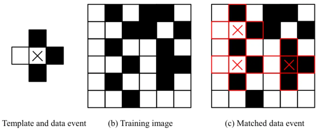
The frequency of a data event can be calculated when the training image is scanned by a template. Figure 1 gives a binary example, in which the cross-shaped data template consists of three black nodes and one white node (Figure 1a), and the central node is unknown. This template is used to scan the training image in Figure 1b. Sixteen data events are extracted, and three matched data events are found in the training image (Figure 1c). As can be seen, two of the three matched data events have
4
a white central node and one has a black central node. Therefore, the frequency with which the data event occurs in the training image is 3/16, and the central node of this data event has a probability of 2/3 to be white and 1/3 to be black.
The multi-grid simulation approach can be adopted in MPS to capture structures of different sizes in the training image (Tran, 1994). The multi-grid approach expands the size of the simulated grid while not increasing the number of nodes. It is assumed that the data template T(u) has L multi-grid levels. The new geometrical template is
constructed by rescaling the original template:
1 1
1
( ) 2 , ,2
L L L
n
T u h h .
2.2 Distance and geostatistically weighted k-NN
In the k-NN method, the classifier allocates pixels to the neighbours to which it is closest in feature space. An inverse distance weighting (IDW) function can be incorporated into the k-NN classifier to give more weight to a neighbour closer to the unclassified observation than to a more distant neighbour (Dudani, 1976). IDW can be expressed as:
uk 1p uk
d
(1) where duk measures the distance between the current pixel u and its neighbouring
training pixel k in feature space, ωuk is the weight based on an inverse distance, and
the exponent p is an integer that determines the magnitude of the weight. The abbreviation wk-NN is used to refer to the IDW-based k-NN.
In the geostatistically weighted k-NN (gk-NN) method, the probability that a pixel u
belongs to class m can be evaluated as follows (Atkinson and Naser, 2010):
, 1 g NN , 1 1 1 1 K g m m uk uk g uk k k M K g m m uk uk g uk m k S p S p c u m S p S
h h (2)where the subscript uk of h indicates the lag between pixel u and its neighbour k. K
refers to the total number of neighbours in feature space. pm m,
huk and pm m,
hukare the fitted models of the spatial cross-covariance, which also refers to the class-conditional probability. Term m' is a class index for m' = 1, …, M classes, and m
is the class of interest. Sg is a proportional weight between 0 and 1. The
class-conditional probability pm m,
huk of a pixel u belonging to class m, given a5
1 , 1 | N i m m uk N i I c m c u m p I c u m
h h (3)where N is the number of training pixels in the image, and c(h) represents the class value at lag h (i.e., the class at the neighbouring pixel location k). The class-conditional probability pm m,
huk can be inferred similarly. The indicatorfunction I takes a value of one if the condition is satisfied, otherwise zero. The spherical, exponential and Gaussian models are usually fitted to the class-conditional probability plot (Armstrong, 1998). The k-NN and gk-NN methods were used in the experiments as benchmark methods, while the wk-NN method was implemented to provide additional information on the proposed method.
2.3 Multiple-point weighted k-NN
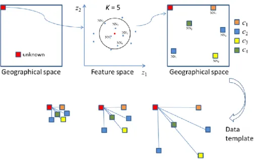
The standard k-NN classifier retains the location information of the K neighbours in feature space and, thus, the geographical weighting is readily integrated into the k-NN classifier. In the MPS-based k-NN approach (MPk-NN), instead of using two-point statistics, the conditional probability representing the spatial information is provided by multiple point analysis of the training image. For an unknown location u, K nearest neighbour training pixels uk can be found. Thus, the data template at location u can be
defined as T(u) = {h1, …, hK}, where hk is the lag between uk and u. So the template
centred at u consists of the same separation lag (for both distance and direction) and classes as the neighbouring K pixels in the prediction data. This template is used to scan the training image and derive the multiple-point probability for pixel u by counting the replicates of the data event dev(u), where dev(u) = {c(u1), …, c(uK)}. The
probability of pixel u with class m equals the proportion of the number of dev(u) that possesses class m at the central node to the total number of dev(u). For a different location, a different template is applied to estimate another probability from the training image. The multiple-point probability of a pixel u belonging to class m is, thus, expressed as:
1 MP 1 | 1 1 N u N u I c u m dev u p c u m I dev u
(4)Note that dev(u) = 1 means that the data event dev(u) is found in the training image, indicating that all the K pixels at location uk should match exactly the corresponding
classes (i.e., c(uk) = mk (k = 1, …, K)). If the multi-grid concept is applied, the
6
1 MP 1 1 | 1 1 1 N l L L u N l l u I c u m dev u p c u m L I dev u
(5)l indicates that a data event is searched at the lth multi-grid level. Here, instead of expanding the data template, the template is rescaled by condensing the original template. A compact data template is more suited to capturing spatial dependence since near things tend to be similar. Also, the template can sometimes be spatially extensive, such that expanding the template may fail to capture data events inside the
training image. Thus, the data template was formed as:
1 1
1
( ) 2 , , 2
L L L
n
T u h h . For example, if L is taken as 3, the data template was
1/2 and 1/4 of the original template for L = 2 and 3, respectively. Figure 2 displays an example of data template construction and the data templates with a multi-grid level of 3. Thus, the multiple-point enhanced k-NN classifier (MPk-NN) can be written as:
MP NN MP MP MP g NN 1 MP 1 1 g , g 1 MP g , g 1 1 1 | 1 1 1 1 1 1 k k N l L u N l l u K m m uk uk uk k M K m m uk uk uk m k p c u m S p c u m S p c u m I c u m dev u S L I dev u S p S S S p S
h h (6)Similar to Sg, SMP is a multiple-point spatial weighting added to the k-NN classifier,
ranging from 0 to 1.
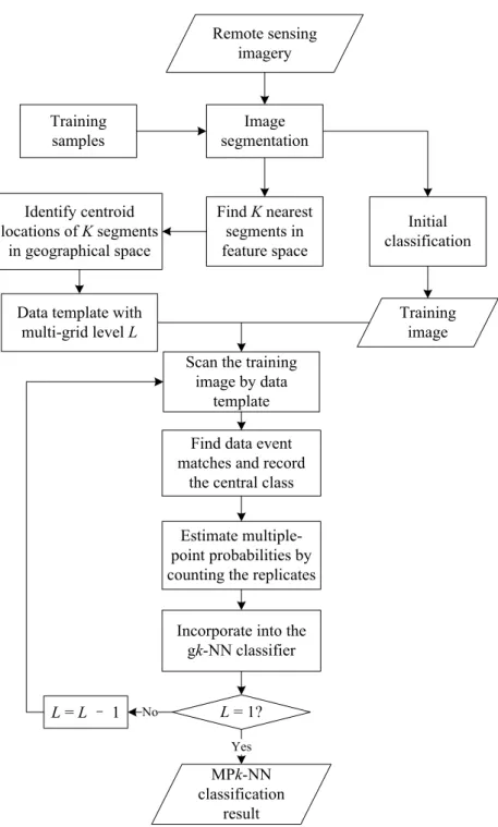
To apply the MPk-NN method for object-based classification, the central point of each segment is first extracted. The central locations are recorded, so that the distance between any two segments can be inferred. Since a pre-classified image of the same area can guarantee a similar spatial distribution of land covers, the training image is derived from an initial classification result. The flowchart of the MPk-NN classification is shown in Figure 3. It should be noted that, here, the k-NNs are segments, and the distances from the current segment to the k-NNs are measures of the relations between the centres of the segments. However, the scanning process is pixel-based, from top to bottom and left to right of the whole training image. The replicates of the data events are recorded according to the class type of the central node. This information is then converted to a conditional probability for each class and incorporated into the gk-NN classifier, as shown in Equation (6).
7
3 Experiments
3.1 Study area
To evaluate the new method, two experiments were defined. The experiments were selected to cover two very different environments, one a highly structured anthropogenic urban environment and the other a relatively untouched natural environment. These different environments were chosen because the land cover-land use (LCLU) objects of interest are quite different spatially, thus, providing a more extensive test of the new approach. In the urban environment, the objects are generally artificial, including a complex and dense arrangement of buildings interwoven with roads, on a vegetated background. In the natural environment, the objects arise as a mosaic of different vegetation types, with the objects themselves having more heterogeneous boundaries compared to the objects in the urban environment.
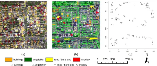
The proposed MPk-NN method was first applied to classify LCLU objects in an urban scene in Beijing, China. Identifying urban objects from fine spatial resolution imagery in urban areas is a common and important objective (Johnson and Xie, 2013). The typical urban area can be classified generally into four high-level classes: buildings, vegetation, road/bare land and shadow. The challenge here is to distinguish the building class from road/bare land. Because these two classes have similar spectral responses, but different spatial distributions their separation is challenging using traditional spectral-only classifiers. For this task, we selected an IKONOS image (39°57ʹ55ʺ–39°58ʹ28ʺN, 116°24ʹ5ʺ–116°24ʹ49ʺE) with a spatial resolution of 4 m and size 256 256 pixels over the Beijing urban area (Figure 4a), acquired in May 2000 (4-band bundle, processing level: standard 2A). This image was chosen because of its fine spatial resolution, but alternatives with a similar spatial resolution would be equally applicable for this experiment.
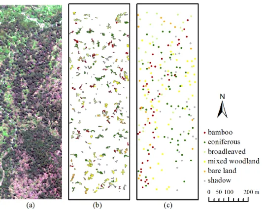
The second experiment was defined at Dengsheng Ditch in Wolong region, Sichuan Province, China (Figure 5a). A few wild giant pandas live in this area and, thus, knowledge of the spatial distribution of bamboo, which is the main source of food for giant pandas, is required as part of identifying suitable habitat for giant pandas. However, the vegetation types in this area are similar spectrally meaning that traditional spectral-only classifiers may struggle to achieve sufficient accuracy. As stated above, it is also of interest to evaluate how the proposed method performs when applied to a natural scene in which the individual objects have heterogeneous boundaries. For this experiment, we chose a WorldView-2 image subscene (30°50ʹ19ʺ–30°50ʹ51ʺN, 102°57ʹ35ʺ–102°57ʹ48ʺE) with a spatial resolution of 2 m and size 493 161 pixels, acquired on 28th May 2014 (8-band bundle, processing level: standard 2A). Again, the image was chosen because of its fine spatial resolution, which was required to resolve the forest patches of interest. The images used in both experiments are processed at the standard 2A level, which means that they are radiometrically corrected, sensor corrected, and a coarse digital elevation model
8
(DEM) is applied in the geometric correction. This product is sufficient to support the experiments in the present case.
3.2 Data pre-processing
Image segmentation was first applied to derive homogeneous objects in the images. Only multispectral bands were used in the following processes. 1348 image objects were delineated in the IKONOS image with a mean size of 48.6 pixels, and 5975 image objects were derived in the WorldView-2 image with a mean size of 13.3 pixels.
Training samples were used for two objectives. One was to train the classifier, and the other was to estimate the class-conditional probability for geostatistical modelling. The environment is complex in Wolong, so the procedure for the selection of training and reference data for experiment II was different to that for experiment I.
Reference data were provided to test the classification result. In the first experiment, the training and reference data were labelled manually by inspection of the image since the four classes in the IKONOS image could be identified readily by visual inspection. The IKONOS product does not require further geometric correction when selecting samples manually. Thus, 276 points were selected as the reference data for validating the classification (Figure 4a), and 35 training sample segments were selected manually from the 1348 possible segments (Figure 4b). These training segments were used to train the k-NN classifier. Although the size of training set (35 segments relative to the total number of 1348) was appropriate for classification, geostatistical modelling requires more sample data. Furthermore, the training segments are not suitable for geostatistical modelling as the model of spatial covariance is a function of lag. Each segment accounts for an area, so the distance measured between segments varies. Therefore, instead of segments, sample points (i.e., pixels) were used for geostatistical modelling. A stratified sampling scheme was applied to the 35 training segments. 50 sample points were selected for each class and, thus, 200 points were selected in total for geostatistical modelling (Figure 4c).
In the second experiment, it was difficult to identify forest cover types directly from the image. Therefore, two field visits were carried out at Dengsheng Ditch, on 13th June 2014 and 12th September 2014. Since the geometric accuracy required is higher in experiment II than in experiment I (where the reference data were chosen directly from the image), the WorldView-2 image required further geometric correction. The first visit aimed to measure feature points for image geometric correction and the collection of training samples, and the second field visit was undertaken to collect reference data.
A Trimble○R
GeoXHTM 6000 handheld GPS with an antenna was used to collect location points in the field. The four forest cover types in the classification are defined as bamboo, coniferous, broadleaved and mixed woodland. Two further categories were included: bare land and shadow. The four types of woodland cover were
9
recorded when collecting sample points in the field. Training samples for the other two classes were chosen manually from the image, since they were easily identified in the WorldView-2 image. In total, 312 sample segments were used for training and 223 sample points were used for testing, which are shown in Figure 5b and 5c, respectively. Here, 312 training samples were sufficient to fit the geostatistical models, so the samples for modelling were the same as those used for classification.
The training image is necessary in MPS to characterise spatial structure, which is provided as prior knowledge to the classification task. In both experiments, the training images were produced from pre-classified images using the wk-NN method.
3.3 Classification
The classification process was the same for both experiments. To test the effectiveness of the proposed method, different benchmark classification methods were applied to compare with the MPk-NN classifier. The k-NN method is based on spectral information only, while the geostatistical weighting is added in the gk-NN method, so these two benchmarks were used to deduce directly the influence of the MPS weighting. The k-NN classifier was first applied based on the mean value of the spectral bands of each segment and with K = 5. For the gk-NN method, class-conditional probability plots were first estimated from the selected sample points for geostatistical modelling and then fitted with covariance-type models. Then the gk-NN method was applied using Equation (2). To provide other benchmarks against which to assess performance, three popular classification methods were applied: the Bayesian, decision tree classifier (DTC) and support vector machine (SVM) methods. The aim was to determine if the MPS-based method can outperform these other state-of-the-art classifiers. Finally, the MPk-NN method was applied. The classification map derived from wk-NN was used as the training image, which itself was not used as a benchmark method. The data template for each pixel consisted of
k-NN nodes (K = 5). The multi-grid level L was taken as 3.
3.4 Results and analysis
The classification results obtained using the above six methods are displayed in Figures 6 and 7 for both experiments. Tables 1 and 2 summarise the accuracies achieved using the six classification methods. The overall accuracy, user’s accuracy, producer’s accuracy, and Kappa coefficient are reported.
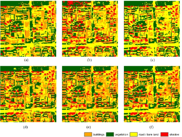
In the first experiment, some shadows were misclassified as buildings in the Bayesian result. The accuracies of the building class are low (around 50%), and the producer’s accuracy (65.96%) of the shadow class was the lowest using the Bayesian method. The accuracies of the vegetation class are rather high (all above 95%) except for the DTC method. The decision tree confused some trees with shadows in the upper left of the image. For the classes of buildings and road/bare land, MPk-NN produced the greatest accuracies, whereas the SVM method produced the lowest accuracies. Most buildings in the SVM result were misclassified. These three methods (Bayesian, DTC,
10
and SVM) produced limited accuracies because only spectral information was used for classification.
The k-NN method, although also based on spectral information only, is more suited to classifying the large segments and, thus, resulted in greater accuracy than the other three methods. The k-NN and gk-NN methods produced the same overall accuracy, but more buildings are shown in the upper right part of the image for the gk-NN and MPk-NN results than for the k-NN result. The buildings increased in coverage using the gk-NN and MPk-NN methods, which was caused by the spatial weightings. The MPk-NN method produced the greatest overall accuracy and Kappa coefficient relative to the other methods. Therefore, the decrease in the prevalence of the roads and bare land class arises because the previously misclassified road and bare land features were corrected to the buildings class. For the main road near the bottom of the image, there are only a few trees along the road. However, shadows and buildings appear in the main road in the gk-NN results, that is, they were misclassified. The MPk-NN method produced an appropriate classification in this area. This indicates that the MPS spatial weighting derived from the training image is more beneficial than the weighting in the gk-NN method.
An analysis of variance (ANOVA) for the classification accuracy was performed using the F-test. The F-test statistic is compared to the critical value of the F
distribution at a particular confidence level to test whether the expected values of any two results are significantly different. All the classification results were first compared to the reference data to produce a set of indicator values. Then the indicator values were compared with the MPk-NN results, in turn. As shown in Table 3, the
F-ratios are quite large for all the classification results. The MPk-NN result shows significant increases in accuracy with respect to all the other results at the 90% confidence level. Therefore, the MPS spatial weighting greatly increased the classification accuracy compared to the benchmark methods.
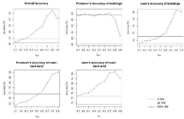
It is necessary to analyse the influence of the weight SMP on the classification
accuracy. A sensitivity analysis was performed in experiment I, in which the overall accuracy, together with the user’s and producer’s accuracies of the classes of buildings and road/bare land, was calculated while varying the weight SMP from 0.1 to
0.9 (Figure 8). As revealed in the error matrix, although the MPk-NN method does not yield the greatest accuracy consistently for each class, the overall accuracy is larger than for the other methods when SMP varies from 0.3 to 0.9. The accuracy decreases
when SMP reaches a certain value. Therefore, SMP was taken as 0.8 because it resulted
in the greatest overall accuracy.
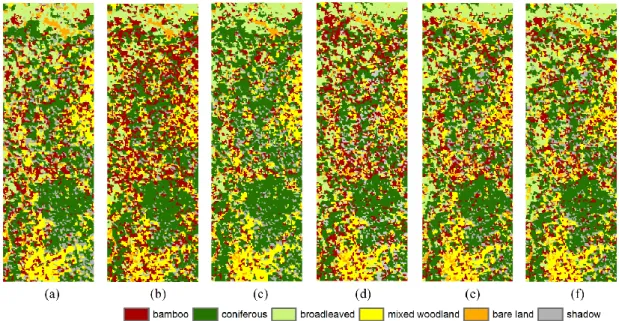
In the second experiment, the complex environment makes mapping of the distribution of the bamboo class challenging. As can be seen, the overall accuracy of the MPk-NN method is the greatest, whereas the Bayesian method produced the lowest overall accuracy. Bamboos appear more in the DTC result since the bamboo class has the most training samples and this may affect the classification. Although the DTC method resulted in a greater producer’s accuracy than the other methods due
11
to more bamboos being classified, it produced the lowest user’s accuracy. The Bayesian and SVM methods allocate fewer objects to the bamboo class than the others. The producer’s accuracies of the bamboo class are rather low, but the user’s accuracy is 61.29% using the SVM method, which is greater than for most methods. It indicates that most locations identified as bamboo using the SVM method are correct, but high omission errors occur, most probably missed in the coniferous area.
The k-NN method, interestingly, does not produce a greater accuracy than the other non-contextual classification methods (in contrast to the first experiment). The gk-NN and MPk-NN methods increased the accuracy of the bamboo class compared to the
k-NN method due to the introduced spatial weightings. For the MPk-NN method, the user’s accuracy of bamboo is above 65%, which is greater than for the other methods. However, the producer’s accuracies for coniferous woodland are lower using the three
k-NN methods than for the Bayesian, DTC, and SVM methods. More bamboos are mixed with the large patch of coniferous woodland in the lower right part of the image in the three k-NN results and this may be one reason for the lower coniferous woodland accuracy. The average accuracies of the broadleaved class are all above 80%, and the three k-NN methods produced a greater accuracy for mixed woodland than the other methods. MPk-NN produced the greatest accuracies for bare land and shadows. The spatial distributions of the bamboo, bare land and shadows classes are sparse and isolated, whereas the coniferous, broadleaved and mixed woodland classes have more connected distributions. Generally, the MPk-NN method increased the accuracy of the k-NN classifier targeted to those sparsely distributed classes. This is because the spatial weighting derived using MPS can work effectively for small areas, and strengthen the available spatial information by counting replicates of the observed spatial patterns.
4 Discussion
4.1 Choosing appropriate datasets
The technique proposed here is a general LCLU classification scheme based on the OBIA approach, and it is applicable to the same scenarios to which one would apply the standard OBIA approach. The prime requirement for the OBIA approach is that the LCLU objects of interest are resolvable given the spatial resolution of the imagery. Specifically, the relationship between the object sizes and the spatial resolution dictates whether the technique is appropriate for a given LCLU classification task. The actual spatial resolution of the imagery is important only in relation to the objects of interest, and in this sense, the technique is applicable to a broad range of LCLU applications and types of imagery with different spatial resolutions.
In the two examples in this paper the technique was demonstrated on images with a very fine spatial resolution. In one case, the objective was to classify an urban area in Beijing in which the classification of building objects was a component of the task,
12
and in the other case the objective was to classify a vegetated area in Sichuan Province, China in which the classification of areas of bamboo (as spatial objects) was a component of the task. In both cases, the spatial resolution was chosen to be sufficiently fine to resolve the (multiple) objects of interest.
The benefits of undertaking two different experiments are that the new approach is tested in two very different contexts, with different land cover types and using images with different spatial resolutions. However, the technique would be equally applicable to classification where the objects of interest were much larger and, thus, the appropriate spatial resolution was much coarser. For example, the classification of tropical rainforest across the whole of the Amazon Basin, including the identification of deforested areas, would require a coarser spatial resolution depending on the specific requirements, for example, the 250 m spatial resolution of the Moderate Resolution Imaging Spectrometer (MODIS). Thus, although the two specific examples required fine spatial resolution imagery, this need not be the case in alternative applications. In this sense, the MPS-based OBIA approach proposed here is as general as the popular OBIA approach and should be of utility in a wide variety of applications that require LCLU mapping.
4.2 Training image analysis
An open question in MPS is how best to select the training image. Here, a pre-classified map produced using the wk-NN method was selected as the training image. Using a pre-classified map as a training image is not a common choice in MPS. However, it should be noted that the MPk-NN method does not use this pre-classified map as a starting point for further updating. It only borrows spatial structure information, at varying spatial resolutions, from the pre-classified map to update the gk-NN classified map. Therefore, extraction of spatial structures from the training image is similar to a post-processing operation. In this sense, which classifier is used to produce the map for training is of little concern. In fact, training images produced manually or from different sources have been used in many studies related to MPS. Here, we used a previously classified image as the training image to avoid introducing new data. This has the advantages of providing a fair comparison with the benchmark methods and, at the same time, increasing the interpretability of the results.
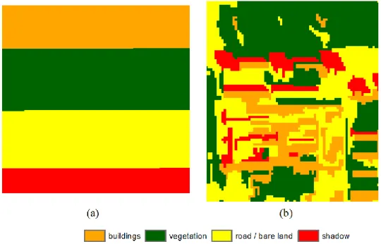
A test was performed to show the effects of the training image on the MPk-NN result. Only experiment I was tested since it involved more reference data. In the worst situation, a training image with the simplest spatial pattern was used, which honours only the proportions of the four classes, but does not reflect the spatial distribution (Figure 9a). Another training image used is a subscene of the IKONOS image. It was classified and revised manually to represent a similar class distribution to that of the study area (Figure 9b). The accuracy of the corresponding MPk-NN result using the first training image is 80.07%, equalling the accuracy of the gk-NN method, which means that no additional useful information was provided by this training image. The second training image led to an accuracy of 86.58% for the MPk-NN result. Here, the increased accuracy arises from the spatial structure of the training image representing
13
a new area, rather than from a pre-classified image of the same area.
4.3 Multiple-point probability
The data event determined by the shape of the template and the k-NN classes represents a certain type of spatial distribution. The frequency of the data event is then converted to spatial information that affects the k-NN classifier combined with spectral information. The spatial information of MPS is, thus, different from the spatial covariance provided by traditional geostatistics in three ways. Firstly, the multiple-point probability is not estimated as a function of distance. Thus, data values may have a large effect via the spatial weighting, even if the k-NN nodes are far from the central segment in geographical space. Secondly, the spatial covariance measures the spatial correlation between the central segment and one of its k-NN nodes at one time; MPS summarises the correlation of the central segment and all of its k-NN nodes. Finally, the weight factor SMP accounts for more weight than Sg; so if SMP is too
large it may reduce the accuracy.
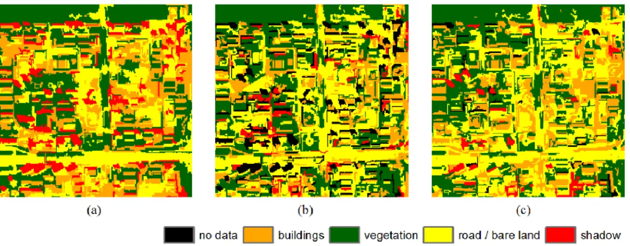
It is of interest to explore the patterns captured using the data template. Figure 10 shows the categorical maps in experiment I, in which the classes correspond to the maximum multiple-point probabilities, with multi-grid level L equal to 1, 2 and 3. Since the image used for training is of the same area, one potential problem is that scanning the training image leads to a high frequency of matches within the spatial extent of the object where the data template is defined. In this case, replicates of the data event can be found only using the original data template (Figure 10a). Thus, the multi-grid template was used to check if spatial information can be captured when changing the shape (size) of the data template. It can be seen that although replicates of data events were not found in some places, the pattern generally shows a similar distribution to that of the classification maps. Most places without matched data events are shadows in Figure 10b and c. This is because shadows are isolated and account for only a small proportion of the total area and, thus, can easily be missed by a smaller template. This problem is avoided when applying MPk-NN at the pixel level. Another alternative to this problem is to reduce the K value for the data template to relax the matching conditioning.
5 Conclusion
The research presented here explored the potential of MPS for spatially weighting a remote sensing classifier generally and, in the present case for the first time, for the highly popular OBIA classification. A multiple-point statistical k-NN classification method was tested on remote sensing images of an urban area and a mountainous area. The MPk-NN classifier borrows spatial structure from multiple parts of a training image to condition the classification of an input image. The proposed method can account for spatial correlation at multiple points simultaneously, in contrast to common spatial weighting schemes, which are limited to two-point statistics. The
14
experiments demonstrated the advantage of the MPS approach compared to a geostatistical weighting. Specifically, the results demonstrate that greater classification accuracy can be achieved using the proposed new weighting scheme compared to five alternative methods. Future research should be directed towards: (i) analysis of the choice and nature of training image; (ii) the method of conversion from objects to points to support location- and distance-based spatial weighting and (iii) development of a self-adaptive method for parameter estimation.
Acknowledgements
The publication of this paper was supported by the 100 Talents Program of the Chinese Academy of Science [grant number Y34005101A], the National Natural Science Foundation of China [grant number 41501489], the National Science and Technology Support Program [grant number 2013DFG21640], and the Major Program of High Resolution Earth Observation System [grant number 30-Y20A37-9003-15/17]. The authors thank two anonymous reviewers for providing helpful suggestions that greatly improved the manuscript.
15
References
Armstrong, M., 1998. Basic Linear Geostatistics. Berlin, Germany: Springer-Verlag, pp. 35.
Atkinson P.M., Lewis, P., 2000. Geostatistical classification for remote sensing: an introduction. Comput. Geosci. 26(4), 361-371.
Atkinson, P.M., Naser, D.K., 2010. A geostatistically weighted k-NN classifier for remotely sensed imagery. Geogr. Anal. 42(2), 204-225.
Blaschke, T., Strobl, J., 2001. What’s wrong with pixels? Some recent developments interfacing remote sensing and GIS. GIS – Z. Geoinf. Sys.14(6), 12-17.
Boucher, A., 2009. Sub-pixel mapping of coarse satellite remote sensing images with stochastic simulations from training images. Math. Geosci. 41(3), 265-290. Dudani, S.A., 1976. The distance weighted k-nearest neighbour rule. IEEE Trans. Syst.
Man Cybernet. SMC-6(4), 325-327.
Ge Y., Bai, H., 2011. Multiple-point simulation-based method for extraction of objects with spatial structure from remotely sensed imagery. Int. J. Remote Sens. 32(8), 2311-2335.
Jensen, J.R., 1979. Spectral and textural features to classify elusive land cover at the urban fringe. Prof. Geogr. 31(4), 400-409.
Johnson, B., Xie, Z., 2013. Classifying a high resolution image of an urban area using super-object information. ISPRS J. Photogramm. Remote Sens. 83, 40-49.
Myint, S.W., Gober, P., Brazel, A., Grossman-Clarke, S., Weng, Q., 2011. Per-pixel vs. object-based classification of urban land cover extraction using high spatial resolution imagery. Remote Sens. Environ. 115(5), 1145-1161.
Newman, M.E., Mclaren, K.P., Wilson, B.S., 2011. Comparing the effects of classification techniques on landscape-level assessments: pixel-based versus object-based classification. Int. J. Remote Sens. 32(14), 4055-4073.
Okabe H., Blunt, M.J., 2005. Pore space reconstruction using multiple-point statistics. J. Petrol. Sci. Eng.46(1-2), 121-137.
Park, N.W., Chi, K.H., Kwon, B.D., 2003. Geostatistical integration of spectral and spatial information for land-cover mapping using remote sensing data. Geosci. J. 7(4), 335-341.
Pasolli, E., Melgani, F., Tuia, D., Pacifici, F., Emery, W.J., 2014. SVM active learning approach for image classification using spatial information. IEEE Trans. Geosci. Remote Sens. 52(4), 2217-2233.
16
geostatistical simulation for post-processing a remotely sensed land cover classification.Spat. Stat.5, 69-84.
Tran, T., 1994. Improving variogram reproduction on dense simulation grids.Comput. Geosci. 20(7-8), 1161-1168.
Wang, G., Liu, J., He, G., 2013. A method of spatial mapping and reclassification for high-spatial-resolution remote sensing image classification. The ScientificWorld Journal, 192982.
17
Figures and Tables
Figure 1. A cross-shaped data template extracts data events from a training image. (a) Template and data event (b) Training image (c) Matched data event
18
19
Image segmentation Remote sensing
imagery
Data template with multi-grid level L Initial classification Training samples Find K nearest segments in feature space Identify centroid locations of K segments in geographical space Training image
Find data event matches and record
the central class Estimate multiple-point probabilities by counting the replicates Incorporate into the
gk-NN classifier Scan the training
image by data template MPk-NN classification result Yes L = 1? L = L– 1 No
20
Figure 4. Image of study area and sample points in Beijing: (a) IKONOS image (true colour composite) and reference data, (b) training segments selected for classification, (c) training points for geostatistical modelling (unit: pixel).
21
Figure 5. Image of study area and sample points in Wolong: (a) WorldView-2 image of Dengsheng Ditch (true colour composite), (b) training sample segments, and (c) reference data.
22
Figure 6. Classification in Beijing using six methods: (a) Bayesian, (b) DTC, (c) SVM, (d) k-NN, (e) gk-NN, and (f) MPk-NN.
23
Figure 7. Classification in Wolong using six methods: (a) Bayesian, (b) DTC, (c) SVM, (d) k-NN, (e) gk-NN, and (f) MPk-NN.
24
Figure 8. Plots of accuracies against SMP weighting between 0.1 and 0.9 for the
25
Figure 9. Different training images: (a)the simplest pattern, and (b) a classified subset of the IKONOS image.
26
Figure 10. Categorical maps corresponding to the maximum multiple-point probability in Beijing, with different multi-grid levels: (a) L = 1, (b) L = 2 and (c) L = 3.
27
Table 1. Classification accuracies of the Bayesian, DTC, SVM, k-NN, gk-NN and MPk-NN methods in Beijing. Class name: 1-buildings, 2-vegetation, 3-road/bare land, 4-shadow.
Method Class User’s
accuracy (%) Producer’s accuracy (%) Overall accuracy (%) Kappa coefficient Bayes 1 51.85 53.85 70.65 0.599 2 95.65 100 3 58.95 65.88 4 100 65.96 DTC 1 70.51 70.51 75.72 0.671 2 96.08 74.24 3 66.67 72.94 4 79.63 91.49 SVM 1 31.82 8.97 67.03 0.550 2 96.97 96.97 3 48.25 81.18 4 100 95.74 k-NN 1 65.59 78.21 80.07 0.731 2 98.44 95.45 3 71.23 61.18 4 97.83 95.74 gk-NN 1 62.39 87.18 80.07 0.731 2 98.46 96.97 3 77.19 51.76 4 100 95.74 MPk-NN 1 93.42 91.03 94.93 0.931 2 94.29 100 3 93.98 91.76 4 100 100
28
Table 2. Classification accuracies of the Bayesian, DTC, SVM, k-NN, gk-NN and MPk-NN methods in Wolong (Class name: 1-bamboo, 2-coniferous, 3-broadleaved, 4-mixed woodland, 5-bare land, 6-shadow).
Method Class User’s
accuracy (%) Producer’s accuracy (%) Overall accuracy (%) Kappa coefficient Bayes 1 46.67 33.33 75.34 0.699 2 75.86 81.48 3 85.00 94.44 4 76.09 77.78 5 81.82 94.74 6 85.19 85.19 DTC 1 52.17 57.14 76.23 0.709 2 76.67 85.19 3 80.95 94.44 4 79.41 60.00 5 90.00 94.74 6 100 77.78 SVM 1 61.29 46.34 78.90 0.743 2 73.21 82.00 3 81.40 97.22 4 87.18 75.56 5 88.89 84.21 6 87.10 100 k-NN 1 53.49 54.76 77.58 0.727 2 74.51 70.37 3 81.40 97.22 4 94.29 73.33 5 94.44 89.47 6 81.82 100 gk-NN 1 56.10 54.76 78.92 0.743 2 76.47 72.22 3 83.33 97.22 4 87.50 77.78 5 89.47 89.47 6 90.00 100 MPk-NN 1 65.71 54.76 80.72 0.764 2 80.00 81.48 3 77.78 97.22 4 85.37 77.78 5 94.12 84.21 6 90.00 100
29
Table 3. ANOVA for the classification methods in Beijing with respect to the MPk-NN method using F-test.
Method F-ratio Significant at 90% level
F-value 2.71 Bayes 63.43 Yes DTC 43.71 Yes SVM 79.52 Yes k-NN 29.22 Yes gk-NN 29.22 Yes