Network Traffic Based Botnet Detection Using Machine Learning

SJSU ScholarWorks

SJSU ScholarWorks

Master's Projects Master's Theses and Graduate Research

Spring 5-18-2020

Network Traffic Based Botnet Detection Using Machine Learning

Network Traffic Based Botnet Detection Using Machine Learning

Follow this and additional works at: https://scholarworks.sjsu.edu/etd_projects

Part of the Artificial Intelligence and Robotics Commons, Information Security Commons, and the OS and Networks Commons

Network Traffic Based Botnet Detection Using Machine Learning

A Thesis

Presented to

The Faculty of the Department of Computer Science San Jose State University

In Partial Fulfillment

Of the Requirements for the Degree Master of Science

By

Anand Ravindra Vishwakarma May 2020

The Designated Project Committee Approves the Project Titled

Network Traffic Based Botnet Detection Using Machine Learning

by

Anand Ravindra Vishwakarma

APPROVED FOR THE DEPARTMENT OF COMPUTER SCIENCE

SAN JOSE STATE UNIVERSITY

May 2020

Dr. Robert Chun Department of Computer Science Dr. Chris Pollett Department of Computer Science Mr. Abhishek Sharma Twitter, Inc

i

ABSTRACT

The field of information and computer security is rapidly developing in today’s world as the number of security risks is continuously being explored every day. The moment a new software or a product is launched in the market, a new exploit or vulnerability is exposed and exploited by the attackers or malicious users for different motives. Many attacks are distributed in nature and carried out by botnets that cause widespread disruption of network activity by carrying out DDoS (Distributed Denial of Service) attacks, email spamming, click fraud, information and identity theft, virtual deceit and distributed resource usage for cryptocurrency mining. Botnet detection is still an active area of research as no single technique is available that can detect the entire ecosystem of a botnet like Neris, Rbot, and Virut. They tend to have different configurations and heavily armored by malware writers to evade detection systems by employing sophisticated evasion techniques. This report provides a detailed overview of a botnet and its characteristics and the existing work that is done in the domain of botnet detection. The study aims to evaluate the preprocessing techniques like variance thresholding and one-hot encoding to clean the botnet dataset and feature selection technique like filter, wrapper and embedded method to boost the machine learning model performance. This study addresses the dataset imbalance issues through techniques like undersampling, oversampling, ensemble learning and gradient boosting by using random forest, decision tree, AdaBoost and XGBoost. Lastly, the optimal model is then trained and tested on the dataset of different attacks to study its performance.

Index Terms: Botnet Detection, Feature Selection, Imbalanced Learning, Machine Learning, XGBoost.

ii

ACKNOWLEDGMENTS

I would like to thank my advisor, Dr. Robert Chun, for his continued guidance and support in successfully completing this project through his experience and research knowledge.

I would also like to extend my gratitude towards my committee members, Dr. Chris Pollett and Mr. Abhishek Sharma for giving their time and support.

Lastly, I would like to thank my parents, relatives, and friends for always supporting and believing in me.

iii

TABLE OF CONTENTS

I. Introduction ... 1

II. Understanding Botnet ... 5

A. Configuration ... 5

B. Architecture ... 5

III. Botnet Attacks And Types ... 7

A. Lifecycle ... 7

B. Attack Methods ... 7

1.) Denial of Service (DoS) or Distributed Denial of Service (DDoS): ... 7

2.) Miscellaneous Attacks: ... 8

IV. Botnet Detection Methods ... 9

A. Classical Methods ... 9

B. Signature and Anomaly Based ... 9

C. Machine Learning-Based ... 11 D. Deep Learning-Based ... 14 V. Dataset ... 17 A. CTU-13 Dataset ... 17 B. Dataset Features ... 18 C. Descriptive Analytics ... 19 VI. Preprocessing ... 21

A. One Hot Encoding ... 21

B. Label Encoding ... 21

C. Dropping Columns ... 22

D. Scaling... 22

VII. Feature Selection ... 23

A. Removing Null Columns ... 23

B. Variance Thresholding ... 24

C. Filter Methods ... 24

D. Wrapper Methods ... 26

E. Embedded Methods ... 27

F. Feature importance and Correlation Heatmap ... 28

VIII. Addressing Data Imbalance ... 30

iv

B. Oversampling ... 31

C. Oversampling followed by Undersampling ... 32

D. Ensemble Learning ... 33

E. Cost-Sensitive Learning - XGBoost ... 34

IX. Machine Learning Classifiers ... 35

A. Decision Tree ... 35

B. Random Forest ... 35

C. AdaBoost... 36

X. Technology Stack ... 37

A. Hardware ... 37

B. Software and Libraries ... 37

XI. Implementation ... 38

XII. Evaluation Metrics ... 39

A. Classification Report ... 39

B. ROC Curve ... 40

XIII. Experiments ... 41

A. Baseline Model ... 41

B. Feature Reduced Model ... 42

1.) Strategy 1: All Features ... 43

2.) Strategy 2: Variance Thresholding... 44

3.) Strategy 3: Reduced Classes ... 44

C. Oversampled Models ... 46

D. Undersampled Models ... 47

E. Oversampled + Undersampled Models ... 48

F. Ensemble Learners ... 49

G. Cost-Sensitive Model – XGBoost ... 50

H. XGBoost on all 13 scenarios ... 52

XIV. Results ... 53

XV. Conclusion ... 54

v

LIST OF FIGURES

Figure 1: Conceptual Map of Project ... 4

Figure 2: Traffic Frequency Distribution ... 20

Figure 3: Protocol Frequency Distribution ... 20

Figure 4: Variance Thresholding ... 24

Figure 5: Flow Diagram for Filter Methods ... 25

Figure 6: Flow Diagram for Wrapper Methods ... 27

Figure 7: Flow Diagram for Embedded Methods ... 28

Figure 8: Correlation Heatmap Matrix ... 29

Figure 9: Illustration of Undersampling [22] ... 31

Figure 10: Illustration of Undersampling - Tomek Links [23] ... 31

Figure 11: Illustration of Oversampling [22] ... 32

Figure 12: Illustration of SMOTE [26] ... 32

Figure 13: XGBoost Model ... 34

Figure 14: Illustration of Decision Tree ... 35

Figure 15: Illustration of Random Forest ... 36

Figure 16: Illustration of AdaBoost ... 36

Figure 17: Illustration of Confusion Matrix ... 40

Figure 18: Interpretation of the ROC Curve ... 40

Figure 19: Frequency Distribution of Categorical Columns ... 41

Figure 20: Confusion Matrix for RFC and DT ... 46

Figure 21: Ensemble Learners Performance Comparison ... 50

Figure 22: XGBoost ROC-AUC Score ... 51

vi

LIST OF TABLES

Table 1: Dataset Scenario Description ... 17

Table 2: Dataset Diversity Distribution ... 18

Table 3: Feature Columns Description ... 19

Table 4: Continuous Features Statistics ... 22

Table 5: Baseline Model ROC-AUC Scores ... 42

Table 6: Feature Selection on Strategy1 Dataset ... 43

Table 7: Feature Selection on Strategy2 Dataset ... 44

Table 8: Feature Selection on Strategy3 Dataset ... 45

Table 9: Oversampling Results ... 47

Table 10: Undersampling Results ... 48

Table 11: Ensemble Learners Performance ... 49

Table 12: ROC Curve for XGBoost on 5 and 10 Features of Strategy1 Dataset ... 50

1

I. INTRODUCTION

The internet is plagued with information theft and security risks. Information theft includes personal details stolen to conduct identity fraud, and debit and credit card credentials traded on the dark web to carry out illicit transactions. Some of the security risks include but are not limited to systems, servers, and networks compromised with malware, trojan horses, phishing, ad-wares, deceive, ransomware, and viruses [1]. While accessing resources like audio, video, and images and surfing the internet, users are targeted with unwanted ads, spam notification, and emails and denial of service. The attacks mentioned are carried out in a distributed manner for illegal purposes, monetary gains, to create biasedness among public opinion and harm the organization’s reputation [1, 2].

Botnet comprises 80% of the attacks on the internet in the modern world. These nefarious activities are well organized and carried out by a hacker. A botnet is a network of malware compromised computers (called as bot or zombie) under the control of a hacker (also called as botherder or bot-master). A botherder controls the bots by using a Command and Control server (C&C). Identifying the vulnerable systems, propagating the malware, sending the command, and code updates and carrying out the attack are primarily controlled by the C&C server. A collective effort from the botnet attacks can result in Distributed Denial of Service (DDoS), phishing, spamming, spreading of malware, information theft, unwanted ads, generating virtual clicks and cryptocurrency mining. Prevention or detection of botnet attack is difficult because of its inherent nature of changing the attacks modus operandi [2].

Many types of research have been done to effectively and successfully detect and block botnet attacks. The goal of this project is to propose a machine learning model to detect botnets with

2

better precision and reduce false positives by studying existing work done in the botnet detection area. The articles selected for this project include conference proceedings, articles and, published papers. This project tries to answer the following questions:

1. To what length the existing botnet detection methods are successful and their fallacies over each other?

2. What selection method can help us in identifying the optimal set of features for efficient and accurate model training?

3. How the dataset imbalance issue of botnet originated traffic can be handled?

4. Is there any machine learning model that can detect a range of botnet attacks?

The literature establishes that there does not exist a single strategy that can work across all types of botnet attack as identified in previous works. Selection methods work well on datasets with fewer columns obtained after variance thresholding and one hot encoding. The handling of botnet dataset imbalance is well done by using an undersampling strategy and bagging classifiers with implicit imbalance handling. XGBoost emerges as a model in this project that scales well to a wide range of botnet attacks.

The remaining section of the review is organized as follows: Section II focuses on architecture, the configuration of botnets. Section III delineates the attack phase and widely known attack methods. Section IV examines the classical methods of botnet detection and its failure and contrasts it with various bettered methods of signature and anomaly-based detection. It also reviews the contribution of machine learning and deep learning techniques in successful botnet detection. Section V introduces the dataset under consideration and provides an overview of the dataset using descriptive analytics. Preprocessing steps for dataset cleaning are mentioned in section VI. Section VII focusses on the feature selection techniques for reducing the feature space

3

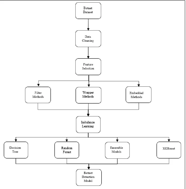
to improve model training time. The imbalance issue in the botnet dataset ecosystem and the approaches that can be adopted to balance the dataset is mentioned in section VIII. Section IX and X identify the machine learning classifiers that have been used and the technology stack in terms of software and hardware. A brief description of implementation can be found in Section XI. The evaluation metrics to measure the performance of the model is specified in section XII. A wide range of experiments conducted on the botnet dataset using feature selection and imbalance learning on machine learning classifier is explained in section XIII. The entire summary of the experiments in the form of results can be found in Section XIV. Section XV introduces the conclusion and section XVI ends with the future scope of the project. The entire project will follow the conceptual map as shown in Figure. 1.

4

5

II. UNDERSTANDING BOTNET

As previously discussed in the introduction, Botnet is a network of infected computers responsible for carrying out distributed attacks [2]. In this section, we delve into exploring the architectures and configuration of the botnet and its lifecycle.

A. Configuration

Various configurations or topologies that can be summarized into below four categories are described in [2-7] and [8]. In this star or Centralized C&C Topology, there is a single server (botmaster) that communicates with all the botnet members. Failure of the server can cause disruption of the botnet. Legacy botnets are based on this type of architecture but, recently shift has been made towards P2P architectures. To make botnet fault-tolerant, instead of a standalone server, multiple servers work in tandem to coordinate attacks, malware distribution, and weak system identification by sending commands to bots in Multi-Server C&C Topology. Hierarchical C&C Topology as the name implies has a central botmaster that controls bot and then the bot assumes the role of botmaster and in turn controls its botnet members and so on. In Peer-to-Peer topology there is no central server, instead, every bot member is capable enough to do tasks of a botnet. In other words, every bot is a bot as well as a botmaster.

B. Architecture

Botnets are broadly classified based on the protocol used by command and control server into IRC-based, HTTP-based, DNS-based or Peer to Peer (P2P) botnets [2, 3, 4, 5, 6]. There are also some lesser-known botnet categories like POP-based botnets for email attacks, edge devices botnets like SMS and MMS-based botnet and social network botnets as specified in [7].

An IRC-based botnet used Internet Relay Chat Protocol (IRC) [3]. An IRC network is made up of multiple servers that work in co-ordination to relay messages across servers. Each server has

6

multiple channels that have published topics. A user connects to one of the IRC servers with a UNIQUE Id and then uses one of the channels to communicate. [3] explains that a channel in an IRC network is a bot (malware) and all the systems infected by the same malware belong to the same channel. On the other hand, an HTTP-based botnet (also known as Web-based botnet) relies on HyperText Transfer Protocol (HTTP) for its communication with the bot members. [4] specifies that most of the internet traffic is HTTP traffic and HTTP-based botnets clearly take advantage of this and disguise themselves as normal traffic. Compared to IRC-based botnet [3], [4] explains HTTP-based botnet are relatively difficult to detect primarily for two reasons: first they hide behind normal traffic and second, most of the firewall/proxies do not have the capability for deep packet inspection (examine network packet at each layer).

A DNS-based botnet utilizes the Domain Name System protocol (DNS) useful for contacting the C&C server by issuing DNS queries. DNS systems are a directory of IP addresses responsible for converting Domain Name into IP addresses (also called as domain name resolution) and vice-versa. [5] delineates that the bots and botmaster communicate by using DNS queries and in order to avoid detection, the C&C server keeps changing the domain name by using Domain Generation Algorithm (DGA) or fast-flux which makes them robust to detection. Newly generated IP and domain names are constantly being updated in the DNS system. In comparison to IRC-based, HTTP-based, and DNS-based, which uses client-server architecture as specified in [3, 4, 5], P2P-based botnet uses peer to peer network in a distributed fashion which makes them robust for detection. Since, there is no single master, every bot in the network is a master and capable of infecting vulnerable systems and carry out the attack. [6] examines various P2P traffic types and concludes that P2P-based detection is difficult owing to its inherent distributed nature.

7

III. BOTNET ATTACKS AND TYPES

A. Lifecycle

Botnet lifecycle comprises of five stages as specified in [1, 2, 7]. In the initial Infection stage, the C&C server scans the network and looks for vulnerabilities in the network, servers, and system. Obvious flaws like buffer overflow, backdoors, incomplete mediation, password guessing on SQL servers are done. Once the weak systems are identified, they are targeted with a shell script and run on it in the secondary infection stage. The shell scripts enable the systems to download malware or bot binary codes from the C&C server. In the connection stage, once the malware is run on the host system, a connection is established to the C&C server and the botmaster can now send the commands to the system and is now a part of the botnet. In Malicious Command and Control phase, the C&C server sends attack commands to the botnet members to disrupt online services. The update and maintenance phase is an ongoing process that is required as a C&C server in order to avoid detection it keeps migrating the server.

B. Attack Methods

Botnet attacks are motivated by various reasons like economic, political and ideological considerations. Sometimes, extortion or ransom, personal feuds, naïve enthusiasts or script kiddies and cyber warfare could be the possible reasons for such attacks.

1.) Denial of Service (DoS) or Distributed Denial of Service (DDoS):

Denial of service is a kind of attack in which the target resource is inundated with many requests which overwhelm the target making it unavailable to the user. Generally, DoS is executed by a single machine and it is not capable enough to bring down the target system. Practically, multiple machines are required to launch such attacks, hence DDoS attacks are ubiquitous and difficult to break down [1, 2]. [8] broadly classifies DDoS attacks into three

8

categories: volume-based attacks, protocol attacks, and application-layer attacks. Volume-based attacks include UDP flood and ICMP flood. A UDP flood is any DDoS attack that uses User Datagram Protocol (UDP) packets to bring down the network by rapidly sending spoofed UDP packets to the host. The host in response sends error messages since spoofed packets do not have any legit connections. ICMP (Internet Control Message Protocol) flood is also known as a ping attack in which diagnostic tools like traceroute or ping are used to check the device health and connectivity. Many ping requests will require the same number of responses and make the device crash.

2.) Miscellaneous Attacks:

The Spamming and Traffic Monitoring attack include bots that are used as a sniffer to steal sensitive data like usernames and passwords from the infected machines. Internet users are targeted with spam emails that are sent out in bulk using botnets such as Grum responsible for 25% of the total spam emails. With the help of botnet, bots can spread out keyloggers which are software that captures key sequence presses on the keyboard and designed in such a way that gets activated when popular keywords like PayPal and Yahoo are entered. Spam emails are disguised as legit emails that direct users to legitimate websites to enter bank details, tax details, personal details, and card details. Such information is traded on the dark web for fees. Pay-per-click is one of Google’s AdSense program in which various websites display Google advertisements and earn money when the user clicks on those ads. Botnet, apart from carrying out attacks, also has the potential to propagate botnet over various geographical regions by targeting less secure systems. Adware is harmless ads but in disguise collects browser data by using spyware software. It is used to lure users into clicking false advertisements or apps with the pretext of monetary or personal profits.

9

IV. BOTNET DETECTION METHODS

In this section, we will dive deep into the traditional botnet detection method, state of the art detection method followed by an amalgamation of machine learning, and deep learning techniques for detecting botnet.

A. Classical Methods

A honeypot is a computer system that is placed in the DMZ (Demilitarized Zone) network of the company that is used to lure the attackers into attacking it [8]. A honeypot is a vulnerable system and any communication between honeypot and outside the system is considered suspicious. [1, 2] broadly studied the concept of honeypot and identified that the system used as honeypot does not have any production value. A typical honeypot captures information such as the signature of the bot (malware), C&C server mechanism, botnet details, techniques used by the attacker, attacker motivation and most importantly, the loophole of the system that bot exploited. Apart from discussing the simplicity of the model, [1, 2, 7] also enlightened on the limitations associated with the honeypots. Honeypots (or Honeynet) have limitations in detecting several exploitations, bots that use propagation, cannot scale to other malicious attacks, and it can only generate a report of the attack on the honeypot system. It cannot detect the attack in real-time as well as bot attacks on some other system.

B. Signature and Anomaly Based

Intrusion Detection System (IDS) is the emerging field in botnet detection as an alternative to Honeypots. IDS systems are classified as signature-based and anomaly-based detection. Recent works in botnet detection as described in [10 – 15], utilizes the different mechanisms of anomaly-based detection as compared to signature-anomaly-based detection. Signature-anomaly-based IDS maintains a database of attack signature and uses it to scan and compare the incoming traffic against the

10

available signatures. Immediate detection and zero false-positive rates as noted in [9] are the benefits of signature-based IDS. They are useful in the sense the exact cause of the attack is also known in IDS Response and the network administrators can take appropriate steps by quarantining the segment of the network or the infected system. [8] notes some of the associated disadvantages like detection time decreases as the signature database increases in size, the signature needs to be updated on daily basis, cannot detect variant of the botnet attack and cannot identify zero-day attacks or new botnet. [10] renders signature-based IDS as ineffective owing to modern botnets being equipped with advanced code patching and dodging techniques. Due to its inherent nature of being static, anomaly-based detection techniques are widely implemented.

Research has shown that anomaly-based techniques are much better at detection as it does not require a database of signature and is capable enough to detect new or unknown botnets. Anomaly-based techniques try to detect botnet by using various network characteristics like network protocols, packet size, stateful and stateless features, traffic size, unusual system, and abnormal behaviors. They are implemented as either host-based IDS or network-based IDS as explained in [9]. A host-based IDS is implemented on the system and is unaware of the network traffic whereas a network-based IDS is unaware of host network traffic. Anomaly-based detections detect behavior that goes out of normal behavior. Due to this feature, Anomaly-based IDS is effective in identifying new or variant of existing botnets in real-time. Surveys on Anomaly-based IDS in [1, 2, 7, 8, 9] has confirmed that anomaly-based IDS cannot be used as a foolproof measure of detecting botnet because as it is difficult to identify the normal threshold and also the network activity changes over time and hence, the IDS has to evolve. Also, such systems cannot effectively reveal the specific type of attack which makes it difficult to block the botnet. Hence, hybrid systems of Anomaly and Signature-based implementation are widely used in insecure networks.

11 C. Machine Learning-Based

The field of machine learning and deep learning is now the most widely implemented and experimented area. [10 – 15] have described various techniques of botnet detection using machine learning or deep learning in combination with botnet characteristics.

Botnet detection using machine learning techniques like k-NN (k-Nearest Neighbor), Decision Tree (DT), Random Forest (RF), and Naïve Bayes model based on DNS Query data is mentioned in [10]. Bots of the botnet receive code and commands from the C&C server by performing lookup queries generated using DGA or fast-flux. [10] identifies that the IP address of the C&C server is not a legit name and keeps on randomly changing to avoid detection. Also, the generated malicious domain names have characteristics like DNS, network and lexical features entirely different from benign domain names. [10] approaches to solve the problem by collecting 16 vocabulary features from 2-g and 3-g clusters like mean, variance, standard deviation, entropy, consonants, vowels, number, and character characteristics and 2 characteristics from vowel distribution. IP addresses are random with datasets generated from Conficker, and DGA botnet (malicious) and top domain names from Alexa Internet (benign) (collection of domain names) in conjunction with machine learning models, [10] demonstrated the effectiveness of Random Forest machine learning model by delivering an accuracy of 90.80% in botnet detection. Also, the proposed random forest-based detection system suffered from a relatively high false-positive rate. Some related research papers to [10], [16] implemented techniques for detecting botnets by administering the DNSBL (Domain Name System Blacklist) list which contains IP addresses of spam bot members and matching it with DNS queries domain names. [17] extends its work on the idea that most of the DNS queries are made to terminated domains or NXDOMAIN (non-existent domains) as the C&C server keeps

12

on changing the IP addresses and it was successful in detecting traffic with a large number of queries and terminated domains.

Botnet detection models in the works of literature are heavily built for network and network devices as discussed in [10, 16, 17]. Work expressed in [14] proposes a detection model for the Internet of Thing (IoT) devices by highlighting the fact that IoT specific behaviors are unique like they have few endpoints for connections and the time interval between the packet is well regulated. It postulates that botnets such as Mirai are exploiting insecure IoT devices to carry out DDoS attacks in large numbers. A recent survey in [1, 2] predicts that by 2020, the number of IoT devices will be around 20 billion and 10% of these devices have flaws ranging from un-encrypted data transmission, outdated BIOS firmware, and exposed telnet ports. [14] considers Random Forest, k-nearest neighbors, Decision Trees, SVM and neural network and train these models on network flow parameters like length of the packet, size of the interval and protocol used. The detection pipeline is flow-based (considers network behavior), uses either stateless or stateful features and is protocol-agnostic (robust to different protocols). [14] expresses the issues surrounding IoT devices like lightweight characteristics, limited memory, and computation power. Steps involved in building an IoT-based detection model is capturing the traffic, grouping the packets based on device (stateful) and by time (study temporal patterns), extracting stateful and stateless features followed by a binary classification. [14] experimented with the dataset and found out that normal traffic packet size varies between 100 to 1200 bytes whereas attack traffic is under 100 bytes owing to repeated attacks. Also, the attack traffic has a lesser inter-packet interval in comparison to normal traffic. Most of the time protocols used during attack were TCP as opposed to UDP during normal situations. The classifiers were able to obtain training accuracy from 0.91 to 0.99. However, though the accuracy was 0.99, it was built on simulated data generated using DDoS

13

attack. [14] predicts the model might be overfitting the data but is unsure of its performance on real-time attacks which opens the door for future research in the detection of botnets.

Work was done in [11, 14] that focused on detecting botnet using IP address details and traffic flow characteristic, respectively. On the other hand [16] focusses on leveraging the detection of botnet using an efficient flow-based technique by reducing the packet size and time of traffic flow under consideration. The model was developed to detect two P2P botnets namely Storm and Waledac botnets during the honeynet project. It has been noted in many papers that modern botnets are resilient to detection by employing techniques like protocols obfuscation, encrypted communication, fast-flux and random domain name generation using DGA. P2P botnets have a disastrous effect on industrial systems and their infrastructures. In order to train the models, [16] captured network traffic of five tuples like source IP address, source port, destination IP address, destination port and protocol used. As well for every traffic, 39 other statistical features were extracted. [16] employed batch analysis and limited analysis of the captured traffic by using eight different machine learning algorithms like Naïve Bayesian Classifier (NB), Logistic Regression (LR), Bayesian Network Classifier (BNet), Linear Support Vector Machine (LSVM), Neural Networks, Random Forest Classifier, Random Tree Classifier, and Decision Tree Classifier. In the modeling process of botnet detection of [16], all MLA (machine learning algorithms) delivered impressive performance except Naïve Bayesian Classifier for both malicious as well as non-malicious traffic. The tree classifiers delivered promising classification performance, but Random Forest Classifier delivered the highest accuracy. Remaining MLAs experimented in [16], delivered the worst performance for non-malicious traffic as compared to normal traffic since the dataset was skewed in the former case. Additionally, [16] was successful in stating that high performance in detection was obtained by monitoring the traffic flow for only 60 seconds with an accuracy of

14

95%. Also, the initial 10 packets per flow are evident enough to detect botnet as opposed to monitoring the entire flow.

To summarize, [14] experimented with detecting botnet on consumer internet of thing device based attack. [11] considered a deep learning model, whereas [14] demonstrated the effectiveness of k-NN, Linear Support Vector Machine (LSVM), Decision Tree, Random Forest, and Neural Network by achieving an average accuracy of 99%. [14] also considered stateful features like bandwidth, and IP destination address cardinality and novelty and stateless features like packet size, inter-packet interval and protocols separately and together during the training phase. [15] employed flow-based machine learning technique for botnet detection and experimented with models like Naïve Bayes, Bayesian Net, Artificial Neural Network, Support Vector Machine, Random Tree, Random Forest, and Decision Tree. The flow-based model was able to achieve accurate detection of traffic only for 10 packets and 60 seconds of the flow. Next, we will consider the advancements done using Deep Learning for botnet detection.

D. Deep Learning-Based

Deep Learning is a research field and is constantly evolving. Recent researches in the detection of the botnet have shifted its gear towards building the model using Deep Learning techniques. Autoencoders, Long Short-Term Memory (LSTM) and Convolutional Neural Networks (CNN) have played a leading role in blocking attacks of a botnet. Next, we describe deep learning models developed for the detection of the botnet.

For botnet detection, [10] used a supervised learning model whereas [11] used an unsupervised learning model. Most of the detection models are built for botnet on the network, [11] focused on IoT devices that are more vulnerable to botnet attacks since they are relatively less secure owing to their size and computation requirements. This paper studies the effect of Mirai and BASHLITE

15

botnet attack on IoT devices by capturing network snapshots of traffic behavior emanating from malware attacked IoT devices. It promotes building a model that expedites the alerting process which can effectively help in quarantining the device as soon as possible and specifically for large scale enterprise networks where the number of connected IoT devices through Wi-Fi (Wireless Fidelity) and Bluetooth is extremely large. [11] develops a novel network-based model using deep learning-based autoencoder for each device which delivers a lower false-positive rate. The autoencoder is trained on benign network behavior (snapshots) and tries to compress it called an encoding phase. During the decoding phase, it tries to re-construct the snapshot, and failure to do so means an anomalous behavior is observed. [10, 14, 15] focus on initial stages of infection, [11] operated on the attack stage which provides benefits like heterogeneity tolerance (separate encoder for each device), efficiency (trains on a batch of observation and then discards it) and Open World (detect abnormal behavior). To build the model, [11] 23 features were obtained from 115 traffic statistics over the various time frame of varying minutes. Throughout the training process, hyperparameter learning was also performed followed by learning of threshold for abnormal behavior and effective window size. TPR for autoencoder was 100%, though it raised few false alarms and required the smallest detection time for most IoT devices. The deep autoencoder failed in the scenarios as specified in [11] because it tends to fit common patterns.

A novel approach in the detection of the botnet by using graph-based features is discussed in [15]. It employs the detection of malicious hosts by evaluating the temporal activity of the infected device or network activity across a fixed interval and overlapped windows. It notes that 70% of all the spam is controlled by botnets and the newer botnets use peer-to-peer architecture in comparison to centralized architecture. Moreover, they make detection of botnet more difficult by changing their peer-to-peer protocols and encrypt their packet data. [16] adopts a flow-based approach and

16

are often specific to a botnet and not generalizable. On the contrary, [15] uses graph-based model that avoids the sequential characteristic of data and focusses on the communication structure of the node. The model considered, Long Short-Term Memory (LSTM) is well suited for time-series evaluation of parameters. In this case, LSTM gives True Positive Rate (TPR) of 0.946 which is better than the state-of-the-art TPR but delivers a slightly higher False Positive Rate (FPR) of 0.037. It takes advantage of botnets' activity and dormancy tendency and extracts ten graph features for an interval of 300 seconds long and with an overlap of 150 seconds with the previous interval. [15] widely experimented on the CTU-13 dataset and took care of the imbalance problem during the pre-processing phase by performing down-sampling by a ratio of 10:1: non-malicious: malicious. By hyper-parameterizing step-size and window-size for the scenarios 6, 7, 10, 11 and 12, leverage LSTM’s property to remember previous values. However [15] suffers from limitations like a major chunk of training goes in pre-processing of data using graph construction. To summarize the techniques, [10, 11, 14, 15] considered only the current behavior of the network and [12] employed temporal evolution of the network activity of the behavior for botnet detection by using graph-based techniques. Tracking temporal activity is best done by using LSTM (Long Short Term Memory) based neural network architecture. The botnet detection model developed in [15] is robust to botnet architecture, insensitive to botnet characteristics and generalizable to other botnet attacks. Despite detection models being made more robust, attackers still try to develop code evasion techniques and are evading machine learning model based detection by studying their prediction pattern. [13] proposes a reinforcement based deep learning model that generates fake traffic to learn and deceive the detection model. Building a detection model helps an attacker to build a model that can avoid detection. On the other hand, this motivates researchers in developing more robust models to overcome such hacks of evading detection.

17

V. DATASET

For successful detection of a botnet in real-time, it is necessary to first build a detection model in a test environment before deploying it for real-time applications. Most of the dataset available for botnet detection suffers from the problem like traffic obtained from simulated environment and creation of fake traffic that does not reflect real-time traffic. The main aim in botnet detection would be to have a real-time, not simulated one. The only dataset that complies is the CTU-13 dataset [18].

A. CTU-13 Dataset

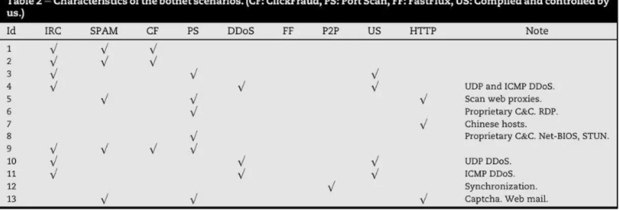
The CTU-13 Dataset is a botnet traffic dataset that was captured in the year 2011 at CTU University located in the Czech Republic. It is a labeled dataset that comprises of botnet, normal and background traffic. The dataset is a mixture of traffic and consists of 13 scenarios where each scene was created with a different malware sample as shown below in Table 1.

Table 1: Dataset Scenario Description

A normal traffic is a traffic that corresponds to traffic created by a naive user like opening mail inbox, surfing social media websites and scouring the internet for online resources [18]. On the other hand, background traffic is the traffic that is generated to obscure the presence of botnet traffic. As described previously, every attack scenario was captured in a pcap (packet capture) file

18

that involved all the three variants of the traffic. The pcap file was processed to obtain bidirectional NetFlow files which are labeled and differentiate well between client and server. Much of the work is done on scenarios 1 and the plan is to extend the model to all the remaining 12 scenarios. The scenarios captured have a wide imbalance in the dataset as seen in Table 2.

Table 2: Dataset Diversity Distribution

Scenario Background Flows (%) Botnet Flows (%) Normal Flows (%) Total Flows

1 97.47 1.41 1.07 2,824,636 2 98.33 1.15 0.5 1,808,122 3 96.94 0.561 2.48 4,710,638 4 97.58 0.154 2.25 1,121,076 5 95.7 1.68 3.6 129,832 6 97.83 0.82 1.34 558,919 7 98.47 1.5 1.47 114,077 8 97.32 2.57 2.46 2,954,230 9 91.7 6.68 1.57 2,753,884 10 90.67 8.112 1.2 1,309,791 11 89.85 7.602 2.53 107,251 12 96.99 0.657 2.34 325,471 13 96.26 2.07 1.65 1,925,149 B. Dataset Features

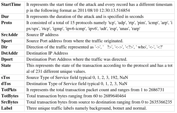
The CTU-13 dataset scenarios have a total of 15 columns namely ‘StartTime’, ‘Dur’, ‘Proto’, ‘SrcAddr’, ‘Sport’, ‘Dir’, ‘DstAddr’, ‘Dport’, ‘State’, ‘sTos’, ‘dTos’, ‘TotPkts’, ‘TotBytes’, ‘SrcBytes’, and ‘Label’. The description of each column is shown in Table 3. The direction field identifies the TCP connection source and the center character represents the transaction state. For the direction column, it includes various symbols like ‘-’, ‘|’, ‘o’, ‘?’. The symbol ‘-’ means the transaction was normal, ‘|’ means the transaction was RESET, ‘o’ means the transaction timed out and ‘?’ means that the transaction direction was unknown. Each dataset of various scenarios has a different distribution of the traffic and it means that it is widely imbalanced.

19

Table 3: Feature Columns Description

StartTime It represents the start time of the attack and every record has a different timestam p in the following format as 2011/08/10 12:30:13.516854

Dur It represents the duration of the attack and is specified in seconds

Proto It consisted of a total of 15 protocols namely 'tcp', 'udp', 'rtp', 'pim', 'icmp', 'arp', 'i px/spx', 'rtcp', 'igmp', 'ipv6-icmp', 'ipv6', 'udt', 'esp', 'unas', 'rarp'

SrcAddr Source IP address

Sport Source Port address from where the traffic originated.

Dir Direction of the traffic represented as '->', ' ?>', '<->', '<?>', ' who', '<-', '<?'

DstAddr Destination IP Address

Dport Destination Port Address where the traffic was directed.

State This represents the state of the transaction according to the protocol and has a tot al of 231 different unique values.

sTos Source Type of Service field typical 0, 1, 2, 3, 192, NaN

dTos Destination Type of Service field typical 0, 1, 2, 3, NaN

TotPkts It represents the total transaction packet count and ranges from 1 to 2686731

TotBytes Total transaction bytes ranging from 60 to 2689640464

SrcBytes Total transaction bytes from source to destination ranging from 0 to 2635366235

Label Three unique traffic labels namely background, botnet and normal.

C. Descriptive Analytics

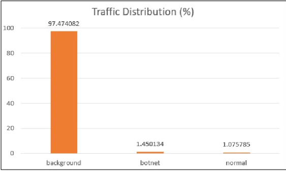
CTU-13 dataset scenario 1 has total records of 2824636 records out of which 97.5 % traffic is the background traffic, botnet traffic is 1.5 % and normal traffic is 1 %. The distribution of traffic is shown in Figure 2 and it shows a wide imbalance that is present in the dataset. Protocol feature has 80.4% traffic using UDP protocol, followed by 18% of TCP protocol and remaining others. The distribution of protocol is shown in Figure 3. The direction of the traffic was mainly bi-directional of 77.6 % followed by from source to destination with 21.8%. 99.9% of traffic utilized ‘sTos’ value of 0 and almost 100% of traffic used 0 value for dTos.

20

Figure 2: Traffic Frequency Distribution

21

VI. PREPROCESSING

CTU-13 Dataset contains an integer, float, object and categorical columns. Columns like Start Time, Source and destination IP address, and source and destination port have a large cardinality, and columns like sTos and dTos have a very low cardinality. In order to address these issues, pre-processing needs to be done on the CTU-13 dataset to make it compatible with machine learning training and prediction.

A. One Hot Encoding

A categorical column is a column that comprises of categories and the cardinality is minimal in nature. In CTU-13 Dataset there are 4 columns identified as categorical columns namely ‘Dir’, ‘Proto’, ‘sTos’ and ‘dTos’. ‘Dir’ column has 7 categories, ‘Proto’ has 15 categories, ‘sTos’ column has 6 categories and ‘dTos’ has 5 categories. One Hot encoding refers to the process of converting categorical columns into vectors of 0’s and 1’s. A column having 2 and 3 classes will have a vector length of 2 and 3, respectively. Converting a categorical column of 5 classes into a vector of 0’s and 1’s of length 5 gives rise to the issues of multicollinearity. The problem of multicollinearity results in supplying redundant information and having highly correlated predictors. The issues can be solved by dropping one of the one-hot encoded classes of a column. So, a column with 5 categories will have a vector of length 4 instead of 5. In the case of CTU-13, the number of one-hot encoded columns for 4 categorical columns will be now 29 columns.

B. Label Encoding

The target column in CTU-13 Dataset is the Label column. The Label column can be categorized into three classes namely background, botnet and normal. For any machine learning model to work properly, it is required to have all the predictor variables and response variables to be numeric. In order to do so, the Label columns need to be converted into numbers. Label

22

Encoding refers to the process of assigning labels to those string categories starting with 0. In the case of CTU-13 Dataset, background, botnet, and normal labels were mapped into 0, 1 and 2 respectively. Again, the distribution of those labels was imbalanced as discussed in Section V.C. C. Dropping Columns

Columns with very high cardinality and columns that cannot be converted into any numeric values can be dropped. In CTU-13 Dataset, columns like ‘StartTime’, ‘SrcAddr’, ‘Sport’, ‘DstAddr’, ‘Dport’ and ‘State’ were dropped to reduce some of the features in the dataset.

D. Scaling

Machine learning models often suffer from the problem of calculation done on big numbers as the amount of calculation going under the hood is enormous. If not properly taken care of, this may result in a memory leak, increased training time, slower prediction time, and it will not scale well if the number of features presented to the model increases. An initial run of the baseline model on not-scaled values resulted in the termination of the model training due to the memory resource exhaustion. To handle such cases, it is necessary that such values be scaled to align in a range. Such issues generally happen with a column that has many values and where the range is large. Table 4 show the range of 4 such columns from the CTU-13 dataset. The columns specified were scaled to lie in the range of 0 and 1.

Table 4: Continuous Features Statistics

Column Min Value Max Value Unique Count

Dur (in secs) 0.0 3600.031006 1073189

TotPkts (count) 1 2686731 3548

TotBytes (count) 60 2689640464 69949

23

VII. FEATURE SELECTION

The number of features present in the initial CTU-13 dataset was 15 features. After performing one-hot encoding and dropping of irrelevant columns which basically affects the dataset, the number of columns increased from 15 to 32. Training a machine learning model directly on all the 32 columns might not give the best results. Fundamentally, there are three problems associated with having a multitude of columns: machine learning model training time increases, redundant memory resource allocation, and multiple features often tend to confuse the model. The world of machine learning often suffers from the problem of the curse of dimensionality, and a garbage input to the model will always give garbage output. To deal with such issues of dimensionality, feature selection, also called attribute selection or variable selection, is taken into consideration. The following subsections give a deep dive into feature selection techniques that were considered for obtaining optimal results.

A. Removing Null Columns

The simplest and easiest way of getting rid of redundant columns is by dropping columns that have many null values. In the case of the CTU-13 dataset, the columns exhibiting null values were ‘Sport’, ‘Dport’, ‘State’, ‘sTos’ and ‘dTos’. Columns namely ‘Sport’, ‘Dport’ and ‘State’ were dropped because of their nature that they could not be converted to numeric values. ‘sTos’ and ‘dTos’ were median imputed for the null values. In the CTU-13 dataset, null values were found in ‘Sport’, ‘Dport’, ‘State’, ‘sTos’ and ‘dTos’ columns. Apparently, ‘Sport’, ‘Dport’ and ‘State’ were dropped. ‘sTos’ column null values were imputed with mode value of the column which was 0.0. ‘dTos’ column as seen in the next variance thresholding section was dropped.

24 B. Variance Thresholding

The concept of variance thresholding stems from the fact that the columns that have the same value or little difference in values do not contribute to response prediction. Technically as suggested in [19], a column with low variance or zero variance can be discarded. The default behavior of variance thresholding function from the sklearn library is to keep columns with non-zero variance. For the CTU-13 dataset, a threshold of 0.9 was given to discard columns exhibiting variance less than that which resulted in a significant reduction of feature columns. All the columns of the CTU-13 dataset displayed some range of variance ranging from 0 to 1. The only column that displayed close to zero variance was the ‘dTos’ column as 99.5% of the data belonged to one value and remaining to other values as shown in Figure 4.

Figure 4: Variance Thresholding

C. Filter Methods

Filter methods are also called a univariate selection technique and it refers to the process of performing statistical tests on each individual feature column with the target column independently. The columns exhibiting statistical significance are kept for model training and testing. From [20], it has been suggested that if the input column is numerical and the response column is categorical, the statistical test that should be considered is ANOVA (analysis of

25

variance). If the input column is categorical, then Chi-Squared should be considered. The process of filter methods helps to identify all features that satisfy a test which can be fed to a model for performance evaluation. Figure 5 gives a pictorial representation of filter method modeling.

Figure 5: Flow Diagram for Filter Methods

For the CTU-13 dataset, the tests under consideration are ANOVA and Chi-Squared. ANOVA is used for comparison of the mean of two or more different groups. It is well suitable for hypothesis testing. The null hypothesis would be all means are the same i.e. 𝐻0: 𝜇1 = 𝜇1 = 𝜇2 =

𝜇₃ = 𝜇_𝑐 which means that all population means are equal. The alternate hypothesis will be that not all population means are the same. For ANOVA, generally, F-test is done since the F-test tests the hypothesis that two variances are equal. An F-distribution is given by 𝐹 = 𝜎𝐵𝑒𝑡𝑤𝑒𝑒𝑛2

𝜎_{𝑊𝑖𝑡ℎ𝑖𝑛}2 which is a

ratio of between-group variance and within-group variance a value close to 1 represents that variance exists. Variance means spread around the means. Calculating F will give a value that corresponds to a p-value, and if it is less than the confidence interval critical values, the hypothesis is rejected suggesting that the variance exists. On the other hand, a Chi-squared test is a way to compare collected data if variation exists in the data by chance or it exists between the variables. Expression of chi-squared values is 𝑋_𝑐2 = ∑(𝑂𝑖−𝐸𝑖)2

𝐸𝑖 where 𝑂𝑖 is the observed value and 𝐸𝑖 is the

expected value. For example, if a coin is flipped 50 times, the head comes up 22 times and tail come up 28 times. A chi-squared test also uses a null hypothesis to validate this chance of variance. It uses a degree of freedom, i.e. 𝑘 (𝑛𝑢𝑚𝑏𝑒𝑟 𝑜𝑓 𝑜𝑢𝑡𝑐𝑜𝑚𝑒𝑠) − 1 and critical values. Using these

26

values, the value of the Chi-Square test can be used to determine if the null hypothesis is rejected or not, and thus if variance exists or not.

[21] says that ANOVA F-test is well suited if the features are quantitative and Chi-squared tests if the features are categorical. The sklearn library provides the implementation of ANOVA as f_classif and Chi-Squared as chi2 in the feature_selection package. Both functions automate the process of statistical test calculation for sample input, namely X(train) and y(target). In order to retrieve the best features from individual statistical tests, the scikit-learn library provides filter methods that return top K features from all features using the SelectKBest method. The method inputs the scoring function and k for top feature and returns (scores, p values) as an array. ANOVA and Chi-Squared both ranked the following features in top 10 i.e. ‘Dur’, ‘Proto_tcp’, ‘Dir_ <->’, ‘Proto_udp’, ‘Proto_icmp’, ‘Dir_ <-‘, ‘Dir_ <?>’, ‘Dir_ ?>’, ‘Proto_rtp’, and ‘Proto_rtcp’. D. Wrapper Methods

Filter methods as described above not take into consideration the interaction with individual columns. On the other hand, wrapper methods take a subset of features and compares them with other combinations of the subset. Such a selection of features can take any type of heuristics like the forward feature selection and backward feature selection for addition and removal of features. Forward feature selection starts with one feature followed by evaluation, and then more features are added to see if the performance drops or not. Features causing a drop in performance are dropped and the process is continued until all the features are tested to obtain the optimal feature set. In the case of backward feature selection, the process is opposite as it starts with all the feature columns and keeps on adding or removing features to obtain optimal performance. A typical wrapper method process is as shown in Figure 6.

27

Figure 6: Flow Diagram for Wrapper Methods

The widely used wrapper method is RFE (Recursive feature elimination) technique. This technique is an optimization algorithm and a greedy one as it tries to find the best feature subset. Initially, it starts with all the features and computes the score that can be obtained using coef_ attribute or feature importance attribute. It discards the lowest-performing feature and continues the process until the desired number of k features is obtained. At every step, it takes a subset of features and creates the model and keeps the best or worst performing feature and continues to do so until all features are used up. In the end, features are returned based on the order they were eliminated. The sklearn library feature_selection package has RFE() that takes an estimator and number of features to select and return the feature set. RFE did a pretty good job of estimating the features that were later selected for model training but suffered from time complexity issues as it had to train the model repeatedly to get the top-performing features.

E. Embedded Methods

The filter method might fail to generate the best set of the feature while the wrapper method always does. Also, the filter method is fast as compared to wrapper methods. Embedded Methods comes with the capability of filter and wrapper method qualities. Generally, embedded method based models have their own feature selection methods as shown in Figure 7. Lasso and Ridge-based regression model that employs L1 and L2 penalty regularization are widely implemented

28

for the embedded model. Also, some tree-based classifiers do support the in-built feature selection technique. Sklearn library has SelectFromModel() method that takes in estimators like Lasso and Ridge Regression or Tree Classifiers and returns the features based on classifier feature_importance attribute. Embedded methods tend to be expensive and can be shown visualized in the below diagram. SelectFromModel() using Random Forest recommended only using ‘Dur’, ‘TotPkts, ‘TotBytes’, ‘SrcBytes’ and in some cases only ‘Dur’ and ‘TotPkts’ without a drop in performance.

Figure 7: Flow Diagram for Embedded Methods

F. Feature importance and Correlation Heatmap

Feature importance is applicable to any machine learning model that has the feature_importance as a parameter. The correlation coefficient involves understanding correlation. A covariance gives a nice description of how to feature vary with each other. Mathematical expression for covariance between feature 𝑥 and 𝑦 is given by 𝜎_𝑥𝑦 = ∑(𝑥−𝑥̅)(𝑦−𝑦̅)

𝑁 where 𝑥̅ and 𝑦̅

are the mean of the x and y feature. The correlation coefficient is given by 𝜌𝑥𝑦= 𝜎𝑥𝑦

𝜎𝑥𝜎𝑦 where 𝜎𝑥

and 𝜎_𝑦 are the variance of 𝑥 and 𝑦 respectively. Also, the correlation matrix depicts the correlation between each input feature which ranges from -1 to +1. A value of 0 means there is no correlation and otherwise, a correlation exists. For features that are highly correlated with each other, one of the features can be dropped from the final feature selection set.

29

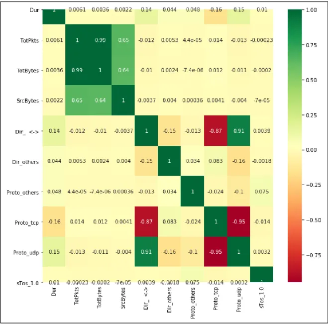
The correlation matrix in Figure 8 indicates that the columns ‘TotBytes’ and ‘Totpkts’ are highly correlated with a value of 0.99. Similarly, ‘SrcBytes’ is positively correlated with ‘TotPkts’ and ‘TotBytes’. Negatively correlated columns are ‘Proto_tcp’ and ‘Dir_ <->’. Also, by making use of ExtraTressClassifier which internally uses decision Tree for feature importance resulted in the selection of ‘Dur’, ‘TotPkts’, ‘TotBytes’, ‘SrcBytes’, ‘Dir_ <->’, ‘Dir_others’, ‘Proto_others’, ‘Proto_tcp’, ‘Proto_udp’ and ‘sTos_1.0’ columns.

30

VIII. ADDRESSING DATA IMBALANCE

As described previously, the CTU-13 dataset has an imbalance issue. Generally, the imbalance issues are in the ration of 8:2 or 9:1 but in the CTU-13 dataset case, the imbalance is extreme. Botnet traffic is just 1.5% of the entire network traffic where a majority of 97.5% of traffic is background traffic. A critical task is to have a model that generalizes well to the minority class. Machine learning models are inclined to learn the majority class features and tend to overfit the training dataset. The accuracy obtained represents the majority class. In the CTU-13 dataset, the accuracy obtained over the baseline model is 97.5% which is the same as the majority class proportion. In order to address these, some techniques have been suggested in the literature to overcome imbalance and extreme imbalance issues.

A. Undersampling

When the number of majority class samples are very high in comparison, under-sampling can be used to reduce the number of samples from the majority class to make it equal to minority classes as shown in Figure 9. It removes some of the observations from the majority class which could result in underfitting as it may be representative of minority class and not majority class. The imblearn.under_sampling package provides RandomUnderSampler() function to perform under sampling on the majority class. This function balances the dataset by randomly choosing a subset of data for the targeted class. RandomUnderSampler() is a controlled undersampling technique. It also provides a facility to choose samples with or without replacement. This allows us to specify the number of samples and falls under the category of controlled under-sampling. There is another category of cleaning under-sampling technique that makes use of heuristics to clean the dataset without specifying the number of samples for each class called as Tomek’s links [22-24].

31

Figure 9: Illustration of Undersampling [22] Figure 10: Illustration of Undersampling - Tomek Links [23]

In RandomUnderSampling(), the samples from the majority class are removed randomly without any consideration of the underlying distribution. The NearMiss algorithm mentioned in [22] for undersampling uses a heuristic to clean the dataset and it has three variants of doing so in selecting the data points from the majority class. Tomek links are widely popular for undersampling as it works on a set of rules. [23] says that two samples have a Tomek’s link if they are the nearest neighbors of each other and they are apparently deleted from the dataset space. A nice general rule for the identification of two samples from x and y class is defined such that for a sample z, it satisfies the equation 𝑑(𝑥, 𝑦) < 𝑑(𝑥, 𝑧) 𝑎𝑛𝑑 𝑑(𝑥, 𝑦) < 𝑑(𝑦, 𝑧) and is shown in Figure 10. The edited nearest neighbor (ENN) makes use of the nearest neighbor algorithm and removes samples that do not agree with the nearest neighbor algorithm [24].

B. Oversampling

This method is the exact opposite of Undersampling. First one is the naïve random oversampling provided in imblearn.over_sampling package RandomOverSampler function(). It generates a new sample for minority class by simply creating samples with replacement from minority class as depicted in Figure 11. This strategy of increasing the samples might bloat the

32

performance of the model, increase the training time and get complacent with the same minority class sample. Apart from replacement oversampling, there are two other techniques namely SMOTE (Synthetic Minority Oversampling Technique) as shown in Figure 12 and ADASYN (Adaptive Synthetic) can be used to resample minority class.

Figure 11: Illustration of Oversampling [22] Figure 12: Illustration of SMOTE [26]

RandomOverSampler randomly creates duplicates of minority samples to achieve a balanced dataset. To overcome overfitting, [25, 26] proposes a technique of generating synthetic samples using SMOTE and ADASYN. SMOTE identifies two nearest neighbor samples and calculates the difference in the feature vector followed by multiplication with a random number to create a new feature vector or sample. All the new feature samples fall in between the respective two nearby samples. This is different in the case of ADASYN, where [26] employs the creation of a new sample by adding some variance so that it is better scattered among the minority samples.

C. Oversampling followed by Undersampling

SMOTE, which is an oversampling method, generated a noisy sample which can affect the model performance. It is necessary to clean the space resulting from over-sampling by employing undersampling techniques, namely Tomek’s link and edited nearest neighbor (ENN) technique. The imblearn.combine provides two functions SMOTETomek and SMOTEENN that combines

33

the features of oversampling followed by undersampling. [27] presents a brief account of how oversampling followed by undersampling can solve some issues of space cleaning. However, there is a tradeoff with performance as the time complexity increases by applying the nearest neighbor algorithm twice. In the strategy3 dataset, the time complexity has increased, and it does not scale well to increasing dataset size, and the prediction accuracy was not good enough to consider it for future enhancements.

D. Ensemble Learning

Instead of having a single learner, it is better to have an ensemble of learners trying to learn the same thing, and this technique generalizes well to the majority and minority class. In this section, the working of ensemble learning is explained in detail.

A bagging classifier is an ensemble that trains the base classifiers on the random subsets of the original dataset followed by aggregating their prediction to get a final prediction. In this case, the base estimator is the decision tree. However, a bagging classifier does not handle the imbalance scenarios. In order to do so [28] specifies that a balanced bagging classifier handles the imbalance while at the same time doing ensemble learning, and it is found to deliver better results than single learners. The behavior of the model can be controlled by fine-tuning the sampling strategy and the replacement criteria. On the same line, the random forest classifier and balanced random forest classifier has the same behavior as bagging classifier and balanced bagging classifier, respectively. The easy ensemble is a technique of bagging boosted learners. Boosted learner typically starts with a set of weak learners and chooses the best learners and iteratively continues to do so until a stopping criterion is met. EasyEnsemble classifier makes use of base estimators like AdaBoost and bags AdaBoost learners who are trained on balanced samples. RusBoostClassifier randomly undersamples the available dataset followed by iteratively performing boosted learning.

34 E. Cost-Sensitive Learning - XGBoost

Machine learning models are generally cost insensitive at the time of training meaning that they do not consider the classification error made during training. While most of the models do have fine-tuning parameters to support this, it is limited in its own way. XGBoost model is built to work on an imbalanced dataset because it is robust to survive data imbalance since the resampling occurs internally [30]. XGBoost is called extreme gradient boosting and is a sequential decision tree as shown in Figure 13.

Figure 13: XGBoost Model

Initially, all the feature vectors have equal weights to increase the likelihood of being selected for building the first decision tree classifier. The first tree classifier does its prediction and increases the weight for every wrong classification done using the feature. Since the first classifier was unable to do the correct classification, it is labeled as a weak classifier. The next classifier will take the updated weights and re-train them. This process will continue until the last decision tree classifier is built. In the end, the final classifier takes a vote among the weak learners to get the final prediction. XGBoost algorithm has an inbuilt train and predict method and is available through xgboost python package. The scikit-learn library has a wrapper on the top of the xgboost called XGBClassifier to achieve the same purpose.

35

IX. MACHINE LEARNING CLASSIFIERS

A wide array of machine learning models is suitable for classification stack. For this project, most of the topics focus on the decision tree, random forest and AdaBoost classifier.

A. Decision Tree

A decision tree classification is made based on the mode of the class and used when the dependent variable is categorical. The decision tree continues to grow until a stopping criterion is reached. A full-grown decision tree is bound to overfit as it will not be able to handle the unforeseen data. The Decision Tree works by identifying the features, selecting the condition for splitting and the stopping criteria followed by pruning the overgrown branches. The decision split is made using the Gini index, chi-square value, information gain or reduction in the variance. Figure 14 represents a typical decision tree model.

Figure 14: Illustration of Decision Tree

B. Random Forest

A Random Forest is a forest of decision trees that makes it more robust and delivers higher accuracy. The process of random forest starts with taking a subset of samples from the training set of size N followed by taking m input features from a total of M features and then the decision tree is built to the largest extent possible without pruning. Finally, the output is predicted by taking majority votes from the individual trees. Random Forest is a bagging model, does not overfit and

36

works well for a dataset with large dimensionality. A pictorial representation of the random forest is shown in Figure 15.

Figure 15: Illustration of Random Forest

C. AdaBoost

An AdaBoost (Adaptive Boosting) is a forest of trees where trees have a root node and two children, and they are called stumps. Stumps are weak learners and AdaBoost combines the weak learners to make the classification. Also, some of the stumps get more say in the classification than others. Every other stump in the iteration is made by taking previous stumps into account. AdaBoost starts by creating a stump for each feature column with an initial equal weight. Then it calculates the accuracy and based on that the weights are decreased or increased when the classification is wrong. Figure 16 highlights the AdaBoost process.

37

X. TECHNOLOGY STACK

A. Hardware

The models built were trained on a Windows 10 workstation and on Google Cloud. 1) Workstation:

a. Processor: Intel® Core ™ i7-8750H CPU @2.20GHz 2.21 GHz b. RAM: 16.0 GB

c. System Type: 64-bit OS, x-64 based processor 2) Google Cloud:

a. Processor: Python 3 Google Compute Engine Backend b. RAM: 13.0 GB

B. Software and Libraries

1) Jupyter Notebook: It is an open-source application that facilitates data preprocessing, statistical modeling, data visualization, machine learning and much more.

2) Google Colab: It is a colab notebook hosted on google cloud servers providing access to GPU’s and TPU’s for tasks that can be done in a Jupyter notebook

3) Libraries: Python was used as the scripting language for writing most of the code.

a. Scikit-learn: It is used for predictive analytics tasks like classification, regression, clustering, dimensionality reduction, model selection and preprocessing.

b. Imblearn: This library provides an API for imbalanced learning and wide samples. c. Xgboost: It is a highly efficient gradient boosting library for xgboost classifiers. d. Pandas: It is a data analysis and manipulation library implemented in python e. NumPy: It provides numerical computing capability and high-level mathematical

functions for multidimensional arrays and matrices.