Titre:
Title
: Tracing and profiling machine learning dataflow applications on GPU
Auteurs:
Authors
: Pierre Zins et Michel R. Dagenais
Date:
2019
Type:
Article de revue / Journal articleRéférence:
Citation
:
Zins, P. & Dagenais, M. R. (2019). Tracing and profiling machine learning dataflow applications on GPU. International Journal of Parallel Programming, 47(5-6), p. 973-1013. doi:10.1007/s10766-019-00630-5
Document en libre accès dans PolyPublie
Open Access document in PolyPublie
URL de PolyPublie:
PolyPublie URL: https://publications.polymtl.ca/4213/
Version: Version finale avant publication / Accepted versionRévisé par les pairs / Refereed Conditions d’utilisation:
Terms of Use: Tous droits réservés / All rights reserved
Document publié chez l’éditeur officiel
Document issued by the official publisher
Titre de la revue:
Journal Title: International Journal of Parallel Programming (vol. 47, no 5-6)
Maison d’édition:
Publisher: Springer
URL officiel:
Official URL: https://doi.org/10.1007/s10766-019-00630-5
Mention légale:
Legal notice:
This is a post-peer-review, pre-copyedit version of an article published in International Journal of Parallel Programming. The final authenticated version is available online at:
https://doi.org/10.1007/s10766-019-00630-5
Ce fichier a été téléchargé à partir de PolyPublie, le dépôt institutionnel de Polytechnique Montréal
This file has been downloaded from PolyPublie, the institutional repository of Polytechnique Montréal
Tracing and profiling machine learning dataflow applications on GPU
Pierre Zins
Ecole Polytechnique Montral
Montreal, Quebec H3T 1J4
Michel R. Dagenais
Ecole Polytechnique Montral
Montreal, Quebec H3T 1J4
[email protected]Abstract— In this paper, we propose a profiling and trac-ing method for dataflow applications with GPU acceleration. Dataflow models can be represented by graphs and are widely used in many domains like signal processing or machine learning. Within the graph, the data flows along the edges, and the nodes correspond to the computing units that process the data. To accelerate the execution, some co-processing units, like GPUs, are often used for computing intensive nodes. The work in this paper aims at providing useful information about the execution of the dataflow graph on the available hardware, in order to understand and possibly improve the performance. The collected traces include low level information about the CPU, from the Linux Kernel, as well as high-level information about the dataflow model. This is followed by post-mortem analysis and visualization steps in order to enhance the trace and show useful information to the user. To demonstrate the effectiveness of the method, it was evaluated for TensorFlow, a well-known machine learning library that uses a dataflow computational graph to represent the algorithms. We present a few examples of machine learning applications that can be optimized with the help of the information provided by our proposed method.
I. INTRODUCTION
Achieving very high performance is an essential aspect of computing systems. The improvement in traditional CPU performance has recently slowed down. Indeed, techniques used to improve the performance like increasing the CPU clock frequency and adding more memory cache have reached a limit. Therefore, newer improvements largely consist in using highly parallel computing environments to achieve better performance. Heterogeneous architectures have emerged, in which traditional CPUs get support from co-processing units like GPUs, FPGAs or DSPs. With the appearance of General Purpose GPU (GPGPU), GPUs are no longer only intended for graphical applications [1]. They are increasingly used for general purpose computations. In order to benefit from these new parallel architectures, the dataflow model has become very popular. It is a data-centric model and can be represented as a graph, where nodes are the operations that are applied to the incoming data, and edges represent the flow of data. It is used in different domains like signal processing [2], [3], [4], [5] and image [6] or video processing [7]. New languages based on this approach have also been developed [8], [9], [10] and [11]. They are inherently parallel and therefore well adapted to heterogeneous platforms. In the machine learning domain, Krizhevsky, Sutskever and Hinton [12] demonstrated the advantages of using GPUs to implement
deep learning models for images. Consequently, the dataflow model became popular in this field as well and libraries like Theano [13], [14] and TensorFlow [15], [16], [17] use it to jointly program the CPU and GPU. In order to insure maximum performance, we need to be able to analyze the execution of the dataflow application. The challenge here is to evaluate the execution on all the available hardware and insure that we maximize their usage.
Tracing and profiling are two techniques that can help to identify several types of problems, like deadlocks, bugs, bottlenecks or inefficient hardware usage. Applying them to the CPUs cores, either on the kernel side or the user side, is a task already well explored and has demonstrated its efficiency in the past [18] and [19]. However, in the case of heterogeneous architectures, it is not sufficient, as we also need to collect information about the co-processing units used.
In this work, we focus on the case where the CPU gets support from a GPU. Profiling a GPU is usually possible thanks to GPU vendors tools like CodeXL for AMD, Nsight for Nvidia and Graphic Performance Analyzer for Intel. They target specifically the GPU and do not provide information about the CPU. For that, the integration with an external element or method is necessary but seems difficult, because the internal characteristics of these tools are not documented or published. The offered visualizations are also specifically defined and cannot be modified. Moreover, it is not possible to develop new views according to the user needs. Furthermore, each tool is limited to the hardware of a specific vendor. Therefore, it is not possible to achieve a general solution based on one of these tools that can work with GPUs from different vendors. Finally, the goal of profiling and tracing dataflow applications is to propose a unified view, gathering information from every device, as well as developing specialized views focused on some key points like the memory consumption or the memory transfers between the devices. The flexibility required for that purpose is not available in the tools proposed by the GPU vendors.
In this work, we evaluated our method with Tensor-Flow. This library uses an efficient dataflow approach and is designed for heterogeneous architectures, and GPUs in particular. The choice was also motivated by its very high performance and popularity in the machine learning domain. In this paper, we propose a profiling and tracing method
for dataflow applications that use a GPU. Several elements are analyzed and we obtain, as a result, a detailed trace of the execution of the dataflow application. We maintain a very low overhead, to minimize the impact on the studied application. We developed appropriate views and analyses that are highly beneficial for users.
The originality of our work resides in the combination of information from several layers and from all the computing units involved. In our approach, we combine low-level in-formation related to the Operating System or the GPU, with mid-level information from several libraries, and high-level knowledge about the dataflow model. As a result, we obtain a trace containing a rich set of events. Different analyses and visualizations allow users to obtain useful information in order to guide their optimization efforts.
The paper is organized as follows. First, we describe existing work in the domain of CPU, GPU and dataflow systems tracing and profiling. Then, we explain the different parts of the method. In section 3, we apply our method to different TensorFlow applications. We show in particular how the views obtained can help a user to understand the performance and suggest optimizations. After that, we evaluate the proposed method for TensorFlow by computing its overhead on different platforms. Finally, we conclude and suggest some possible directions for future work.
II. RELATED WORK
The related work section is composed of three subsections. We start by describing existing work on tracing and profiling the CPU. Thereafter, we cover GPU profiling and, finally, we look at existing work about dataflow model analysis. A. CPU tracing and profiling
Tracing is a technique that consists in recording some events during the execution of an application. This process aims to impose a minimal overhead, compared to a normal execution of the application. Obviously, this depends strongly on the number of collected events. Tracing is well-known for performance analysis and several tools have already been developed in this regard. Most of them are intended to work on GNU/Linux. Indeed, tracing often involves a static instrumentation of the source code and, therefore, open-source projects are more suitable. In spite of being more limited, tracing in closed-source environments is also possible, like ETW for Windows. Profiling is another technique for performance analysis and corresponds to the process of gathering some metrics about the execution of an application. For example, monitoring the memory usage of a device, or sampling hardware performance counters refer to profiling. In the next paragraphs, we present the main tools for CPU tracing and profiling.
1) strace: Straceis a Linux tool that can trace all the system calls as well as the signals received by a process. This tool is relatively popular due to its ease of use. Therefore, it is a powerful option for troubleshooting Linux systems and is often chosen by system administrators.
However, its poor performance and the high overhead introduced is a major drawback.
2) Perf and Ftrace: PerfandFtraceare two solutions integrated directly into the Linux Kernel for performance analysis.
WithPerf, the entire system (userspace and kernel space) can be statistically profiled. For example, performance coun-ters from the CPU can be collected. Static instrumentation of the source code and dynamic instrumentation usingkprobes and uprobes, respectively for kernel and userspace tracing, are also available.
Ftrace[20] is a tracing framework for the Linux Kernel and contains several tracers to collect different information. Originally designed for static instrumentation, new features were gradually added, including dynamic tracing of kernel functions using kprobes. Filtering is also available and allows the user to collect only some specific information. Ftrace is managed with a special file system, named TraceFS. 3) LTTng: LTTng is a Linux tool for kernel side and userspace side tracing [21]. Unlike Ftrace and Perf, its kernel tracer module is loaded at the start of the tracing subsystem and is not part of the Linux kernel. LTTng has been developed to support the tracing of multithreaded applications. The overhead introduced is lower than with other tools [?]. Collecting events with LTTng, produces a trace in CTF format (Common Tracer Format). This stan-dardized binary format was developed with the objective of optimizing the trace writing performance and the compact-ness.Babeltraceis the main tool to read and write CTF traces, and Trace Compass offers a flexible visualization and analysis environment. Due to its ease of use and its high-performance multi-level tracing capabilities, we usedLTTng in this work.
B. GPU tracing and profiling
Tracing GPUs consist in two main parts. The first part provides information about the GPU activity but is performed on the CPU. It consists in collecting all the function calls to the GPU libraries like CUDA or OpenCL. This part can be performed by some of the tools described previously. The second part consists in gathering the timestamps of every GPU related event: GPU kernels, memory copies, and synchronization barriers. Profiling the GPU is also possible by collecting performance counters. The latter represent useful metrics that can give insights into the performance of a GPU kernel function executed on a GPU.
1) Nvidia nvprof and Nsight: Nsightis a performance analysis environment developed by Nvidia for their GPUs. It offers debugging but also profiling capabilities with nvprof. The latter can be used insideNsightor directly in a command-line version. A lot of information about the GPU can be collected: CUDA API function calls, the begin-ning and end times of asynchronous events like GPU kernels
or memory copies and performance counters. Nvidia is also going to release shortly three new tools for performance analysis. The first one is a system-wide performance analysis tool calledNsight Systems.Nsight Computeis the second one and focuses on GPU kernels profiling. The last tool is Nsight Graphics and concerns graphics applications.
Nvidia tools present several limitations. First, the results of a profiling session are in a binary and proprietary format that is intended to be used within theNsightenvironment only. Moreover, these tools focus on the analysis of the GPUs, which is insufficient in our context. Finally, the visualizations offered are strictly defined and cannot be modified, extended or improved by users.
2) CodeXL: CodeXLis a suite of profiling tools designed for AMD hardware. LikeNsight, this tool offers profiling and debugging opportunities. It is available as a standalone application on Linux and also as a Visual Studio extension on Windows. CodeXLoffers several features like OpenCL API profiling, APU/CPU/GPU power profiling, performance counters collection and graphics API tracing (OpenGL, Vulkan, and DirectX). Internally, it uses different tools and libraries like RCP (Radeon Compute Profiler) or GPA (GPU Performance API).
Like the Nvidia tools, they target exclusively the GPUs, and the proposed views cannot be modified. Therefore, CodeXL lacks flexibility and it might be difficult for a user to integrate it into a tracing and profiling environment.
C. Dataflow profiling
In the two previous subsections, we described existing tools for tracing and profiling the CPU as well as the GPU. This subsection presents work focused on analyzing dataflow models. Canale et al. [22] described a new method based on Petri nets for optimizing and representing dataflow programs. A heuristic algorithm has also been developed to find an optimal buffer size for data streams. This approach provides a relatively high level analysis of dataflow programs, and they demonstrated its efficiency to optimize well-known stream-ing applications like JPEG or MPEG decodstream-ing. Janneck, Miller and Parlour [23] presented some techniques for ana-lyzing the execution of dataflow programs. They introduced the notion of causation traces, as well as some analysis techniques that can be applied. As for the previous work, they illustrated the benefit of their technique with streaming ap-plications like MPEG-4 decoders. Casale Brunet, Mattavelli and Janneck [24] explained another dataflow trace analysis to optimize signal processing algorithms. The effectiveness of the technique is demonstrated with two examples : MPEG-4 SP and AVC/H.26MPEG-4 video decoders. Mysore et al. [25] developed a data tagging method at ISA level. The latter can be compared to medical techniques that consist in injecting a radioactive substance into a human to detect heart disease, for example. Their work is focused on dataflow systems and allows a user to collect information at different layers, from
the kernel of the operating system up to the applications. However, the introduced overhead is problematic, and the visualization of the results is a challenge because of the amount of information collected. Finally, Osmari et al. [26] described Smart Trace, a trace analysis tool specialized for parallel and especially dataflow traces. The authors presented a set of dataflow-centered visualizations and analyses and showed the efficiency of each.
III. PROPOSED METHOD
In this section, we discuss the concepts and principles of the proposed method. We start with a presentation of TensorFlow. We quickly explain some principles and key elements of this library. We also mention some technical constraints and limitations when using it with a GPU. Then, we continue with a description of the instrumentation of TensorFlow. After this, we present different steps to get information about the GPU activity. Once all the data has been collected, we address the traces post-processing steps. Finally, we present the views and analysis developed to visualize the results.
A. TensorFlow concepts
This research work aims at profiling machine learning dataflow applications that use GPU acceleration. The pro-posed method is general but, in order to apply the work on a concrete example, we decided to use TensorFlow. It is therefore useful to explain some concepts about this library. Developing an application with TensorFlow usually in-volves two distinct steps. First, the user combines several operations to create the computation graph of the model. The second step is just the execution of this graph. When training a model, a backward pass is usually involved in order to up-date the weights of the model. From a dataflow perspective, this pass is not problematic and simply represents additional nodes in the graph. Globally, the training process requires many executions of the model with different data as input.
TensorFlow use a specific object calledSessionto manage the graph. This object offers a method named Runthat can trigger one execution of the graph. From a practical point of view, the user calls many times therunmethod of the unique Sessionobject, each time with new input data. Each call starts one execution of the graph with the provided input data. Thus, the whole training process is composed of a succession of graph executions. Our work mostly targets the training step, as it is the most demanding in terms of computation and duration, but the inference step can also be analyzed just as well. The only difference with the training step is the absence of the backward pass, which has no effect it terms of tracing or profiling.
B. TensorFlow with a GPU
Using TensorFlow with GPUs adds some technical con-straints. Indeed, as the vast majority of machine learning libraries, the official support for GPUs in TensorFlow is done withCUDA, which means that it is only usable with Nvidia hardware. Two main efforts exist in order to support GPUs
from other vendors. They are still in development and not entirely up-to-date with the official version of TensorFlow.
The first possibility concerns AMD GPUs, through ROCm, an open-source platform for GPU-enabled high-performance computing developed by AMD [27]. This platform is based on HSA (Heterogeneous System Architecture) [28], a hard-ware and softhard-ware stack that allows the different computing units, like CPUs or GPUs, to cooperate efficiently. Sev-eral other open-source libraries from AMD are used like HIP (Heterogeneous-Compute Interface for Portability), a CUDA-like single source C++ API for GPU programming, and HC (Heterogeneous Compute), a lower-level C++ API for accelerated GPU computing.
The second option is more general and consists in a new SYCL backend for TensorFlow [29]. SYCL [30] is a specifi-cation from the Khronos Group that provides an abstraction layer on top of OpenCL. It brings several improvements like the support for modern C++ and the single source programming feature. This solution is supposed to work with a wide variety of GPUs and is not limited to AMD or Nvidia GPUs.
Apart from some technical details, the general idea re-mains the same, on all platforms and with the three imple-mentation versions of TensorFlow. In the next subsections, we present the different parts of the proposed method. C. TensorFlow instrumentation
Dataflow applications can usually be seen as a graph composed of nodes that represent operations, and edges on which the data flows. In order to profile efficiently those types of applications, we need to have access to the graph. Therefore, an instrumentation of the library that implements the dataflow model is necessary. In this paper we evaluate our method with TensorFlow. Therefore we describe different key parts of it but the general idea of the instrumentation can easily be ported to other libraries.
From a technical point of view, we opted for LTTng for its efficiency and flexibility. Moreover, the resulting trace is in the binary Common Trace Format (CTF) which aims at high performance, especially for writing the trace. When tracing an application, events are recorded each time an LTTng tracepoint is hit. Therefore, the instrumentation is essential and the tracepoints should be inserted carefully at strategic locations in the source code of TensorFlow. We discuss the main elements that should be profiled in the case of a dataflow application.
1) Session: In a dataflow application, the execution con-sists in feeding some data to the input nodes of the graph which triggers the execution of every node in the graph until the output nodes. Every time a node has received all its inputs, it can start computing. Feeding data to the graph, and then retrieving the final results, can be considered as one iteration. Since in a dataflow application new data is continuously fed to the graph, it is necessary to have a general insight of the current state of the dataflow model. Knowing the beginning and the end of every iteration is therefore essential. In TensorFlow, an iteration corresponds
to one call to the Run function of the Session object, as described in subsection III-A. Therefore, our instrumentation deals with these two elements.
2) Operations: In order to profile dataflow applications, we need to trace the different operations that process the data flow. Indeed, they define the behavior of the application. One operation, represented by a node in the graph, performs the same processing continuously on the incoming data. Four main informations should be collected about operations:
1) the processing beginning time 2) the processing end time
3) the device to which the operation is assigned. In this work, two options are possible, either the CPU or the GPU.
4) the type of the operation: synchronous or asyn-chronous.
Usually, most of the computation nodes are assigned to the GPU, because of its higher computation capabilities. In this case, little work is executed on the CPU: preparing the execution with data transfers for example and sending work to the GPU. All the computation happens on the GPU and therefore this component should constitute a priority in the profiling process. The internal instrumentation of the GPU access library is not sufficient to collect the real execution times of the operations executed on the GPU, and this issue is discussed in subsection III-E.
3) Scheduling: In order to understand the behavior of a dataflow execution, it can be interesting to have an insight into how all the operations in the graph are scheduled. Indeed, in many cases, including TensorFlow, several nodes are assigned to the same computing unit and can be ready at the same time. It is therefore important to know how the library decides which node to execute.
Collecting all the beginning and end timestamps of every operation in the graph already brings some information about the scheduling, but we can go deeper. To do that, we need to understand the inner working of TensorFlow, and especially how it schedules the nodes. This part is totally dependent on the library used to implement dataflow applications.
The TensorFlow scheduling mechanism uses a threadpool and two different types of queues: ready and inline ready. When a node finished its execution, the result is available and the successors of the node in the graph are activated. When a new node is ready, it is first enqueued into the readyqueue and TensorFlow continuously schedules the nodes from it. Two options are possible. If the node selected from this queue is expensive, it is dispatched to the thread-pool in a new thread to be executed. Otherwise, the node is considered as inexpensive and is put into the inline ready queue to be executed directly within the current thread. TensorFlow usually considers nodes executed on the GPU as inexpensive, because they consume very few resources on the CPU where the scheduler runs.
In terms of instrumentation, it represents three elements. First, we want to know the nodes scheduled from theready queue. Secondly, we would like to follow all the operations executed from the inline ready queue. Finally, it can be
interesting to know which nodes are activated by each completed node.
4) Memory: The data-centric characteristic of a dataflow model makes memory usage another essential aspect. In this model, data is continuously fed to the graph and flows along the graph edges. As a result, we need to have information about memory usage. This is even more crucial in the case of machine learning applications in which the data considered is usually tensors (multidimensional matrices) that can be very large. It is important to have information about this for the CPU cores, but even more for the GPUs as their memory is a relatively scarce resource, typically much smaller than the CPU RAM. Two elements are analyzed :
• Memory allocations and deallocations • Memory transfers between the devices
In order to use a GPU, a developer generally needs platforms, libraries or frameworks like CUDA or OpenCL. All of them provide some API functions in order to program the GPU. In particular, a few functions offer the possibility to allocate memory on the host (CPU) or on the device (GPU) and to transfer data between them. The idea here is to locate all the calls to these specific functions in the analyzed application and to instrument them. If the application provides an internal wrapper around these functions like in TensorFlow, the instrumentation process becomes easier. If we consider memory allocations and deallocations, we usually deal with four different functions :
1) Allocate on the Host 2) Deallocate on the Host 3) Allocate on the Device 4) Deallocate on the Host
Instead of calling these functions very frequently, many applications choose to allocate all the available memory on the device at initialization time. Then, the allocated memory is simply managed by an internal allocator. This depends on the library that implements the dataflow model.
If we consider TensorFlow, it uses an internal allocator called BFC Allocator that implements the Best Fit with Coalescingalgorithm. This allocator is used for every device (CPU or GPU), and simply adds another level of instrumen-tation, as we need to find all the functions related to memory allocation and memory deallocation within this allocator. Inside TensorFlow, the BFC Allocator is a simple version of the Doug Lea’s malloc (dlmalloc) [31] and splits all the memory into several chunks. They represent a memory fragment of a specific size. Moreover, chunks are stored into bins which are collections of similar-size free chunks. This allocator is supposed to keep fragmentation to a minimum. Thus, in order to have a finer-grained analysis of memory management inside TensorFlow, we instrumented this allo-cator. As a result, we can bring three statistics out.
1) Global statistics for the allocator, with several metrics: the number of bytes in use, the number of allocations, the maximum number of bytes in use and the largest allocation.
2) Chunks statistics which monitor the chunks usage.
Several metrics are available: the total number of chunks, the number of used chunks and the number of free chunks. It also follows the number of bytes used and, unlike the global statistics, it can differentiate the number of bytes used and the number of bytes requested. The difference can be explained by the restrictions for the chunk sizes to certain values, which can be bigger than the real allocation request. With that information, we can also compute the number of wasted bytes.
3) Bins statistics: These monitor all the bins by giving the number of chunks in each bin and the corresponding number of bytes.
As mentioned before, memory transfers between devices are also important. When using GPUs, a memory transfer is considered as a command sent to the device to either read or write data. The first case is for memory copy from the Device (GPU) to the Host (CPU) and the second represents a memory copy from the Host (CPU) to the Device (GPU). Moreover, they are usually performed asynchronously by the DMA unit of the GPU, in order to overlap with the computation and consequently hide some latencies. To track them, we collect all the calls to the API functions that cause memory transfers. As for memory allocation, we need to locate all the calls to the corresponding API functions and instrument them. The instrumentation here has two purposes: 1) Getting the duration of the call by adding a tracepoint
just before and just after the call
2) Getting the amount of data involved in the memory transfer
If the memory transfer is performed synchronously, the duration obtained actually corresponds to the time spent to copy the data between the two devices. However, if the copy is asynchronous, the duration only represents the time required to launch a command to the GPU and not the actual duration of the transfer. Getting the real duration of the memory transfers is addressed in section III-E.
5) GRPC: In this work, we focused on dataflow models executed on a single machine. However, it is also possible to distribute the execution on several machines. In this case, the graph is partitioned on several hosts. In addition, each host is free to offer a GPU to accelerate the execution of certain dataflow nodes. Profiling distributed dataflow models is possible with local profiling on each machine, and the pos-sibility to jointly visualize the traces from several machines. In order to enhance the information and to highlight some key points, we also instrumented the code that allows the dataflow models to be distributed on several machines. In the case of TensorFlow, the implementation is based on two elements: gRPC, an open-source and high performance RPC framework, and protocol buffers, a serializing tool to encode the data exchanged over the network. During the execution, if two connected nodes are assigned to two different machines, a tensor request is sent by one machine and the second machine computes the tensor and sends the response back to the first machine.
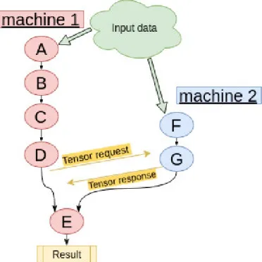
Figure 1 presents an example of a graph with 7 nodes shared among two machines. The first machine can process all the nodes until node E, as they do not require any external element. However, to compute node E, the first machine needs the output of node G which is assigned to the second machine. Therefore, to continue the execution, machine 1 sends a tensor request to machine 2. Once the request has been received, machine 2 starts the computation to get the result from node G and then sends it back to machine 1. Nodes F and G could be computed in advance by machine 2, or only when their results are required. This is mainly the difference between as soon as possible and as late as possiblescheduling. In the first case, as soon as all the inputs of a node are ready, it is computed, whereas in the second case, the node is executed only when its output is required. Finally, in this work, we proposed an instrumentation that shows the time spent by one machine waiting for a tensor from another machine. Moreover, we are able to track the size of the request and the tensor response exchanged by the machines over the network.
Fig. 1: Distributed dataflow example : the graph is shared among two machines and data is fed to two input nodes (A and F). The computation of node E (assigned to machine 1) needs the result of node G (assigned to machine 2). There-fore, a tensor exchange between the machines is required.
D. API tracing
As we have seen in the previous subsection, a static instrumentation of the application that provides the dataflow model is necessary to get information related to the dataflow model itself. However, it is not sufficient as information about the GPU activity is missing. In order to have a general method to be aware of the GPU usage, we decided to trace
the API of the library used to program the GPU. This brings important information about the GPU usage by the dataflow model. When a node performs work related to the GPU, we want to know which API functions were called and how long they took. Three methods exist for that:
1) Profiling callbacks: this consists in setting an asyn-chronous callback called at the end of each API function. This allows to get the name of the function as well as the start and end time of the call. For example, CUPTI, a profiling library from Nvidia, provides this type of callback for CUDA, and allows a user to programmatically collect API function timestamps and durations.
2) API instrumentation: this method requires access to the library used to program the GPU. In this case, adding two tracepoints to each function of the API is sufficient to collect the beginning and end time of the API call. For example, this can be implemented for the HSA API into the runtime of the ROCm platform.
3) The last possibility is based on interception and is quite similar to the previous option but less intrusive. It consists in writing a library that re-implements all the functions from the API and simply calls the real API functions inside each of them. As in the previous so-lution, each call to the real API function is surrounded by two tracepoints to collect the beginning and end times of the call. This new library is simply preloaded in the system, with the LD PRELOAD environment variable, and intercepts all the calls to the library used to program the GPU. This technique was already used for HSA [32] and OpenCL [33].
Being able to collect all the function calls related to the GPU is important but not sufficient. Indeed, when a node offloads some tasks to the GPU, the CPU thread that enqueues the work to the GPU queue usually continues directly and does not wait for the GPU to finish the queued work. In this way, the majority of the GPU kernels and memory copies performed by the GPU are asynchronous, and the API tracing will not help to get information about them. As seen in the next subsection, the API tracing should be supplemented with a specific profiling of the GPU. E. GPU profiling
Tracing the API can effectively give insights about the GPU activity. However, the timestamps collected are only meaningful from a CPU point of view. In order to have a complete understanding of the execution, we need to get in-sight into all the asynchronous operations. These operations represent the real work performed by the GPU.
Asynchronous events can be of three types:
1) GPU kernels which represent the computation per-formed by the GPU
2) Memory copies, representing the memory transfers between the devices (CPU, GPU)
3) Barriers which constitute synchronization points be-tween the device (GPU) and the host (CPU)
In order to collect the beginning and end times for each asynchronous event, we need to use profiling functions offered by the GPU platform. Each platform offers a varying number of options at different abstraction levels.
• High level: In this case, two options exist. The first one consists in registering a callback which is called after the completion of each asynchronous operation. Inside the callback, the start and end timestamps can be retrieved. Registering a callback is often available with external profiling libraries like CUPTI or directly pos-sible in the GPU API like OpenCL. The second option consists in a profiling function that directly returns the timestamps for all the GPU kernels or memory copies executed within an application. This method usually requires to enhance the original behavior of the GPU queue with profiling capabilities, in order to save the information about all the operations executed.
• Low level: Sometimes, collecting GPU information can also be performed at a lower level like the HSA level. For that, low level profiling functions are used and neither callbacks nor profiling capabilities of the queue are required. For example, this is possible inside theHC (Heterogeneous Compute)library developed by AMD. Combining all this information (dataflow model API, GPU access API, GPU profiling) results in a significant amount of data. After tracing the application and collecting events, we need to post-process the trace. This step is detailed in the next subsection.
F. Post-processing
For this step, we are using Babeltrace and its Python bindings to easily read, post-process and write the CTF traces. Two steps are considered.
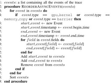
1) Building a fully coherent trace: As seen before, most of the computational intensive nodes are offloaded to the GPU, if available. The desired information about the GPU is the beginning and end times of the GPU kernels execution and memory copies. Unfortunately, it can only be collected asynchronously, once the GPU kernel or the memory copy is finished. Therefore, in the instrumentation, we use a temporary event and store the beginning and end timestamps of the GPU operation inside it. The real timestamp of this temporary event is not meaningful regarding the execution of the dataflow model, as it represents the moment when the GPU information was collected. From it, two new events are created during the post-processing phase. One corresponds to the beginning of the operation and the second to the end. Finally, we need to sort all the events according to their timestamp, since the time of a CTF trace should always increase monotonically. The pseudocode of the reordering algorithm is shown in Algorithm 1
A second concern is to insure that all the GPU-related events are coherent with the CPU-related events. Indeed, the same clock should be used. As LTTng is using the Linux Clock Monotonic, we insure that all the events in the trace are converted to this time base. Depending on the library used to program the GPU, some synchronization work might
Algorithm 1 Asynchronous events reordering algorithm 1: events: a list containing all the events of the trace
2: procedureREORDERASYNCEVENTS(events) 3: foreventineventsdo
4: if event.type == gpu kernel or event.type ==
memory copyorevent.type ==barrierthen 5: start event←new Event
6: start event.timestamp←event.begin time 7: end event←new Event
8: end event.timestamp←event.end time 9: forf ieldinevent.fieldsdo
10: start event[f ield]←event[f ield] 11: end event[f ield]←event[f ield]
12: end for
13: Addstart eventtoevents 14: Addend eventtoevents 15: Removeeventfromevents 16: end if
17: end for 18: Sortevents 19: end procedure
be required. With OpenCL, for example, the timestamps returned by the profiling functions have no specific reference and cannot be converted into a CPU time. For this reason, we need a synchronization method to connect GPU and CPU events.
When we are profiling OpenCL on the CPU for the API calls, and on the GPU for the kernel timestamps, we can get the information described in Figure 2.
Fig. 2: OpenCL profiling: Several events happen on both devices and the corresponding timestamps can be collected and used for synchronization
We can solve the synchronization problem by using this information and applying techniques like the Convex Hull algorithm presented by Poirier (2010) [34], or the more efficient version of Jabbarifar (2013) [35].
2) Matching GPU related events with the dataflow graph: The second post-processing step aims at relating the GPU operations with the dataflow model. The computation ap-proach of a GPU is that GPU kernels are enqueued into one or several queues and then the hardware schedules and executes the kernels from the queues. Moreover, a dataflow model usually contains many nodes and each can offload work to the GPU. Therefore, it is important to match the GPU kernels with the nodes in the dataflow graph. This can be implemented as a post-processing task once all the events have been collected. One limitation of this method is the
supposition that a unique queue is used to feed work to the GPU. It can be decomposed into two parts:
1) First we match all the function calls that enqueue kernels inside the GPU queue with the nodes in the graph. By using the beginning and end timestamps of the nodes in the graph, we can determine for each function call that launches a GPU kernel, the current node being executed at this moment.
2) The second part is matching the function call that enqueues kernels into the GPU queue and the real execution of the GPU kernel. For this purpose, we assumed that only one queue was used, and therefore the order of the API calls and the order of the GPU kernel executions are the same.
Finally, by combining the two parts, we are able to match all the kernels executed on the GPU with their corresponding node in the dataflow graph. After these two post-processing steps, the trace is coherent and its analysis and visualization can start. The pseudocode for the matching algorithm is available in Algorithm 2
Algorithm 2 Nodes and GPU kernels matching algorithm 1: events: a list containing all the events of the trace
2: procedureMATCHNODESWITHGPUKERNELS(events) 3: curr gpu op←None
4: curr launch cmd←None 5: foreventineventsdo
6: ifevent.type ==gpu operation beginthen 7: curr gpu op←event.name
8: else ifevent.type ==gpu operation endthen 9: curr gpu op←None
10: else ifevent.type ==launch kernel beginthen 11: ifcurr gpu op== Nonethen
12: Error, a launch command requires a current gpu oper-ation
13: else
14: curr launch cmd.op name←curr gpu op.name
15: end if
16: else ifevent.type ==gpu kernel beginthen 17: ifcurr launch cmd== Nonethen
18: Error, a GPU kernel begin event requires a current launch command
19: else
20: event.op name←curr launch cmd.op name
21: end if
22: end if 23: end for 24: end procedure
G. Analysis and Visualization
In order to profile and trace a dataflow application, the first requirement is to collect the necessary information. After, we also need to develop appropriate and helpful visualizations to display all the events in the best possible way to help identifying performance issues. For that, we developed three main elements that will be detailed later: a Callstack view, XY charts, and statistics. As the created trace is in the CTF format, Trace Compass is the best choice for the visualization. Indeed, it is a complete interactive visualization tool aiming at performance analysis of systems. Originally, it focused on operating systems analysis but was
extended for different kinds of systems. Moreover, as an open-source software, it can be easily enhanced for all kinds of needs. The main way to develop new views is with Java views, but Kouame [36] introduced a new possibility calledXML Analysis. This allows the user to rapidly develop declaratively new trace visualization views and to underline the most important parts. In our work we decided to use this option.
1) Callstack view: The Callstack view is the main part of the visualization and provides an insight into the execution of the dataflow application. It shows the state of many elements that are grouped into categories corresponding to the different characteristics of the dataflow model. Moreover, it can display nested calls or states by showing several lines. For example, one iteration of the dataflow model corresponds to feeding one batch of data to the graph and retrieving the result from the output nodes. This is a crucial information that should appear when visualizing the trace. Here are the main elements shown in the Callstack view :
• The execution of each node in the dataflow graph with the distinction between the nodes assigned to the CPU and the ones processed by the GPU.
• The beginning and end of all the calls to the functions of the libraries used to program the GPU (CUDA, HIP, HSA, OpenCL, ...)
• GPU related operations: kernels, asynchronous memory copies or synchronization barriers
• Information about the scheduling of all the operations in the graph.
With this information, the user is directly aware of the matching between the nodes of the computation graph and the physical units. Moreover, this view can be combined with Tensorboard that can graphically display the computation graph and help to understand the Callstack view.
Another important information concerns the execution of the operations on different devices. In the case of a CPU, we can easily identify the number of threads and the CPU cores used for the execution. This information is available in the Callstack view and the Resource view and require Linux Kernel tracing. In the case of an operation offloaded to the GPU, we provide textual information within the Callstack view about the division of the work. The dimension of the grid and the work groups for each GPU kernel are available. With a GPU, we are not able to have precise information about the GPU cores involved for the execution of a specific GPU kernel. The device manages the mapping between the kernel and the GPU cores by itself. Moreover, all the cores are usually identical and, even if some optimizations may be possible, they have very little impact on the performance compared to memory transfers or an efficient work division (grid dimension, work group dimension).
2) XY charts: Memory consumption is a key element for a data-centric model and XY charts are well adapted for that. When too much memory is required by an application, TensorFlow simply returns an error. It is therefore essential to know the memory consumption of each node of the graph.
By combining a XY chart representing the memory con-sumption with the Callstack view described before, the user can directly spot the nodes responsible. Several XY charts can be developed, depending on the analysis performed on the dataflow model.
In our case, with TensorFlow, a first one shows the memory allocations for each device. As explained before, only following the memory allocations performed by Ten-sorFlow might not be sufficient, especially for the GPU, as it usually allocates all the available memory at the application initialization time. Thus, an additional set of three views display more detailed information about theBFC allocator: one for the global allocator statistics, one for the chunks usage and one for the bins statistics.
For memory transfers, a XY chart is also more appropriate and displays the information in a better way, as compared to a Callstack view. Therefore, a specific view displaying all the asynchronous memory transfers was also developed.
Finally, when using TensorFlow in a distributed mode, a critical part is the communication between the machines. As most of the communication is for tensor exchanges, knowing the size of these tensors is important. Before being sent over the network, the tensor values are encoded and, by adding a single tracepoint in the encoding function, we collect the size of every tensor sent to another machine. A XY chart representing these sizes helps the user to directly identify the expensive tensor transfers between machines.
3) Statistics: Another possibility to show useful informa-tion about the execuinforma-tion of a dataflow model is to compute some statistics. This can help to quickly determine which operations in the graph took the longest time for their execution. It also allows a user to compare the execution time of a node over several executions of the graph. Obviously, in order to find the longest operations in the graph, we need to take into account the work that each node might have offloaded to the GPU. For that, we can benefit from the second post-processing step described earlier, whose goal is to associate each GPU kernel with the corresponding computation node in the dataflow graph. Apart from the duration of the execution of each node, another interesting information is the latency of the nodes in the dataflow model. Within the computation graph, a node can start being executed when all its inputs are ready. Thus, we can compute a metric representing the latency of each node by comparing the moment when the last input of a node has finished and the moment when the node actually started to be executed. In terms of implementation, we used Babeltrace to read the CTF trace, Python to compute the statistics and the results are exported into a CSV file.
H. Additional information
The goal of profiling a dataflow model is to understand the execution of the application but also to see the interactions between the different devices and to insure that all the hardware resources are used efficiently. For this purpose, two additional information can be useful and are detailed here.
1) Linux Kernel tracing: Even if some operations can offload work to the GPU and benefit from an acceleration, the global execution of the graph is managed by the CPU, possibly on several cores. Therefore, kernel traces can en-hance the userspace traces of the application and help to analyze the parallelism aspect of the computation. This is also helpful to understand the I/O operations performed by the application. With the proposed method, it is possible to collect kernel traces and display them jointly with all the events from the userspace level. Two major views exist to display the kernel traces.
• Control Flow View: It shows the state (running, waiting for CPU, blocked on I/O, ...) of every thread that was running during a tracing session.
• Resource View: It shows the state and the frequency of every CPU core, as well as the software and hardware interrupts.
The Linux Kernel traces complete our analysis environment with information from a low level layer and help users to identify and understand performance issues.
2) Performance counters: The second element addresses the performance of the GPU. The main purpose of getting support from a GPU is to speed up operations that involve heavy computation. Still today, tracing precisely the execu-tion of a kernel on the GPU is not possible and the only way to insure a good performance for the GPU kernels is by collecting performance counters. They represent hardware metrics that provide information about the execution of a kernel on the GPU. For example, we can collect counters representing the average number of vector or scalar ALU instructions executed per work-item, the number of wave-fronts, the total size of data written to or fetched from the GPU memory, or the percentage of fetch, write, atomic and other instructions that hit the data cache. These metrics give an insight into GPU kernels executions and can be helpful to ensure efficient hardware usage.
Usually, the profiling tools from the GPU vendors offer the possibility to get the performance counters for each GPU kernel of an application. In our case, we used and adapted the work of Margheritta [32] to collect the counters for every kernel invoked by the application. The result consists in a table with the rows representing the kernels and the columns the different metrics.
The analysis process is relatively easy for applications in-volving a few kernels. However, in our case, dataflow models usually entail a large number of GPU kernels, especially if we consider several executions of the graph. Therefore, we need a way to connect each kernel and the associated metrics to the node in the graph that invoked the kernel. We also need to have a time reference for each kernel as, during the profiling phase, GPU kernels can be executed several times. All of this was solved and implemented using Babeltrace and Python scripts.
IV. EVALUATION
After detailing the proposed profiling and tracing method, we evaluated its performance on a few concrete dataflow
applications. Our implementation prototype was designed for TensorFlow, so all the examples are TensorFlow applications. A. Triplet loss example
The first example is an application for face recognition that uses the triplet loss with TensorFlow, to learn good embedding of faces [37]. If we apply the tracing and profiling method described previously, we obtain the trace shown in Figure 3.
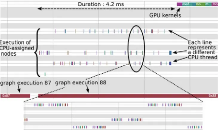
The view represents the beginning of an execution of the computational graph. As a reminder, one execution of the graph is equivalent to one call of the run() function of a TensorFlow Session and corresponds to feeding the graph with one batch of data, computing all the nodes in the graph and getting the result. For such dataflow applications, a trace usually shows the same pattern repeated several times. Each instance corresponds to one execution of the dataflow graph. Focusing on execution is a good start for the analysis.
The bottom line represents the state of the graph, if it is being executed or not. The top line corresponds to the GPU kernels executions, and all the lines in the middle represent the execution of some CPU-assigned nodes of the graph. For the sake of clarity, we hid all other information. We can see that the time between the beginning of the graph execution and the moment when the GPU actually starts to work is quite long. Even more interesting, we can notice that during this time the CPU is processing numerous nodes serially, without parallelism. Indeed, we have several threads but they are processed serially on a unique CPU core.
Fig. 3: Initial application: the beginning of the88thexecution
of the graph is shown. The GPU waits for a significant time before starting its job, and the CPU seems to inefficiently process some nodes during this time.
To continue the analysis, we can zoom in to know pre-cisely what are these nodes, as shown in Figure 4.
We can distinguish a pattern, formed out of two sequences of operations, that is repeated many times. The first sequence containsDecodeRaw,Cast,ReshapeandTruedivnodes and the second containsDecodeRaw,ReshapeandToint32 oper-ations. As they are assigned to the CPU, and are executed before the GPU started to work, we can naturally suspect that they correspond to a pre-processing step on the input
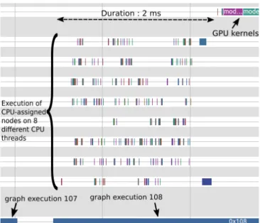
data. By looking at the source code, we can notice that these sequences of operations correspond respectively to the decode image() and decode label() functions and that both are passed as an argument to the map() function that applies them on images and labels. According to the TensorFlow documentation, the map() function offers an argument num parallel calls that allows to parallelize the processing on several CPU threads. Using this argument can reduce the time needed for this pre-processing step. Figure 5 shows the results after having set this argument to 8, the number of CPU logical cores of our machine. The resulting trace proves that the pre-processing has been parallelized on 8 threads, and the duration is now only 2 ms compared to the initial 4.2 ms.
However, we can see that the performance is still not optimal. Indeed, when the GPU starts its job (the top line), the CPU (lines in the middle) is idle. This offers the possibility to implement pipelining, so that the CPU could already pre-process the input data that will be fed into the GPU at the next execution of the graph. Indeed, nodes of the graph that are entirely executed on the CPU can naturally process data while the GPU is used by the computational intensive nodes. In this way, the data may be almost directly ready for the GPU for each execution of the graph.
TensorFlow enables this with theprefetch() function that can be applied to the dataset. Setting its argument to 1 insures that one batch of data is always ready to be fed to the GPU. Figure 6 presents the trace with the map and prefetch optimizations. It is now clear that some nodes are executed on the CPU while the GPU is processing other nodes. Obviously, the duration between the beginning of the session and the moment when the GPU starts working has significantly decreased to 790 s which corresponds to an improvement by more than5X.
As a training process with TensorFlow is made of many executions of the graph, the gain in time can be important. If we consider 500000 executions of the graph, we can quickly compute the time spent for pre-processing the data and estimate the gain:
• Original program: 500000×0.0042 = 2100 seconds ⇒35minutes
• Optimized program:500000×0.000790 = 395seconds ⇒6 minutes35seconds
It is clear that the optimized program uses the available hardware much more efficiently, which saves time.
B. Compute-bound example
As a second use case, we analyze the execution of a convolutional neural network, a very popular model when dealing with images. Figure 7 shows the trace obtained with the proposed method.
We notice here that the GPU seems to be used all the time. This behavior is desired when a CPU gets support from a GPU, since it indicates that the application fully benefits from the computing power of the GPU. In this case, we are clearly compute-bound, which reduces the improvement possibilities. However, we can still go deeper and use one of
Fig. 4: CPU-assigned pre-processing operations: The CPU processes many times these two sequences of nodes before the GPU starts.
Fig. 5: Execution with the first optimization: setting num parallel calls to 8. The processing done on the CPU has been parallelized and is more efficient now. Significant time was saved.
the proposed analysis scripts that compute statistics about the traces. One script returns statistics about the most demanding GPU kernels in terms of duration. The results, presented in Table I show the mean duration for each kernel, as well as the number of times they are executed during the whole trace. As expected, GPU kernels related to convolutions took the most time. However, theMaxpoolnodes are also noticeable in terms of duration and frequency.
Since we know that we are compute-bound, we need to reduce the amount of computation to improve the execution of the dataflow graph. We thus target the most demanding nodes. In a paper called Striving for simplicity: The All Convolutional Net, Springenberg et al [38] explained that under some conditions we can replace aConvolution + Maxpool layer by a Strided Convolution, without affecting the learning capabilities of the model. Using a strided convolution insures that the shape of the tensor after the convolution is the same as the shape of the tensor after the convolution and maxpool operations. The authors explained that no difference in final accuracy can be perceived for many image recognition benchmarks. Therefore, it is worth considering this optimization in a compute-bound situation. The Figure 8 presents the evolution of the loss and the accuracy for both cases (convolution + maxpooland
Fig. 6: Execution with the two optimizations: setting num parallel callsto 8 andprefetch to 1. In addition to the parallelization of CPU work, pipelining has been added and increases again the performance.
Fig. 7: Initial execution with the convolution and maxpool operations. The GPU seems to be in use all the time.
strided convolution) when using a basic convolu-tional neural network to classify the MNIST digits. As we can see, the learning capabilities of the model are almost not affected.
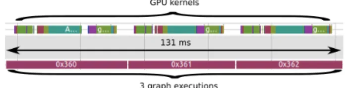
Figure 9 shows the trace at the exact same moment if we replace the convolution and maxpool nodes with a single strided convolution node. Previously, three executions of the graph took 269 ms, compared to 131 ms now, which represents a 2X benefit. As for the first example, we can do a quick estimation of the gain in terms of duration. If we consider 10000 executions of the graph, we get the following:
• Original Convolution and Maxpool:10000×0.269÷3 = 897seconds ⇒15minutes
• Strided convolution :10000×0.131÷3 = 437seconds ⇒7 minutes 12 seconds
In spite of a very small accuracy reduction, the time benefit is significant and this optimization can be suitable in many cases. This example concerns a training phase executed on a computer, but we can imagine an inference phase on a mobile device with lower computation resources, where a compute-bound situation is likely. In such a case, the model is expected to make predictions with a very low latency,
TABLE I: Most demanding nodes of the graph. Several of them are related to the MaxPool operations.
Rank Kernels Mean duration (ns) Occur. Std. dev. (ns) 1 ApplyAdam 1440119 42 238911 2 ReluGrad 1281214 14 2833 3 MaxPoolGrad 986000 14 4520 4 BiasAdd 982400 15 208916 5 MatMul 916267 15 8218 6 Relu 860133 15 3403 7 Conv2D 1 849733 45 1189160 8 MatMul 1 747714 14 7639 9 MaxPool 1 grad 586357 14 29274 10 Conv2D 1 BackpropFilter 574943 70 1140131 11 MaxPool 547533 15 45908 12 BiasAddGrad 521643 14 22292 13 Conv2DBackpropFilter 518786 28 514392 14 BiasAdd 1 446467 15 1928 15 Relu 1 429800 15 3390 16 BiasAdd 1 grad 272500 14 14912 17 MaxPool1 272500 14 14913 ... ... ... ... 62 mul 1 2000 0 14
Fig. 8: Evolution of the accuracy and the loss after 1000 iterations. The accuracy loss caused by the use of strided convolutions with no maxpool layer is subtle.
and considering this kind of optimization may help. The activation functions of the network may present a similar case. Some of them are more demanding in terms of com-putation, like ”tanh”. With the proposed method, we can easily understand the limiting elements and then possibly consider alternatives like”ReLu”, if we are compute-bound. C. Distributed Dataflow graph
With this work, we also support dataflow models dis-tributed on several machines. It corresponds to the disdis-tributed learning option in TensorFlow. In this example, we used a convolutional neural network that is distributed on two machines. This technique is named in-model parallelism. The second possibility, namedbetween-model parallelism, is not explored here but consists in replicating the same graph on several machines to learn in parallel. Finding the best partition of the graph for the device assignment is a difficult problem and there is currently no automatic way for that. Mayer R, Mayer C and Laich [39] addressed this difficult
Fig. 9: Execution with the strided convolution. The GPU is still used all the time, but the duration of 3 executions of the graph has been reduced.
problem by proposing and evaluating different strategies. Mirhoseini et al. [40] proposed an algorithm, based on machine learning techniques, to assign each node of the graph to a specific device.
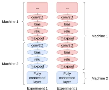
In our case, the model contains 2 convolutional layers and 1 fully connected layer. We first decided to divide the graph as follows:
• The first convolutional layer is assigned to the first machine.
• The second convolutional layer and the fully connected layer are assigned to the second machine.
For this example, we focus on the forward pass and the effects of the machine boundary between the first and second convolutional layers.
As explained in section III, the tracing and profiling happen on both machines, and the post-processed traces are gathered in one machine for the analysis and visualization step. Linux Kernel traces are collected at the same time and are necessary in order to synchronize the traces. The result is shown in Figure 10.
The view on top corresponds to the Callstack view of an execution of the graph. We can see the GPU kernels executed on the first machine, which correspond to the first convolutional layer (2D convolution and maxpool nodes). In the view, the execution of the kernels on the GPU always involves two lines, unless we are using TensorFlow with CUDA (like in the two previous examples). The purpose of the top line is to show the real names of the kernels and the line below presents the nodes of the graph responsible for the execution of the GPU kernel. The long line in the middle represents a wait time for the second machine. It starts when the second machine sends the request to the first computer for the result of the first maxpool layer, and ends when the result has arrived on the second computer and can be used as the input for the second convolutional layer.
The XY chart under the Callstack corresponds to the tensor encoding. Before being sent over the network, tensor values are encoded and the line represents the time spent for this, as well as the amount of data that is sent. The encircled operations on the right, prove that the second machine actually received the data. They correspond to asynchronous memory copies from the host (CPU RAM) to the device (GPU memory) on the second machine. The amount of data sent by the first machine corresponds to the amount of data copied into GPU memory on the second machine: 51380224 bytes. Moreover, we can compute the same result with the
Fig. 10: Distributed execution of a CNN on 2 machines - first experiment. Machine 1 executes the first convolutional layer and the machine 2 asks for the result. Once received, machine 2 can compute the second convolutional layer and the dense layer. The XY chart at the bottom shows the size of the tensors exchanged between the machines.
shape of the tensor after the first maxpool operation and the batch size:2048×14×14×32×4 = 51380224. Around 600 ms is spent to transfer the result between the machines. As the time required to send the tensor represents a large percentage of the execution time (around 2 s), we decided to change the partition of the graph.
In a second experiment, both convolutional layers are assigned to the first machine, and the fully connected layer to the second machine, as shown in Figure 11.
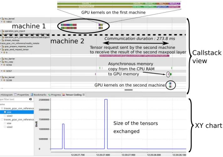
Again the application is traced and profiled and the result is compared with the first experiment, shown in Figure 12. We can recognize a similar pattern as before, but also note that the time spent for the communication has been reduced to 273.8 ms. Obviously, this is related to the size of the data exchanged between the machines. Applying a second maxpool operation decreases the size of the tensor, which results in a total size of: 2048×7×7×4 = 25690112 bytes.
Knowing that, we can conclude that the second way of splitting the graph may be more suitable, as the duration of the communication decreased. Since the dataflow model is supposed to be executed many times, the gain can be very important regarding the complete training process. Moreover, here the focus is on a single data transfer between the ma-chines and only for the forward pass. In a real optimization
Fig. 11: Division of the graph for both experiments.
process, we should have considered all the data transfers between the machines and also for the backward pass.
Through this example, we showed that the view obtained with the proposed tool is helpful and brings valuable in-formation to the user. The user can see a detailed trace of
Fig. 12: Distributed execution of a CNN on 2 machines - second experiment. This time, machine 1 executes the two convolutional layers and machine 2 asks for the result. Once received, machine 2 can compute the dense layer. The XY chart at the bottom shows that the size of the tensors exchanged between the machines is reduced compared to the first experiment.
the execution: where each operation is executed, how much data is transferred, the transfer direction, the time spent in communication, etc.
In our case, the two machines were similar, but this information can be even more valuable if the two or more machines have different characteristics (GPU vs no GPU) and capabilities (number and frequency of the CPU and GPU cores, memory, ...). For this simple example, only two machines were used but the proposed tool can handle large distributed clusters of machines.
D. Inference example
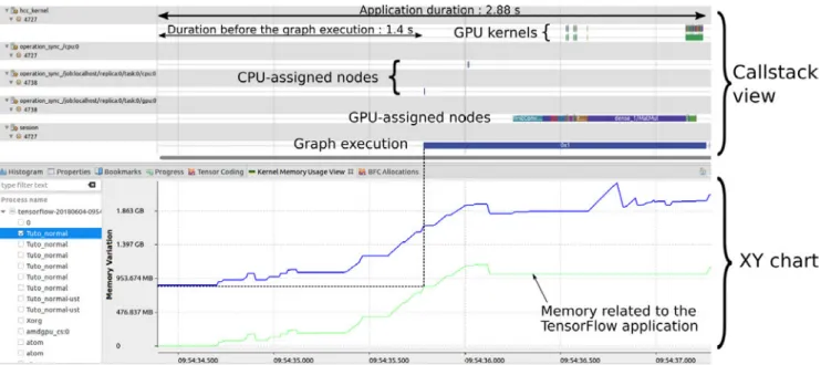
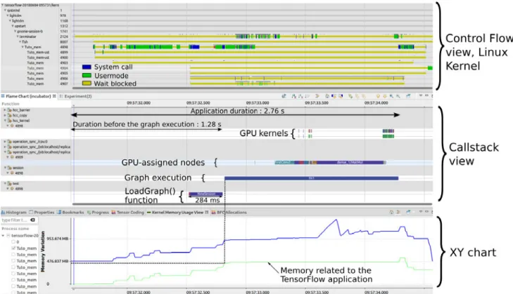
Dataflow graphs are usually intended to be executed many times, but there are a few exceptions. For example, an inference step with machine learning model may consist of a single execution of the graph. On mobile devices, for example, we can have a trained model to classify flowers and want to know the name of a flower in one new image. Figure 13 shows the Callstack view obtained if we trace and profile the application.
The first thing we notice is that the time spent by the execution of the dataflow graph only represents a fraction of the total execution time. 1.4 s is spent before the execution
of the graph. With the Kernel Memory Usage view of Trace Compass, we can also see the amount of RAM memory used by the application. This is represented by the bottom line in the XY chart and is around 800 MB at the beginning of the graph execution. In the Callstack view, we do not have real information about what is happening before the beginning of the execution of the graph. This is therefore a good example where the Linux Kernel tracing is useful. With this information, we see that a thread was processing and made several system calls (in blue). If we zoom in, we note that many of these arepread calls, which suggests that the application spends a lot of time reading a file.
We know that the application has to load the trained model and the learned weights before being able to make predictions. Looking at the source code, we can find a LoadGraph() function. As the profiling environment is very flexible, it is easy to quickly instrument this function and to display the result in the Callstack view, together with all the other elements. The instrumentation of LoadGraph() is separated in two:
• Reading binary: the first small rectangle (red) in figure 15
Fig. 13: Initial Callstack and Linux Kernel memory usage views for an inference step. A long time is spent before the beginning of the graph execution and around 800 MB of RAM memory is used by the TensorFlow application.
Fig. 14: Kernel traces of the inference step. We can detect a lot ofpread system calls. They correspond to the loading of the model file.
figure 15
We can also measure that the LoadGraph() function call lasted around 400 ms. Figure 15 shows the result and proves that this function indeed took some time.
TensorFlow proposes a complete and well-documented performance guide that introduces a way to load model files more efficiently. This method is a memory mapping technique that maps directly the file into RAM memory. This prevents allocating memory on the heap and then copying bytes from the file into this allocated space. When using this method, we get the result shown in Figure 16 and we can note a few elements:
• The total time spent before the beginning of the graph execution has been reduced to 1.28 s (1.4 s previously)
• The duration of the LoadGraph() function (reading binary + creating a new session) has decreased to 284 ms (400 ms previously).
• The kernel memory usage of the dataflow application is now around 450 MB, as compared to 800 MB
previously.
• As the duration of the graph execution did not change, the total duration of the application gets the same reduction as the loading step: 2.76 s (2.88 s previously) Through this example, another advantage of our method is pointed out. In addition to a precise profiling of the dataflow graph, we can also benefit from other useful information like the Linux Kernel traces as well as the possibility to easily integrate an external instrumentation of the application. E. Memory management example
The last example is about specific situations where the memory management of the dataflow model is problematic. When the majority of the nodes are GPU-accelerated and the dataset can fit into the GPU memory, one large memory copy is probably more efficient than several smaller copies. With TensorFlow, we can imagine an example where the computation graph simply consists of asquareoperation on a matrix (square of the matrix element-wise) and areduce sum operation that sums all the elements of the matrix. The
Fig. 15: Callstack and kernel status, with the static instrumentation of the LoadGraph function. We can verify that this function is indeed time consuming.
Fig. 16: Kernel traces, Callstack and Linux Kernel memory usage view of the optimized application. Using the memory mapping technique to load the model file decreases the duration of theLoadGraph function. The RAM memory usage is also decreased at the beginning of the graph execution, compared to the first version of the application.
classic technique consists in feeding a batch of data to the computational graph in TensorFlow at the beginning of each graph execution. Moreover, as the computation nodes of the graph are assigned to the GPU, the data is also copied from the CPU to the GPU. Figure 17 shows the profiling and tracing of one execution of the graph.
Fig. 17: Normal execution using feed dict argument. An important percentage of the execution is dedicated to a large memory transfer from the RAM memory to the GPU memory.
We clearly notice that there is a long memory copy from the Host (CPU) to the Device (GPU), and that it took much more time than the computation part that follows. Thesquare andsum operations are indeed relatively quickly computed on the GPU and this emphasizes the long time spent in the memory copy. At each execution, a new batch of data is created from the dataset and given to the graph as input. Thus, this phenomenon repeats at each execution of the graph, which means that a very large percentage of the total application time is related to memory copies from the CPU to the GPU.
If the dataset is not too large and can fit into the GPU memory, another option may be more efficient. It consists in copying the whole dataset once to the GPU memory and then adding a new node into the dataflow graph that creates the batches from the whole dataset. In spite of requiring additional time to perform the copy of the dataset once, all the executions of the graph afterward are much faster, as shown in Figure 18.
Almost all the execution time is now dedicated to the computation part performed by the GPU, and the total time