Proceedings of 7th Transport Research Arena TRA 2018, April 16-19, 2018, Vienna, Austria
A probabilistic framework for traffic data quality
Rüdiger Ebendt*, Thorsten Neumann
Institute of Transportation Systems, German Aerospace Center (DLR), Rutherfordstr. 2, 12489 Berlin, Germany
Abstract
Regarding the assessment of traffic data quality in ITS, there is an increasing demand for answers to the following questions: (i) what exactly is "traffic data quality"? and (ii) how can the incomparableness and inconsistency of results from different researchers be avoided? To this end, an important aim of the ongoing project I.MoVe of German Aerospace Center (DLR) is to develop a consistent understanding of traffic data quality, together with a unified framework for its assessment. In this paper, the resulting probabilistic framework based on established criteria like accuracy, validity, coverage etc. is provided. Real-world examples demonstrate its application for the assessment of data sources like induction loop detectors, stationary Bluetooth sensors and floating car data (FCD). The provided examples include the assessment of loop count accuracy, and of the temporal coverage of a) a measurement track with stationary Bluetooth data, and of b) FCD for Berlin, Germany. Keywords: Quality; data quality; probability; traffic data.
* Corresponding author. Tel.: +49-30-67055-287 ; fax: +49-30-67055-291 . E-mail address: [email protected]
1.Introduction
There is an increasing demand for answers to the following questions regarding the assessment of traffic data quality in ITS: i) what exactly is "traffic data quality"? and, related to that, ii) how can the incomparableness and inconsistency of results from different researchers be avoided? To this end, an important aim of the ongoing project I.MoVe from German Aerospace Center (DLR) is to develop a consistent understanding of traffic data quality, together with a unified framework for its assessment. In this paper, the resulting probabilistic framework is provided. A first important point is to distinguish strictly between quality indices, quality requirements, and quality itself. While the present framework develops quality indices based on established quality criteria like accuracy, completeness, validity, and coverage (see Turner (2004), Federal Highway Administration (2004)), the usual understanding of quality as defined in Crosby (1979) or International Organization for Standardization (1992) is extended to a probabilistic view. This also addresses the problem of information retrieval in the presence of vagueness and uncertainty: typically, a census, i.e. a complete enumeration of quality measures determined for all vehicles in the population is impractical or impossible. Therefore, measures for traffic data quality are usually estimated from empirical data. Random samples are collected and statistics are calculated from them, allowing for inferences from the sample to the population.
Real-world examples from I.MoVe demonstrate the application of the proposed framework for the assessment of data sources like induction loop detectors, stationary Bluetooth sensors and floating car data (FCD). They include the assessment of induction loop count accuracy as well as assessing the temporal coverage of a stretch of road with stationary Bluetooth data, and of the whole city of Berlin, Germany with FCD. The provided examples also constitute interesting results for the practitioner.
The paper is structured as follows. In Section 2, the new probabilistic view on quality is motivated. A formal framework for this view is given in Section 3. Section 4 summarizes the advantages of the proposed framework, and Section 5 gives practical examples from the DLR project I.MoVe, demonstrating its advantages. Finally, the work is concluded in Section 6.
2.A probabilistic view on quality
The two most notable definitions of quality are from Philip B. Crosby and the International Organization for Standardization (ISO). According to Crosby (1979), quality is “conformance to requirements”. There are similar definitions in published standards like the IEC 2371 and the German DIN 55350, part 11. In International Organization for Standardization (1992), quality is defined as “degree to which a set of inherent characteristics fulfills requirements”, a definition still used in the current ISO norm 9000:2015-11. In Turner (2004), and Federal Highway Administration (2004), a set of measures for traffic data quality has been proposed: accuracy, completeness, validity, timeliness, coverage, and accessibility. Four of these six measures are defined as a degree of fulfilment of requirements: e.g. completeness is defined as the (percentage) degree to which data values are present in attributes that require them (such as e.g. traffic volume and speed). At first glance, the view on traffic data quality as a degree of fulfilment of (application-dependent) requirements as used here may seem more detailed than the very compact definition of Crosby (1979) as “conformance to requirements”. The latter definition focuses on a Boolean representation of quality (as the possible answers “yes” or “no” to the question “conformant to requirements?”), while the previous definition allows for expressing a degree of fulfilment of the requirements as a continuous, ratio-scaled percentage. But e.g. for the degree of fulfilment of completeness, what exactly is expressed if one states that e.g. the present data has complete and valid data attributes up to a degree of 94%? This implicitly states a degree of fulfilment with regard to the underlying requirement of full completeness (i.e., one requires the data to be totally valid and complete attributes). But then any degree below 100% would mean that the actual requirement has not been fulfilled. This could already be expressed by the simple answer “no”, and therefore the extra information of the exact degree of fulfilment would not change the formal decision on the fulfilment of the requirement. Moreover, for a practitioner, requiring 100% of the data to be valid and complete may seem overly restrictive.
Thus, another and better way of interpretation of the percentage is to see this information as the observed quality measure only, and not as the quality itself. That way, the actual assessment of quality (i.e., “Is 94% completeness good or bad?”) has been left open, whether it be because the need for it is simply disregarded (which is bad), or because the momentary lack of a settled quality requirement for the considered application forces a
postponement. Such an application-dependent requirement usually has the form of a stated threshold for acceptance, e.g. a minimum percentage of 95% completeness in the travel time data used for the operation of an ATIS (stated as “quality target” in Federal Highway Administration (2004)), or, alternatively, of several stated thresholds defining various levels of quality in the sense of a graded fitness for a particular purpose. E.g., ITS America and U.S. Department of Transportation (2000) defined a richer range of quality levels like “good”, “better”, and “best”, and provided specific quality level criteria for each attribute. For example, five to ten percent error in travel times and speeds was classified as a “better” quality level of accuracy. But then assessing the quality again means answering questions like “is the observed measure greater than or equal to the numerical threshold?” with an answer “yes” or “no”. Notice that also the seemingly simpler definition of quality in Crosby (1979) already works with the terms “requirements” (in the sense of e.g. a threshold), and “conformance” (implying a comparison of quality indicators or measures to requirements). Consequently, while the linguistic presentation of Crosby’s definition is conveniently compact and precise, it is just as detailed or general as the definition in e.g. Turner (2004), i.e. as the degree of fulfilment of requirements which just insinuates that there are more than two possible quality levels considered.
In contrast to that, this section aims at a real generalization of the definition in Crosby (1979). The motivation is as follows: measures for traffic data quality are usually estimated from measured empirical data. Typically, a census or a complete enumeration of quality measures determined for all vehicles in the population is impractical or impossible because of the sheer size of the underlying population of vehicles. Instead, random samples are collected and statistics are calculated from them, allowing for inferences from the sample to the population. The required inferences are mathematical statistics, and they are made under the framework of probability theory, which considers the probability distributions underlying the traffic data. The usual approach is to draw a random sample 𝑆𝑆 from the population Ω, and quality measures are calculated for its |𝑆𝑆| elements. The probability that the quality measure 𝑥𝑥 determined for a new object from Ω fulfils the quality requirements is assumed to be
𝑃𝑃(𝑥𝑥 fulfils requirement(s)) = |𝐸𝐸| |𝑆𝑆|⁄ , where 𝐸𝐸 ⊆ 𝑆𝑆 is the subset of elements in 𝑆𝑆 whose quality measures fulfil the requirement(s). For example, consider again the quality measure for completeness as suggested in Federal Highway Administration (2004): it is the percentage to which data values are present in the attributes that require them, or more precisely, 𝑞𝑞completeness=𝑛𝑛available_values
𝑛𝑛total_expected ∙ 100%. Let us assume that this percentage is 90%. With the
previous terminology and notation, we have that |𝐸𝐸| = 𝑛𝑛available_values and |𝑆𝑆| = 𝑛𝑛total_expected, and that
𝑃𝑃(𝑥𝑥 indicates presence of required values) = 𝑃𝑃(𝑥𝑥 fulfils completeness requirement(s)) = |𝐸𝐸| |𝑆𝑆|⁄ = 0.9. The quality measure 𝑞𝑞completeness is a degree of fulfilment of an implicitly presumed requirement of total (i.e., 100%) completeness in the data values. This opposes to 𝑃𝑃(𝑥𝑥 indicates presence of required values), which expresses the probability that the quality measure 𝑥𝑥 of a new, unspecified object from Ω indicates the presence of all required values for the object attributes. This probability has been estimated, and the estimation has been based on a sample, drawn randomly from a population of unmanageable size. The outlined shift to a probabilistic view motivates an extended, more general definition of the term “quality”. In the previous paragraphs, it had already been outlined that quality is “conformance to requirements”, implying that it is tested whether quality measures fulfil an application-dependent quality requirement. As has been outlined, this test has a statistical or probabilistic nature, and it seems appropriate to account for this in the definition of quality. Therefore, the authors propose the following definition of quality:
“Quality is the probability of conformance to requirements”
Notice that the Boolean qualities of Crosby (1979) are a special case of this definition. They are involved if quality is measured directly for a particular object of interest. Then, the quality requirement can be tested directly with the quality measure obtained for this particular object (thereby assuming that the measurement error is negligible). Consequently, there are only two possible outcomes of the test, namely “requirement is fulfilled” or “requirement is not fulfilled”. Hence, it must be 𝑃𝑃(𝑥𝑥 fulfils the requirement(s)) = 1 if the outcome is “requirement is fulfilled” and it must be 𝑃𝑃(𝑥𝑥 fulfils the requirement(s)) = 0 if the outcome is “requirement is not fulfilled”. Thus, Crosby’s Boolean qualities can be rediscovered, modelled as degenerate (or Dirac) probability distributions. Consequently, the above proposal for a probabilistic definition of quality is a real generalization of Crosby´s definition. The next section lays the ground for the new definition of quality by giving a formal framework. After that, its benefits are described in Section 4, and its use demonstrated by real-world examples from the assessment of traffic data quality in Section 5.
3.Quality, quality requirements, quality measures: a formal framework
This section gives a formal framework for the probabilistic definition of quality. A first aim is to separate the terms quality, quality requirement, and quality measures cleanly. Quality is defined as the probability of conformance to requirements (see Section 2). In practice, so-called quality measures are calculated from the measured attributes of the objects of interest, and these measures are inspected to examine whether a quality requirement (or a whole set of quality requirements) is (are) fulfilled. Quality measures are numerical descriptors usually calculated from measurements, which are assignments of a numerical value to an observed attribute. If measurement of the attributes is not possible, one may still resort to using empirical values from previous studies, from the manufacturer’s data for quality (e.g., for accuracy or service life), or from mere rules of thumb. Quality, i.e. the probability of fulfilment of certain requirements can be defined then:
a) for the quality measure of a particular single object of interest (i.e. for a sample of size 1) b) for an unspecified element from the whole population based on a sample with multiple elements c) for the aggregated quality measure of a set of objects drawn from the population
Case a) relates to direct measurements or estimates of the quality for only one particular object of interest, whereas cases b) and c) aim at estimations based on several objects drawn from the population. In case c), the quality measure can be similar to e.g. the mode, to a moment or central moment for continuous data types. A practical example would be an error rate measuring accuracy like e.g. the MAPE. For categorical data, typically frequencies and percentages are used. Notice that the sample is a singleton in case a) as well as in case c). Let 𝑋𝑋 be the set of all possible outcomes of quality measure calculation from measured object attributes (typically,
𝑋𝑋 ⊆ ℝ). Formally, a quality requirement is a Boolean function 𝑓𝑓: 𝑋𝑋 → {0,1} such that
𝑓𝑓(𝑥𝑥) = �1 if requirement for 𝑥𝑥 is fulfilled0 otherwise
A quality requirement induces a particular event, namely the set 𝐸𝐸 ⊆ 𝑋𝑋 of quality measures which fulfil the quality requirement, i.e. 𝐸𝐸 = {𝑥𝑥|𝑥𝑥 fulfils the requirement}. This can be used to simplify the notation of 𝑓𝑓 to
𝑓𝑓 = 1𝐸𝐸 where 1𝐸𝐸: 𝑋𝑋 → {0,1} is the indicator function for 𝐸𝐸 ⊆ 𝑋𝑋. For a quality requirement 𝑓𝑓 and arbitrary additional information 𝐼𝐼, ℚ = ℙ(𝑓𝑓(𝑥𝑥) = 1) is called an a priori quality, and ℚ = ℙ(𝑓𝑓(𝑥𝑥) = 1|𝐼𝐼) is called a conditional quality. The latter, in particular, takes into account that the result of a quality assessment may change if further knowledge about the object under consideration becomes available. The estimated (probabilistic) quality of a given traffic data set, for instance, naturally depends on how much is known about the true traffic states as measured by additional sensors or not. Moreover, the dependence on 𝐼𝐼 definitely holds in case of quality assessment for modelled or simulated traffic conditions when these are augmented by real-world measurements as a realistic scenario in traffic monitoring.
Case a) as described at the beginning of this section corresponds to the case where (under neglect of measurement errors) the information 𝐼𝐼 about fulfilment or non-fulfilment of the quality requirements can in certain situations be obtained directly as this requires inspection of one object only. If so, the resulting (i.e, conditional) quality is either
ℚ = ℙ(𝑓𝑓(𝑥𝑥) = 1|𝑓𝑓(𝑥𝑥) = 1) = 1 (1a)
or
ℚ = ℙ(𝑓𝑓(𝑥𝑥) = 1|𝑓𝑓(𝑥𝑥) = 0) = 0 (1b)
That is, the conditional probabilities in Eqs. (1a) and (1b) comply with a degenerate (or Dirac) probability distribution (which can be thought of modelling a two-headed coin). Needless to say, this corresponds to the Boolean definition of quality by Crosby (1979). Clearly, the Eqs. (1a) and (1b) in principle also hold in cases b) and c) from above. However, from a practical point of view, it is much more difficult (or even impossible) to obtain such exact information 𝐼𝐼 for the considered conditionals because of the missing specification of the analyzed element as in case b) and/or the (potentially) large number of elements that have to be analyzed as in case c). Thus, there is even more need for a generalized (i.e. probabilistic) view on quality in cases b) and c).
Note that, of course, the probabilistic approach is helpful in case a) as well when measurements as described above are not possible or when measurement errors are too large as to be neglected.
In practice, a quality requirement 𝑓𝑓 often makes use of a threshold, i.e. 𝑓𝑓 returns 1 for an argument 𝑥𝑥 i) not exceeding, or alternatively, ii) not falling below a given threshold 𝑐𝑐thresh, and otherwise returns 0. Then 𝑓𝑓 is an
indicator function for which we have 𝑓𝑓 = 1𝐸𝐸 where 𝐸𝐸 = {𝑥𝑥 ≤ 𝑐𝑐thresh} in case i) and 𝐸𝐸 = {𝑥𝑥 ≥ 𝑐𝑐thresh} in case ii).
Moreover, in case i) it is ℚ = ℙ(𝑓𝑓(𝑥𝑥) = 1) = ℙ(𝑥𝑥 ≤ 𝑐𝑐thresh), and in case ii) we have ℚ = ℙ(𝑓𝑓(𝑥𝑥) = 1) =
ℙ(𝑥𝑥 ≥ 𝑐𝑐thresh). Further, let 𝐹𝐹𝑥𝑥 denote the cumulative distribution function (CDF) of a random variable 𝑥𝑥, taking on outcomes in 𝑋𝑋 as its realizations. Then we have that ℙ(𝑥𝑥 ≤ 𝑐𝑐thresh) = 𝐹𝐹𝑥𝑥(𝑐𝑐thresh) and that ℙ(𝑥𝑥 ≥ 𝑐𝑐thresh) =
1 − 𝐹𝐹𝑥𝑥(𝑐𝑐thresh) + ℙ(𝑥𝑥 = 𝑐𝑐thresh).
If more than one quality requirement is used, the semantics usually comply with one of the following cases: 1) The quality measures are required to fulfil all quality requirements.
2) Every quality measure fulfils exactly one of the quality requirements.
Case 1) can be reduced to the case of using only one quality requirement: to this end, the pointwise product of all quality requirements is chosen as the quality requirement: let (𝑓𝑓𝑖𝑖)𝑖𝑖=1,…,𝑛𝑛 be a family of quality requirements respecting the condition of case 1). Then, for the observed quality measures 𝑥𝑥, we have (𝑓𝑓1∙ 𝑓𝑓2∙ … ∙ 𝑓𝑓𝑛𝑛)(𝑥𝑥) =
1 ⇔ 𝑓𝑓1(𝑥𝑥) ∙ 𝑓𝑓2(𝑥𝑥) ∙ … ∙ 𝑓𝑓𝑛𝑛(𝑥𝑥) = 1 ⇔ 𝑓𝑓1(𝑥𝑥) = 1 and 𝑓𝑓2(𝑥𝑥) = 1 and ⋯ and 𝑓𝑓𝑛𝑛(𝑥𝑥) = 1, and (𝑓𝑓1∙ 𝑓𝑓2∙ … ∙ 𝑓𝑓𝑛𝑛)(𝑥𝑥) =
0 ⇔ 𝑓𝑓1(𝑥𝑥) ∙ 𝑓𝑓2(𝑥𝑥) ∙ … ∙ 𝑓𝑓𝑛𝑛(𝑥𝑥) = 0 ⇔ 𝑓𝑓1(𝑥𝑥) = 0 or 𝑓𝑓2(𝑥𝑥) = 0 or ⋯ or 𝑓𝑓𝑛𝑛(𝑥𝑥) = 0. Case 2) follows the idea of partitioning 𝑋𝑋 into events, each of which corresponds to one of several disjoint quality levels. The partition is constituted by a family of pairwise disjoint events, the union of which equals 𝑋𝑋. By that, every object of interest is assigned to exactly one of the quality levels. More precisely: let (𝑓𝑓𝑖𝑖)𝑖𝑖=1,…,𝑛𝑛 be a family of quality requirements respecting the condition of case 2). Let 𝑥𝑥 ∈ 𝑋𝑋. Since 𝑥𝑥 fulfils exactly one of the quality requirements, 𝑥𝑥 must be contained in exactly one of the sets 𝐸𝐸𝑖𝑖∶= {𝑥𝑥|𝑓𝑓𝑖𝑖(𝑥𝑥) = 1}, 𝑖𝑖 = 1, … , 𝑛𝑛. Therefore we have
� 𝐸𝐸𝑖𝑖= 𝑋𝑋and𝐸𝐸𝑖𝑖∩ 𝐸𝐸𝑗𝑗 = ∅
𝑖𝑖 for all𝑖𝑖 ≠ 𝑗𝑗 (2)
That is, the sets (𝐸𝐸𝑖𝑖)𝑖𝑖=1,…,𝑛𝑛 (corresponding to events) are a partition of 𝑋𝑋. For ℚ𝑖𝑖∶= ℙ(𝐸𝐸𝑖𝑖) we have
∑ ℚ𝑖𝑖 𝑖𝑖=∑ ℙ(𝐸𝐸𝑖𝑖 𝑖𝑖) = ℙ(⋃ 𝐸𝐸𝑖𝑖 𝑖𝑖) = ℙ(𝑋𝑋) = 1 by (2). Often, the quality requirements corresponding to different levels of quality are expressed with thresholds, e.g. 𝐸𝐸1= {𝑥𝑥|𝑥𝑥 ≤ 𝑐𝑐thresh1} corresponding to a first quality level,
𝐸𝐸2= {𝑥𝑥|𝑐𝑐thresh1< 𝑥𝑥 ≤ 𝑐𝑐thresh2} corresponding to a second, and so on, where 𝑐𝑐thresh1< 𝑐𝑐thresh2< ⋯. Again, CDFs can be useful for convenient calculation of the corresponding probabilistic qualities, e.g. the probability of an unspecified sample element to be contained in 𝐸𝐸2 is ℙ(𝑐𝑐thresh1< 𝑥𝑥 ≤ 𝑐𝑐thresh2) = 𝐹𝐹𝑥𝑥(𝑐𝑐thresh2) − 𝐹𝐹𝑥𝑥(𝑐𝑐thresh1). Finally, when comparing two or more objects based on their probabilistic qualities ℚ(𝑘𝑘)= ℙ(𝑓𝑓(𝑥𝑥) = 1),
𝑘𝑘 = 1, … , 𝑚𝑚, with regard to the same requirement function 𝑓𝑓, it is clear that object 𝑘𝑘 is better than object 𝑙𝑙 in terms of 𝑓𝑓 iff ℚ(𝑘𝑘) > ℚ(𝑙𝑙) and vice versa (an example can be found at the end of Section 5.2.2). Moreover, in case of a partitioned 𝑋𝑋 as above with ordered quality levels 𝐸𝐸𝑖𝑖 (from lowest to highest), the concept of first order stochastic dominance (SD), known from the context of risky financial options (cf. Levy (1992)), can be applied to the corresponding ℚ𝑖𝑖(𝑘𝑘) as related to the 𝑘𝑘-th object. That is, let 𝑆𝑆𝑖𝑖(𝑘𝑘)≔ ∑𝑖𝑖𝑗𝑗=1ℚ𝑗𝑗(𝑘𝑘) be the cumulative probabilistic qualities for object 𝑘𝑘, representing the CDF of the discrete probability distribution given by
�ℚ𝑖𝑖(𝑘𝑘)�𝑖𝑖=1,…,𝑛𝑛. Then, object 𝑘𝑘 performs better than object 𝑙𝑙 if 𝑆𝑆𝑖𝑖(𝑘𝑘)≤ 𝑆𝑆𝑖𝑖(𝑙𝑙) for all 𝑖𝑖 and 𝑆𝑆𝑖𝑖
𝑜𝑜
(𝑘𝑘)< 𝑆𝑆 𝑖𝑖0
(𝑙𝑙) for at least one
𝑖𝑖0. Note that it is possible in this context that two given objects are not comparable as SD generates an only partial order on the set of all objects (for an example, see Fig. 1b).
4.Benefits of the probabilistic framework
Quality as proposed by Crosby basically is a Boolean quantity, modelled by e.g. a dichotomous random variable representing the possible answers “yes” or “no” (i.e., requirements are fulfilled or not). Quality as proposed by the authors is a probability. An advantage is that probabilities provide much more detailed information, and that – in contrast to the usage of the vague term “degree” in the applicable ISO norms – the proposed framework explicitly complies with probability theory. Thereby, it provides a well-known formal calculus and also a wider range of possible subsequent calculations with qualities. For instance, consider the situation that an assessment of quality occurs repeatedly, and very often. Then, the spatially and/or temporally distributed outcomes of
quality assessment can be modelled by a discrete or continuous random variable, and by the respective probability distribution (for an example of a spatial distribution of qualities see Section 5.1.1., for an example of a temporal distribution of qualities see Section 5.1.2). Ratios of probabilities are meaningful since a (unique and non-arbitrary) zero value exists (a probability of zero characterizes an impossible event). Consequently, the coefficient of variation (COV) is allowed to measure the statistical dispersion of the aforementioned distribution of qualities. Moreover, the framework facilitates and sanitizes the construction of composite qualities: for that purpose, a conjunction of the quality requirements can be used as in Section 3, case 1). Another possibility is to consider the joint probability distribution of the various qualities, allowing for the calculation of marginal probabilities, e.g. of the probability that all quality requirements are fulfilled (for example of “composite system completeness”, if the quality of coverage, completeness, and validity is considered), or of composites of only a subset of the assessed qualities, such as e.g. the quality of “valid completeness” (a composite of the quality of validity and the quality of completeness) or of “coverage completeness” (a composite of the quality of coverage and of the quality of completeness). Notice that this is a generalization of the proposal to use composite quality measures in Federal Highway Administration (2004). Moreover, also conditional probabilities or entropy measures as used in information theory (cf. Klir (1991)) can be calculated as subsets of the joint probability distribution, if they are of interest in the context of the considered application.
In contrast to previous proposals for composite qualities like in Federal Highway Administration (2004), and to the practice of many research papers, no (weighted) averages of purely ordinal “scores” assigned to different numerical ranges of quality measures need to be calculated here. Notice that it has been controversial whether calculating measures of central tendencies like the mean or the standard deviation from purely ordinal data (like e.g. grade-point averages or the equivalent in many educational systems) is valid in all cases (see e.g. Knapp (1990)), and that there are cases where this practice is commonly considered as illegitimate, see e.g. Sullivan and Artino (2013).
5.Practical examples
During the last decade, German Aerospace Center (DLR) has established several web-based traffic monitoring systems, e.g. KeepMoving (see Brockfeld (2014)). Data sources for these systems include floating car data (FCD), data from stationary Bluetooth detectors and from induction loop detectors. During the DLR project I.MoVe, the quality of data from all these sources has been assessed. The following examples from I.MoVe demonstrate probabilistic qualities for an unspecified object of a given population based on a (sufficiently large) sample, corresponding to case b) in Section 3. Besides case c), this is the case occurring most frequently in the assessment of traffic data quality, since in practice direct measurements during a census are rarely workable. 5.1. Assessment of the quality of temporal coverage
5.1.1. Floating car data (FCD)
DLR continuously collects FCD in Berlin, Germany. The raw FCD are vehicle trajectories from more than 6,000 taxis, equipped with on-board GPS receivers. The trajectories are sequences of time-stamped GPS positions. During an online data-procession including a map matching procedure, mean link travel speeds are computed for every five minutes and for every link of a digital road map (if no current FCD are available on an edge, a historical mean speed value is used). Quality measures of coverage are a useful complement to other measures like e.g. measures of accuracy or timeliness. Besides the spatial coverage, measures of temporal coverage are used to assess the quality measured by the number of received position reports per time interval, see e.g. Szigeti, Laborczi and Gordos (2007). In terms of the definitions proposed in Section 3, a quality measure
𝑞𝑞temporal_coverage=𝛥𝛥𝛥𝛥𝑛𝑛, i.e. the number of position reports 𝑛𝑛 received on a link per time interval 𝛥𝛥𝛥𝛥 is calculated, and the respective quality requirement is 𝑛𝑛
𝛥𝛥𝛥𝛥≥ 𝑐𝑐minimum. Reference values for the threshold 𝑐𝑐minimum are based on previous experiences in research and depend on the application (e.g. on traffic planning or traveler information), and can be found in the literature, e.g. Davidsson, et al. (2002). An alternative to this assessment with fixed reference values 𝑐𝑐minimum is given in Turner and Holdener (1995), and Srinivasan and Jovanis (1996): in order to arrive at statistically justified thresholds for a given stretch of road and a chosen observation period, one calculates the number 𝑛𝑛𝑟𝑟 of position reports required to guarantee a desired degree 𝑟𝑟 of “reliability” of the computation of mean link travel times in this period. That is, 𝑟𝑟 is defined as the desired probability (e.g. 𝑟𝑟 = 0.95), that the absolute percentage error of the mean link travel times is smaller than a desired maximal error
𝑒𝑒max of e.g. 0.1. Notice that the quality of the processed data is assessed, not the quality of the sensors / of the acquisition of raw data (which may be good even when the temporal coverage is too low to calculate reliable travel times). It can be shown that we have 𝑐𝑐minimum= 𝑛𝑛𝑟𝑟= �𝛷𝛷−1((1+𝑟𝑟)/2)
𝑒𝑒max∙𝜇𝜇𝜎𝜎 �
2
, where 𝜇𝜇 is the mean of the travel times in the respective period, 𝜎𝜎 the respective standard deviation, and Φ−1(∙) is the inverse of the CDF of the standard normal distribution (see Srinivasan and Jovanis (1996)). For the values in the above example (𝑟𝑟 = 0.95,
𝑒𝑒max= 0.1), one obtains 𝑛𝑛𝑟𝑟= �𝛷𝛷
−1((1.95/2) 0.1∙𝜇𝜇𝜎𝜎 � 2 ≈ �19.60𝜇𝜇 𝜎𝜎 � 2 = �19,60 ∙𝜎𝜎𝜇𝜇�2. By an application-dependent use of different values for 𝑟𝑟 and 𝑒𝑒max, different formulas for thresholds 𝑛𝑛𝑟𝑟 can be derived, each depending on the sample mean and standard deviation, corresponding to different quality levels for the respective application. Table 1 gives an instructive example for such a set of quality levels. Quality requirements for applications like traffic planning, traffic management, and travel information / ATIS are described in e.g. ITS America and U.S. Department of Transportation (2000), Tarnoff (2002), and Federal Highway Administration (2004).
Table 1: Example of quality levels for temporal coverage Chosen reliability (𝒓𝒓) and maximal error
(𝒆𝒆max)
Formula for threshold 𝒏𝒏𝒓𝒓 𝒓𝒓 = 𝟎𝟎. 𝟗𝟗𝟗𝟗, 𝒆𝒆max= 𝟎𝟎. 𝟏𝟏𝟎𝟎 („very good“)
𝑛𝑛0.95≈ �19.60 ∙𝜎𝜎𝜇𝜇� 2 𝒓𝒓 = 𝟎𝟎. 𝟖𝟖𝟗𝟗, 𝒆𝒆max= 𝟎𝟎. 𝟏𝟏𝟗𝟗 („good“) 𝑛𝑛0.85≈ �9.60 ∙𝜎𝜎𝜇𝜇� 2 𝒓𝒓 = 𝟎𝟎. 𝟖𝟖𝟎𝟎, 𝒆𝒆max= 𝟎𝟎. 𝟐𝟐𝟎𝟎 („satisfactory“) 𝑛𝑛0.80≈ �6.42 ∙𝜎𝜎𝜇𝜇� 2
By means of the quality requirements 𝑛𝑛
𝛥𝛥𝛥𝛥< 𝑛𝑛0.80, 𝑛𝑛0.85> 𝑛𝑛 𝛥𝛥𝛥𝛥≥ 𝑛𝑛0.80, 𝑛𝑛0.95> 𝑛𝑛 𝛥𝛥𝛥𝛥≥ 𝑛𝑛0.85 and 𝑛𝑛 𝛥𝛥𝛥𝛥≥ 𝑛𝑛0.95 corresponding to the quality levels poor, satisfactory, good, and very good, the quality of temporal coverage of the processed FCD for Berlin has been assessed for a time interval 𝛥𝛥𝛥𝛥 of one hour: on Tuesday, 31/05/16, the hour from 6:00 pm to 7:00 pm was chosen for the experiment. In order to guarantee statistical validity of the mean values and standard deviations calculated for the outlined approach, only road segments with at least
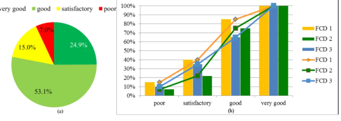
𝑛𝑛 ≥ 25 position reports during the observation hour have been examined, a total of 1,464 road segments. Fig. 1(a) shows the probabilistic qualities calculated using the quality requirements of Table 1. In order to calculate them, first mean 𝜇𝜇 and standard deviation 𝜎𝜎 were determined using the travel time measurements from FCD on the aforementioned 1,464 links in Berlins for the example hour, and then, for the links of this sample, the probabilistic qualities were estimated by determining the respective frequencies of fulfilment of the quality requirements for the four quality levels. It can be seen that, in the example hour, 78.0% of the links showed a very good or good quality of temporal coverage. For 15.0% of the links, the quality of temporal coverage was satisfactory, and for 7.0%, the quality was worse than satisfactory (“poor” quality in Fig. 1(a)). E.g. the probability of 53.1% for a very good temporal coverage expresses the estimated respective probability for an unspecified link, if at least 25 position reports have been received for this link.
Fig. 1(b) depicts the CDFs of quality measurements for three FCD fleets, discretized to the four quality levels. Fleet 2 (“FCD 2”) represents the real-world FCD from the experimental setup, whereas fleets 1 and 3 represent hypothetical data for illustration purposes. It can be seen that fleet 2 performs better than fleet 1, but cannot be compared to fleet 3 using the definition of first order stochastic dominance proposed at the end of Section 3. If more expert knowledge about the data processed from different fleets is available, higher-order SD rules may still provide a way to compare different fleets in such cases (see e.g. Levy (1992)). Further, the temporal coverage may depend on the particular time of day (e.g. on the hour of the day), since the traffic situation typically changes during a daily course. The next example in Section 5.1.2 shows how to arrive at a time series of probabilistic qualities if the assessed data are given as a times series.
5.1.2. Bluetooth
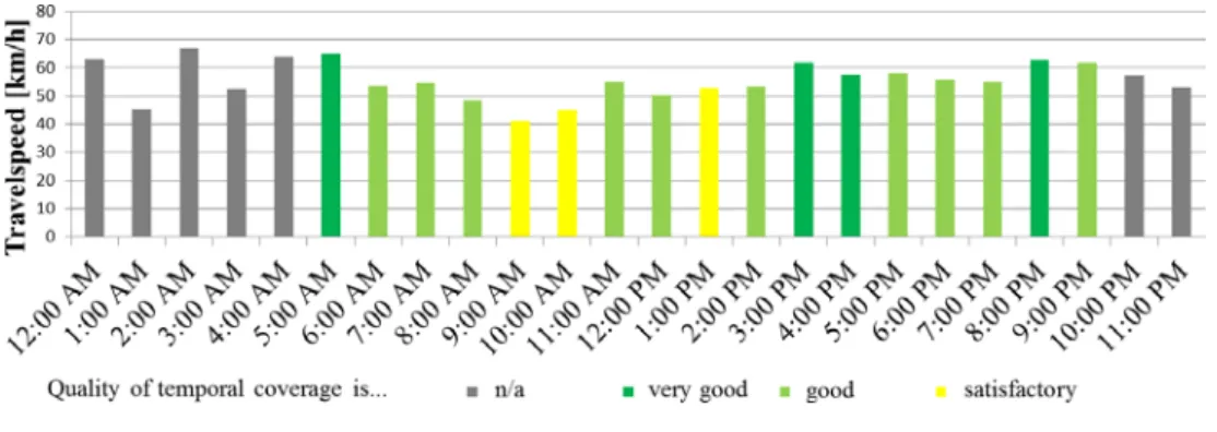
The stationary Bluetooth data assessed in the DLR-project I.MoVe have been collected from Bluetooth detectors of class 1 at the western and eastern gantry of a measuring section at Ernst-Ruska-Ufer, Berlin, Germany. The distance between the two gantries is more than 0.8 km, and the detectors have been installed at a height of approx. 8 m above the ground. This setup allows determining travel times from detections of Bluetooth devices in vehicles. More precisely, the travel times are calculated as time differences between the time stamp of a first detection at the western gantry and that of a respective match (i.e. a redetection) at the eastern gantry. Notice that several filtering steps have been applied before the calculation: e.g. multiple detections of the same device at the western gate, detections of potential multiple devices in one vehicle, and permanent detections of stationary devices have been suppressed. Moreover, impossible travel time values have been filtered out. Similar to the experiment described in Section 5.1.1, the quality of temporal coverage with pairs of matched detections, fit for the purpose of calculating a valid travel time, has been assessed. Again, the definition of quality levels in Table 1 has been used. In contrast to the previous experiment, which aimed at analyzing the spatial distribution of probabilistic quality on the different links, the focus now was to obtain a temporal distribution of the one measurement track, i.e. a diurnal course of the quality of its temporal coverage. For this purpose, the quality has been assessed repeatedly for every hour of the day, using the data of an example day (11th July, 2016). The results are given in Fig. 2, along with the measured average travel speed of the respective hour. Analogous to the previous experiment in Section 5.1.1, hours with less than 25 valid travel times have not been assessed for reasons of statistical validity. In Fig. 2, these hours (during night from 10.00 pm to 4:00 am) have been colored with grey color.
Fig. 2: Diurnal course of probabilistic qualities of temporal coverage with stationary Bluetooth detections (travel speed in km/h)
As can be seen from the results, the quality of hourly temporal coverage varies from good to very good, except for e.g. two hours during the morning rush hour, where also the travel speed shows a significant drop.
5.2. Assessment of the quality of count accuracy of induction loop detectors
This section describes the assessment of count accuracy of induction loop detectors, which are installed along the same measurement track at the Ernst-Ruska-Ufer, Berlin, Germany, already used for the experiments of Section 5.1.2. The collected data are single vehicle data which have not (yet) been aggregated for e.g. intervals of one minute. Along the measurement track, two cross section controllers have been placed successively, and in a very short distance. This has been done to facilitate a “self-evaluation” of the loop count accuracy: a deviation of the
counts observed at the two sections indicates that at least one of the controllers experienced a counting error. During the conducted experiments, detections of all types of vehicles have been counted. First, in Section 5.2.1, the assessment is done on the basis of the German TLS ( BASt (2012)). Next, in Section 5.2.2, an assessment in terms of probabilistic quality is demonstrated.
5.2.1. Assessment on the basis of the German “Technische Lieferbedingungen für Streckenstationen” (TLS) The obtained measurements have been analyzed with respect to fulfilment of the test conditions for traffic volumes as stated in the German TLS. In essence, the requirements of TLS for hourly counts are that the following conditions are respected for a period of ten hours (during daytime, and with predominantly bright daylight): 1) ∆qKfz < 3%, or rather 2) ∆qLkwÄ < 5%. Here, ∆qKfz denotes the hourly deviation of measured vehicle counts (as measured at the two successive cross sections), and ∆qLkwÄ denotes the hourly deviation of measured busses or articulated vehicles. Since all types of vehicles have been counted during the experiments, the second condition was not relevant. Notice that the test condition of TLS is actually a bit weaker than described here since it is not necessarily required that all hourly counts fulfil condition 1. More precisely, the TLS only requires that the probability distribution of “good” deviations (i.e. count differences low enough to respect condition 1) equals an analogous probability distribution of good deviations for two calibrated reference systems, with a statistical significance of (at least) 95%. Fig. 3(a) shows the percentage deviations between the vehicle counts at the two cross sections on the observation day (Tuesday, 10th May, 2015). From 8:00 am to 6:00 pm, the magnitude of the relative error stayed below the threshold of 3 percent as required by TLS (see the first condition above).
Fig. 3(a): Percentage deviations of the traffic volumes at two consecutive cross-section controllers, (b): Empirical CDF of percentage deviations of the hourly traffic volumes at two consecutive cross section controllers
As can be seen in Fig. 3(a), there are also larger deviations (at 2:00 am, 4:00 am, and 7:00 am, see the blue circle in the figure). The deviation at 4:00 am is due to a very small traffic volume, causing a meaningless numerical outlier. However, this is not the case for the measurement at 7:00 am, showing that larger deviations are possible even though the test condition of the TLS has been fulfilled. To value the importance of this observation, it is helpful to quantify how likely such larger deviations are. This is done in the next section, demonstrating how probabilistic quality can lead to a more precise assessment of data quality, and also how the use of probabilistic quality enables the comparison of sensor performances.
5.2.2. Assessment as probabilistic quality
A larger period has been chosen for the assessment of the probabilistic quality of loop count accuracy (from 1st June to 25th June, 2015). Fig. 3(b) shows the empirical CDF of the percentage deviations of the hourly traffic volumes at the two neighbored cross section controllers. In order to fulfil the quality requirement of the test procedure of the TLS, a percentage deviation of the hourly traffic volumes must be within the range of ∓3% (marked with two vertical red lines in Fig. 3(b)). In order to assess the probabilistic quality of vehicle count accuracy, the probability of fulfilment of this requirement must be quantified. Analogous to the examples in Section 3, the empirical CDF facilitates this calculation:
The probability 𝑃𝑃("absolute value of percentage error 𝑥𝑥 does not exceed 3%") can be calculated by use of the empirical CDF of the percentage deviations in the observation period via 𝑃𝑃(−3% ≤ 𝑥𝑥 ≤ 3%) = 𝐹𝐹𝑥𝑥(3%) −
𝐹𝐹𝑥𝑥(−3%) + 𝑃𝑃(𝑥𝑥 = −3%). For the complete nychthemeral data set including traffic volume counts for all 24 hours of the day, this calculation yields a probability of 𝑃𝑃nychthemeral(−3% ≤ 𝑥𝑥 ≤ 3%) ≈ 0.937 = 93.7%. If the data are restricted to contain only counts detected from 8:00 am to 6:00 pm, we obtain
𝑃𝑃8:00 am−6:00 pm(−3% ≤ 𝑥𝑥 ≤ 3%) ≈ 0.992 = 99.2%. That is, in the observation period, the probabilistic quality of nychthemeral loop count accuracy, defined as the nychthemeral (24 hours) probability of fulfilment of the quality requirement of the TLS is 93.7%. Following the test procedure of the TLS more closely, one could also focus on daily periods from 8:00 am to 6:00 pm. Then the respective probabilistic quality is significantly higher, 99.2%. Since 99.2% > 93.7%, a comparison as described at the end of Section 3 shows that the daily loop counts performed better than the nychthemeral counts.
6.Conclusion
A new probabilistic framework for data quality has been proposed, unifying and generalizing previous definitions for quality of Crosby (1979), International Organization for Standardization (1992), and Federal Highway Administration (2004). Three practical examples demonstrated the use of the proposed framework for different data sources (FCD, stationary Bluetooth sensors, and induction loop detectors). As a benefit, a more detailed picture of data quality has been given, showing how the outcomes of quality assessment (numerical probability values) are distributed over the spatial or temporal extent of the sample space. Moreover, the quality of loop count accuracy has been assessed with a higher level of detail, calculating a numerical probability of the fulfilment of requirements instead of a mere “go” or “no go” information as in the German TLS. This facilitates a subsequent use in composite quality measures, for which the proposed framework offers the well-established calculus of probability theory, using joint, marginal and conditional probabilities as well as tools for analyzing stochastic correlations and entropy measures, for instance.
7.References
BASt. "Technische Lieferbedingungen für Streckenstationen." 2012.
Brockfeld, Elmar. "Der Reiseassistent KeepMoving." 5. Tagung Mobilitätsmanagement von Morgen "Auf dem Weg zur emissionsarmen Mobilität". Berlin, 2014.
Crosby, P.B. Quality is free: the art of making quality certain. New-York: McGraw-Hill, 1979.
Davidsson, F., P. Matstoms, S. Lillienberg, and H. Andersson. OPTIS statistical analysis and PROBE simulation study. Centre for Traffic Research (CTR), 2002.
Federal Highway Administration, U.S. Department of Transportation. "Traffic Data Quality Measurement." Final Report, 2004. International Organization for Standardization. "ISO 9000: international standards for quality management." Genève, Switzerland, 1992. ITS America and U.S. Department of Transportation. "Closing the Data Gap: Guidelines for Quality Advanced Traveler Information System
(ATIS) Data." Version 1.0, 2000.
Klir, G.J. "Generalized information theory." Fuzzy Sets and Systems, 1991: 127-142.
Knapp, T.R. "Treating ordinal scales as interval scales: an attempt to resolve the controversy." Nurs Res., Mar-Apr 1990: 121-123. Levy, H. "Stochastic dominance and expected utility: survey and analysis." Management Science, Apr 1992: 555-593.
Srinivasan, K.K., and P.P. Jovanis. "Determination of Number of Probe Vehicles Required for Reliable Travel Time Measurement in Urban Network." Transportation Research Record (1537), 1996: 15 - 22.
Sullivan, G.M., and A.R. Jr. Artino. "Analyzing and interpreting data from Likert-type scales." J Grad Med Educ., Dec 2013: 541-542. Szigeti, J., P. Laborczi, and G. Gordos. "Benchmarking of Floating Car Data Sources." ITS World Congress. Stockholm, 2007. 4652-4662. Tarnoff, P.J. Getting to the INFOstructure. White Paper, TRB Roadway INFOstructure Conference, 2002.
Turner, S.M. "Defining and Measuring Traffic Data Quality: White Paper on Recommended Approaches." 83rd Annual Meeting of the Transportation Research Board. Washington. USA: National Academy of Sciences, 2004.
Turner, S.M., and D.J. Holdener. "Probe Vehicle Sample Sizes for Real-Time Information: The Houston Experience." Proc., Vehicle Navigation and Information Systems Conference. Seattle, Washington: IEEE, 1995. 3-10.